
Paper:
State Estimation of a Shape-Flexible Multifingered Robotic Hand Leveraging Multiple Proximity Sensors
Masato Morita
 , Hikaru Arita
, Kazuto Nakashima
, and Kenji Tahara
, Hikaru Arita
, Kazuto Nakashima
, and Kenji Tahara
Kyushu University
744 Motooka, Nishi-ku, Fukuoka, Fukuoka 819-0395, Japan

This paper investigates state estimation for continuum robotic fingers in feature-sparse and dynamic in-hand manipulation environments. Continuum fingers, inspired by continuum robots, offer enhanced flexibility and wider reachable workspace compared with conventional rigid-link fingers to enable grasping and manipulation tasks. However, they lack encoder-based joint angle measurements, making it difficult to determine fingertip positions, particularly under external forces during contact. This limitation hinders precision grasping and prevents the full exploitation of their high dexterity. To address this challenge, we developed a simultaneous localization and mapping framework for continuum fingers using proximity sensors. Unlike conventional simultaneous localization and mapping that assumes feature-rich environments, grasping scenarios present feature-sparse conditions with limited environmental information. We propose an estimator that fuses proximity sensing with a constant-curvature kinematic prior by replacing encoder angles with virtual joint angles. The key idea is to leverage the designed in-hand elements, namely opposing fingers and the palm, as stable reference geometry. Simulations demonstrate that the proposed estimator outperforms a kinematics-only baseline by suppressing bias and reducing position error. Three-dimensional contoured palms enhance observability, with a composite wavy palm yielding the smallest errors without temporal drift. These findings indicate that the designed in-hand geometry combined with temporal map management enables effective state estimation for continuum fingers in feature-sparse and dynamic grasping scenarios.
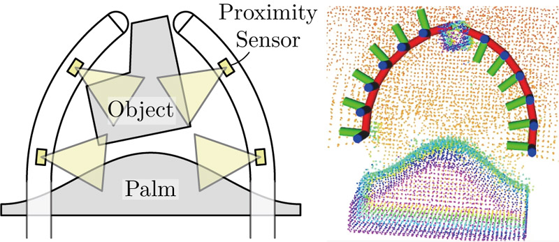
SLAM-based continuum finger estimation
1. Introduction
Accurate state estimation during physical interaction is fundamental to robotic manipulation 1. The effectiveness of in-hand manipulation depends largely on how precise the robot can perceive both its own configuration and the pose of grasped objects relative to the surrounding environment 2. However, achieving such precise state estimation is particularly challenging in confined grasping workspaces. First, conventional vision-based sensing provides limited information owing to occlusions and restricted viewing angles within the hand 2. Second, not all modern robotic hands possess high rigidity. Emerging soft robotic 3 and continuum structures, which offer advantages such as adaptability and safety, lack clearly defined joints with direct angle measurements 4,5. Third, contact forces during manipulation cause deformations that invalidate purely kinematic models 6,7. These challenges necessitate alternative sensing and estimation approaches that can operate effectively in close proximity, feature-sparse environments while accounting for structural compliance.
Proximity sensor data, as proximity information for tasks involving contact, can serve as valuable exteroceptive information 8. Unlike vision sensors whose field of view is completely obstructed when they are too close to objects, proximity sensors can obtain information at close range where physical interactions occur. Because these sensors are small and lightweight, they can be placed on the robot’s entire body to acquire environmental information surrounding the entire structure. However, existing approaches that focus on individual sensor outputs 9,10,11,12 can only measure local environmental geometry, and cannot directly estimate the robot’s overall pose with respect to the environment or grasped object. To achieve accurate state estimation for the entire robotic structure, it is necessary to integrate information from all distributed sensors and estimate the whole-body posture relative to the environment.
Simultaneous localization and mapping (SLAM) 13 has been applied to robot arms to address state uncertainty 14,15. Although studies have successfully reduced angular errors using depth or RGB-D cameras, these cameras cannot obtain information at close range and are not suitable for situations involving contacts. To address this limitation, Iwao et al. 16 proposed the integration of proximity sensors distributed over the entire body into a SLAM framework. Their method extended the discrete-time model used in SLAM to the spatial direction of the articulated structure, enabling state estimation that fuses a kinematic model based on encoder measurements with distributed time-of-flight proximity sensors. This spatial progression of estimation enables the correction of cumulative biases along the length of the structure from the root.
However, Iwao’s method 16 assumes that joint angles can be obtained from encoders at each joint, which becomes problematic for soft and continuum robotic structures that lack clearly defined joints and discrete rotation axes. For in-hand manipulation tasks, continuum robots offer significant advantages over conventional rigid-link fingers, including wider ranges of motion and better adaptability to confined spaces 17. Therefore, extending state estimation methods to continuum structures is essential to realize dexterous in-hand manipulation.
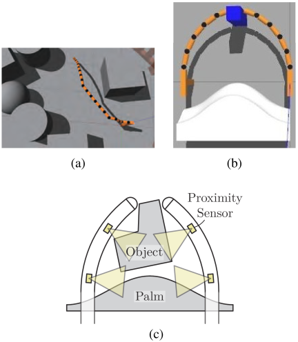
Fig. 1. (a) Environment assumed in Iwao’s method 16. (b) Environment assumed in this study. (c) Hand setup with proximity sensors on both fingers observing the object and palm.
Several limitations remain that prevent the practical application to in-hand manipulation tasks. First, unlike the feature-rich environments assumed by conventional SLAM studies 16, grasping scenarios present extremely sparse environmental features, as shown in Fig. 1(b) 18. In our previous work 19,20, we used the opposing finger and palm as in-hand landmarks within the sensors’ range, providing a stable reference geometry in sparse grasping scenarios (Fig. 1(c)). Second, grasping environments are inherently dynamic; the grasped object and opposing fingers move during manipulation, causing previously observed points to become outdated and introducing large outliers into the map. Without proper handling of these dynamic elements, both state estimation and map quality decline, preventing the reliable extraction of object geometry from accumulated point clouds. Third, the previous work only estimated a single finger’s state, but robotic hands are typically composed of multiple fingers. Accurate state estimation of all fingers is essential for successful in-hand manipulation while providing sufficient information on the grasped object’s geometry for manipulation planning.
This paper presents three key extensions to our previous work. First, we preload palm point clouds into the SLAM map to provide a stable reference geometry from the outset, improving the estimation accuracy by ensuring that persistent landmarks are available even when external features are scarce. Second, we introduce a forgetting mechanism that applies time-decay forgetting to the environmental map. By combining strong geometric constraints from the preloaded palm with temporal forgetting of outdated observations, our method maintains robust state estimation and high-quality maps even in dynamic grasping environments. This approach preserves map integrity, potentially enabling the future extraction of object geometry from accumulated point clouds for manipulation planning. Third, we extend the estimation framework to simultaneously estimate multiple fingers by running independent estimation processes for each finger and integrating their point clouds. This increases the available map information and enables better understanding of the grasped object’s geometry for manipulation planning.
The statement of our problem and corresponding proposal to solve it are as follows:
-
Problem statement
-
Continuum robotic fingers lack encoder-based joint-angle measurement capability.
-
Grasping environments provide insufficient features for conventional SLAM methods.
-
The grasping environment is dynamic, with moving objects and opposing fingers that invalidate static map assumptions.
-
-
Proposed approach
-
Substitute constant curvature model constraints for encoder measurements in SLAM.
-
Use self-body elements (palm and opposing fingers) as stable reference features, with preloaded palm point clouds to improve initial observability.
-
Introduce a forgetting mechanism to handle dynamic environments through the time-decay forgetting of outdated observations.
-
Extend simultaneous multifinger estimation by running independent processes for each finger to increase map information and enable a better understanding of the object geometry.
-
-
Key innovation
-
Enables state estimation for continuum fingers in sparse and dynamic grasping environments through designed reference structures, temporal map management, and multifinger coordination.
-
The remainder of this paper is organized as follows. Section 2 presents the estimation framework, introduces the palm shapes used as in-hand reference geometry, and explains their integration with the proximity sensor SLAM, constant-curvature virtual joint angles, forgetting mechanism, and multifinger estimation. Section 3 describes the simulation setup and evaluates the estimation accuracy with and without the palm for different palm shapes and in dynamic grasping scenarios. Section 4 discusses the effectiveness and limitations of the proposed method. Finally, Section 5 concludes the paper.
2. Method
2.1. Preliminaries on SLAM-Based State Estimation
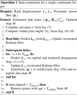
Iwao et al.’s method 16 builds upon the SLAM framework FAST-LIO2 21, originally developed for mobile robots. In the approach 16, state estimation is performed by utilizing the spatiotemporal propagation of information obtained from proximity sensors distributed across each link of the multijointed structure. The estimation process is divided into two stages: estimation of the root link and estimation of subsequent links. First, the state of the root link is estimated using standard techniques by integrating predictions from the previous time step with observations from proximity sensors mounted on the root. This procedure yields both the state of the root link and information on the surrounding environment. Once the root link has been estimated, subsequent links are estimated using a kinematic model that incorporates spatial constraints under the assumption that all links form a serial chain. In this model, the state of each link is recursively described based on the state of its adjacent upstream link. Therefore, estimation proceeds from the root toward the terminal link. This process is referred to as spatial-direction estimation. However, not all state variables propagate spatially. Variables such as joint bias, which evolve independently of inter-link constraints, are predicted from past values. Because this estimation proceeds along the time axis, it is referred to as temporal-direction estimation. This method estimates the state of each link by integrating both spatial and temporal information.
The state of the \(i\)-th link at time step \(k\) is described as follows:
The observation model derived in 21 is applied independently to each link. Using the error-state vector \(\tilde{\mathbf{x}}\), the model is linearized around the nominal state as
An error-state iterated Kalman filter 21 fused the observation data with the kinematic and observation models (Eqs. \(\eqref{eq:p}\)–\(\eqref{eq:measurement}\)) to estimate the posture of each link relative to the environment. For environmental mapping, the point-cloud data generated from the estimated states of the links were integrated into a global map. For more details, refer to 16.
2.2. Adapting SLAM Framework for Continuum Fingers
Continuum robots lack clearly defined joints and discrete rotation axes, making them infeasible to directly measure joint angles using encoders, as assumed in Iwao et al. 16. To address this limitation, we exploit the fact that the curvature of each finger is controlled by rack displacements and can be described by a constant curvature model (CCM). By discretizing the continuous structure into virtual links, the bending can be interpreted as the rotation of virtual joints. These virtual joint angles, derived from the CCM, replace encoder measurements in the SLAM framework to enable the seamless fusion of exteroceptive proximity sensing with continuum robot kinematics.
It should be noted that the CCM serves as a nominal kinematic model and not as a rigid constraint. Within the Kalman filter-based framework, the CCM-derived virtual joint angles are fused with proximity sensor observations, and the filter corrects deviations from the CCM through the bias estimation term \(b_{i,k}\) in Eq. \(\eqref{eq:b}\).
The key requirement for applying our method is the ability to estimate the curvature of the robot, which can be obtained through various method such as proprioceptive sensing or geometric models. In this study, we demonstrate the approach using the continuum finger structure proposed by Morita et al. 17.
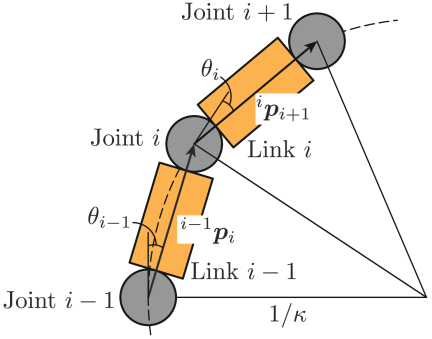
Fig. 2. Rotational angles of the virtual joints derived from the constant-curvature model.
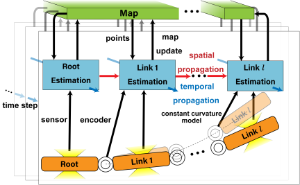
Fig. 3. Overview of the state estimation process of the proposed method when applying Iwao’s method 16 to the continuum robot fingers.
Morita et al. 17 showed that, under the constant curvature assumption, the overall curvature \(\kappa\) of the finger is related to the rack displacements \(L_1\) and \(L_2\) by
In Iwao’s formulation, the required joint angles are replaced with those obtained from the CCM. Fig. 2 yields
For the \(i\)-th joint, the rotation angle becomes
2.3. Palm Shape
This study assumes a sparse environment consisting of the state-estimation finger, opposing finger, palm, and grasped object, as shown in Fig. 1(c). Unlike the feature-rich environments assumed in conventional SLAM studies, as shown in Fig. 1(a), grasping scenarios provide limited environmental features (Fig. 1(b)) that can reduce estimation accuracy. To address this challenge, we designed the palm geometry to serve as a stable reference structure that provides persistent geometric features for proximity sensors. Fig. 4 presents the two palm shapes employed in this study: a flat palm for baseline comparison and a composite wavy palm designed to maximize geometric observability.
Figure 4(a) shows a flat palm equivalent to a rectangular solid with dimensions \(200 \times 400 \times {200}\) mm\(^3\). Fig. 4(b) shows a composite wavy palm created by removing a complex three-dimensional region(1) from the same solid.
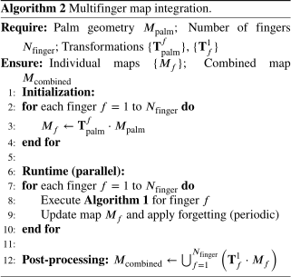
The palm geometry is represented as a prebuilt point-cloud map \(M_{\text{palm}}\) and integrated into the SLAM system as an initial map. When multiple fingers operate simultaneously, each with its own coordinate frame, the same palm point-cloud file is transformed according to each finger’s mounting configuration before integration. The specific transformation parameters and integration procedure for multifinger scenarios are detailed in Section 2.5. To avoid instability from uncertain initial pose estimates, the palm map was not immediately integrated at system startup. Instead, the integration is delayed until \(n_{\text{delay}}\) observation updates have been completed, allowing the estimator to stabilize before incorporating the prior geometric information.
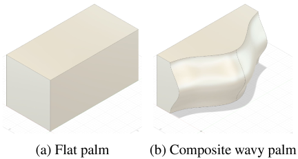
Fig. 4. Palm shapes used in the simulations.
2.4. Forgetting Mechanism
To maintain an accurate map in dynamic environments where the grasped object and opposing finger may move, we implemented the time-based forgetting mechanism that removed outdated point-cloud data. Each point \(\mathbf{q}_j\) on the map was assigned a timestamp \(t_j\) upon observation. At the current time \(t\), points that satisfy \(t - t_j > T_{\text{validity}}\) are removed from the map, where \(T_{\text{validity}}\) denotes the validity period. This forgetting mechanism prevents the accumulation of obsolete observations that no longer reflect the current environmental state. The forgetting mechanism process is executed at regular intervals \(T_{\text{interval}}\) to balance the computational load with real-time performance. These parameters were selected to accommodate typical object motion speeds while maintaining a sufficient environmental history for stable estimation.
2.5. Map Integration
In the proposed grasping scenario, multiple fingers were equipped with proximity sensors and operated simultaneously. Each finger independently performs state estimation using the method described in Section 2.2, maintaining its own environmental map through a separate estimation node and ikd-Tree structure 21. Each finger operates in its own world coordinate frame \(\mathcal{F}_{f}\), where \(f\) denotes the finger index.
At each time step, point-cloud data \(\{\mathbf{p}_j\}\) acquired by each link were transformed into the respective finger’s world frame based on the estimated link states. For the \(i\)-th link, the transformation is as follows:
To reduce computational load, the preloaded palm map was downsampled using a voxel grid filter with resolution \(v_{\text{size}} = {0.01}\) m before being transformed and integrated into each finger’s map. Each finger maintains its own ikd-Tree for efficient map management during estimation. Before insertion, each observation point was checked against existing points in the finger’s local map. If the distance to the nearest neighbor exceeds the threshold \(d_{\text{min}}\) (set equal to \(v_{\text{size}}\)), the point is added as a new map point; otherwise, the existing point is updated by incorporating the new observation. The observations acquired by each finger include not only the palm and grasped object but also other fingers, as all elements within the sensor’s detection range contribute to the environmental map.
The palm geometry, represented as an initial map, must be appropriately positioned for each finger’s coordinate frame. The same palm point cloud file was loaded for all fingers but transformed according to each finger’s mounting configuration. For the \(f\)-th finger, the palm map was transformed by \(\mathbf{T}_{\text{palm}}^{f}\), which accounts for the relative position and orientation of the finger with respect to the palm.
Although each finger independently estimates its state and maintains its own map during the operation, the resulting maps can be combined for comprehensive visualization and analysis. Let \(M_f\) denote the map generated by the \(f\)-th finger, expressed in its own coordinate frame \(\mathcal{F}_{f}\). To merge these maps, each finger’s map is transformed into a common reference frame via fixed transformations. For instance, if the first finger’s frame is chosen as the reference, the composite map is obtained by
3. Simulation
3.1. Simulation Setup
To verify the effectiveness of the proposed state estimation method in dynamic grasping scenarios, simulations were conducted in Gazebo. The simulated finger was modeled as a multijoint structure composed of five links connected in series, with each joint having a single degree of freedom about the \(z\)-axis. The origin of each link’s coordinate frame was placed at the center of its upstream joint. The \(x\)-axis is aligned with the link length, the \(y\)-axis points in the depth direction, and the \(z\)-axis points upward. Each link is \({0.04}\) m long; the joint diameter, link width, and link height are all \({0.02}\) m.
Eight proximity sensors modeled on the VL53L5CX a were evenly arranged around the circumference at the mid-length of every link. Each sensor returned 64 distance readings, yielding 512 points per link. The sensing range was set to \(0.05\)–\({1.0}\) m. The sampling rate of each sensor was set to \({15}\) Hz based on the specifications of the VL53L5CX a. To simulate calibration errors, we introduced a constant bias of 0.05 rad to the angle measurement of each joint. The distance measurement uncertainty was represented by white Gaussian noise. The three-sigma value of the noise was defined as \(\alpha r\), where \(r\) is the measured distance and \(\alpha\) is the noise-level parameter; hence the standard deviation is \(2.7\sigma = \alpha r\). The noise level was set to \(\alpha = 0.01\) for all simulations.
The grasping environment consists of two fingers positioned opposite each other with a separation distance of \({0.4}\) m. Both fingers operated simultaneously, each maintaining its own environmental map through a separate estimation node and ikd-Tree structure according to Algorithm 2. Each finger operates in its own world coordinate frame, denoted as \(\mathcal{F}_{f}\), where \(f \in \{1, 2\}\). For clarity, we refer to finger 1 as the right finger and finger 2 as the left finger. The transformation between the two fingers’ coordinate frames is \(\mathbf{T}_{2}^{1} = [\mathbf{I} \mid (0.4, 0, 0)^\top]\), which remains constant during the operation. The global coordinate frame is defined as the mounting position of the robot’s base link on the ground. The axes were set as shown in Fig. 5(a).
The composite wavy palm geometry (Fig. 4(b)) was used as the initial map \(M_{\text{palm}}\). For each finger, the palm map was transformed according to its mounting configuration: \(\mathbf{T}_{\text{palm}}^{1} = [\mathbf{I} \mid (0, 0, -0.11)^\top]\) and \(\mathbf{T}_{\text{palm}}^{2} = [\mathbf{I} \mid (0, -0.4, -0.11)^\top]\) for the right and left fingers, respectively. Key parameters were set as follows: point validity period \(T_{\text{validity}} = {5.0}\) s (unless otherwise specified), forgetting interval \(T_{\text{interval}} = {0.1}\) s, and initial map delay \(n_{\text{delay}} = 1\) round.
At each simulation trial, the right finger was driven by nominal sinusoidal joint trajectories derived from a constant-curvature prior. The ground-truth motion is produced by Gazebo physics, including contact and discretization effects, and therefore does not strictly satisfy the prior. The left finger followed a sinusoidal position command that was \(180°\) out of phase with that of the right finger. The accuracy of the proposed estimator was evaluated by comparing its output with the finger state obtained solely from the kinematic model.
Section 3.2 evaluates the effect of the forgetting mechanism on map quality and estimation accuracy in dynamic environments. Section 3.3 assesses the robustness of the proposed method when the grasped object undergoes motion during manipulation.
3.2. Effect of Forgetting Mechanism and Palm Geometry
This subsection evaluates the impact of the time-based forgetting mechanism on state estimation accuracy and map quality in dynamic grasping environments.
3.2.1. Simulation Conditions
To assess the effectiveness of the proposed method under various configurations, we systematically varied three factors: the presence of an initial map, the forgetting mechanism parameter, and palm geometry.
A rectangular object (\({0.05}~\mathrm{m} \times {0.05}~\mathrm{m} \times {0.20}~\mathrm{m}\)) was positioned at \(({0.25}~\mathrm{m}, \ {0.2}~\mathrm{m}, \ {0}~\mathrm{m})\) and remained stationary throughout the simulation, serving as a static environmental feature that both fingers can observe. Each joint of the right finger followed the command \(\theta_i = A \sin(\omega t) + B\), where \(A = {0.15}\) rad, \(\omega = {0.005}\) rad/s, and \(B = {0.15}\) rad, while the left finger followed \(\theta_i = -A \sin(\omega t) + B\). This configuration simulated a dynamic grasping scenario in which the relative positions of the fingers changed continuously.
The experimental conditions are organized as follows. Factor 1: Initial map
-
With initial map: The palm geometry is integrated as \(M_{\text{palm}}\) (Section 2.3).
-
Without initial map: No prior environmental information is provided.
Factor 2: Forgetting mechanism parameter \(\boldsymbol{T}_{\text{validity}}\)
-
\(T_{\text{validity}} = \infty\) (no forgetting mechanism): All observed points are retained indefinitely.
-
\(T_{\text{validity}} = {5.0}\) s (moderate forgetting mechanism): Points older than 5 s are removed.
-
\(T_{\text{validity}} = {1.0}\) s (aggressive forgetting mechanism): Points older than 1 s are removed.
Factor 3: Palm geometry
-
Flat palm: Planar surface (Fig. 4(a)).
-
Composite wavy palm: Three-dimensional contoured surface (Fig. 4(b)).
A full factorial design with these three factors would yield \(2 \times 3 \times 2 = 12\) conditions. For clarity, we focused on the most informative subset of conditions that demonstrated the key effects of each factor. The kinematics-only baseline was also evaluated for comparison.
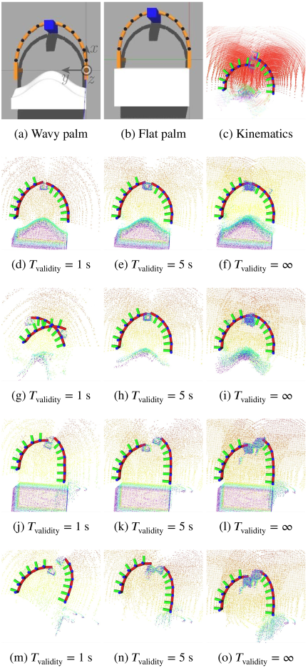
Fig. 5. Simulation snapshots. (a, b) Robot hand, (c) kinematics-only baseline, (d)–(f) composite wavy palm with initial map, (g)–(i) composite wavy palm without initial map, (j)–(l) flat palm with initial map, and (m)–(o) flat palm without initial map.
3.2.2. Results
Figure 5 shows snapshots of the simulation at \(t = {40}\) s. Figs. 5(a) and (b) show the actual robot states in the Gazebo simulation. Fig. 5(c) shows the results obtained using only the kinematic model. Figs. 5(d)–(i) show the estimated robot poses and environmental maps using the composite wavy palm. Figs. 5(j)–(o) show the results using the flat palm. All subfigures are shown from the same viewpoint.
Although the commanded motion is left–right symmetric, the kinematics-only baseline (Fig. 5(c)) produces an asymmetric estimate because the simulated joint angle measurements include a bias of \(+{0.05}\) rad applied uniformly to all joints on both fingers. Owing to the coordinate frame definitions, this uniform bias resulted in the left finger appearing more deeply curved, while the right finger appeared less curved. Consequently, the kinematics-only results exhibited large estimation errors.
For the composite wavy palm with the initial map (Figs. 5(d)–(f)), the estimated robot poses generally agreed with the ground truth shown in Fig. 5(a). The environmental maps became clearer as \(T_{\text{validity}}\) decreased. However, with \(T_{\text{validity}} = {1}\) s (Fig. 5(d)), parts of the grasped object geometry are lost because of the forgetting mechanism. With \(T_{\text{validity}} = \infty\) (Fig. 5(f)), incorrect map reconstructions caused by early inaccurate pose estimates were visible. With \(T_{\text{validity}} = {1}\) s and \({5}\) s (Figs. 5(d) and (e)), these erroneous maps were removed by the forgetting mechanism, resulting in accurate object shape reconstruction.
For the composite wavy palm without an initial map (Figs. 5(g)–(i)), the estimated robot poses generally agreed with the ground truth except for \(T_{\text{validity}} = {1}\) s (Fig. 5(g)), where significant pose deviation occurs. With \(T_{\text{validity}} = {5}\) s (Fig. 5(h)), the environmental map is relatively clear.
For the flat palm (Figs. 5(j)–(o)), both the estimated robot poses and environmental maps were less accurate compared to the composite wavy palm conditions. The snapshot of \(T_{\text{validity}} = {1}\) s with the initial map is omitted as it yields results similar to those of \(T_{\text{validity}} = {5}\) s.
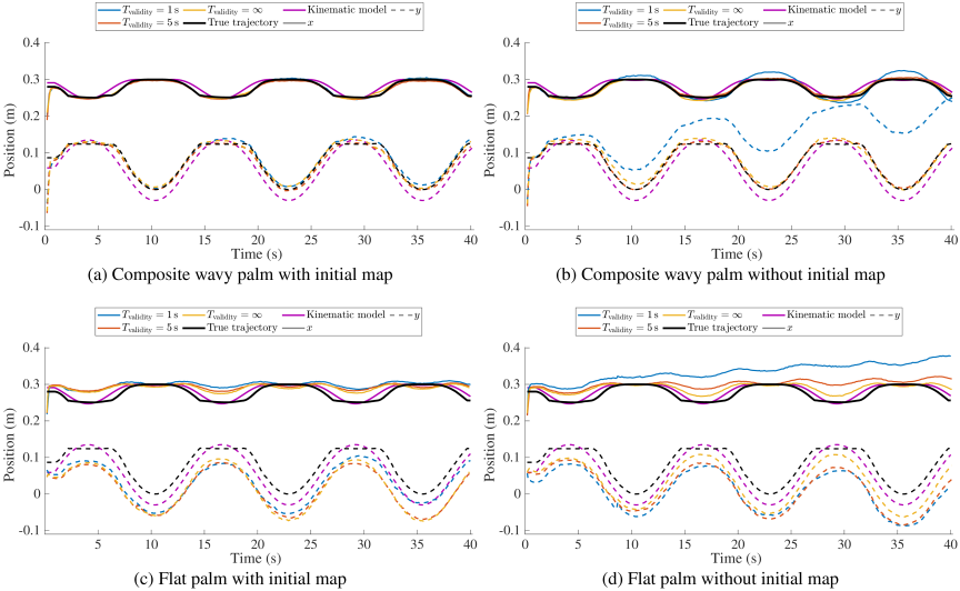
Fig. 6. Comparison of tip-link origin trajectories of the right finger estimated by the proposed method (colored lines), kinematics only (purple line), and ground truth (black line) under different palm and initial map conditions.
Figure 6 shows the trajectories of the tip-link origin. In these figures, the solid and dashed lines represent the \(x\)- and \(y\)-components, respectively. Different colors indicate different values of \(T_{\text{validity}}\) as well as the kinematics-only baseline and ground truth. Table 1 lists the root mean square error (RMSE) of the tip-link origin in \(x\), \(y\), \(z\), and their Euclidean combination for each condition. The kinematics-only baseline, which relies solely on the CCM without SLAM-based estimation, was common across all conditions and yielded a total RMSE of \({0.026}\) m with \(x = {0.008}\) m, \(y = {0.024}\) m, and \(z = {0.000}\) m.
Table 1. Estimated RMSE in meters for the right finger tip-link.
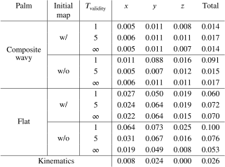
Comparing conditions without the forgetting mechanism (\(T_{\text{validity}} = \infty\)) and initial map, the composite wavy palm achieved lower errors in the \(x\)- and \(y\)-directions (\(x = {0.006}\) m, \(y = {0.011}\) m) than the flat palm (\(x = {0.019}\) m, \(y = {0.049}\) m). With the forgetting mechanism (\(T_{\text{validity}} = {5}\) s) and initial map enabled, the composite wavy palm maintained errors in the \(x\)- and \(y\)-directions at \({0.006}\) m and \({0.011}\) m, respectively. In contrast, the flat palm with the initial map and \(T_{\text{validity}} = {5}\) s exhibited larger errors (\(x = {0.024}\) m, \(y = {0.064}\) m) compared with the case without the initial map (\(x = {0.031}\) m, \(y = {0.067}\) m).
Regardless of the palm geometry, enabling the initial map generally reduced estimation errors. For the composite wavy palm with \(T_{\text{validity}} = {5}\) s, the total RMSE increased slightly from \({0.015}\) m without the initial map to \({0.017}\) m with the initial map. For the flat palm with \(T_{\text{validity}} = {5}\) s, the total RMSE decreased from \({0.076}\) m without the initial map to \({0.072}\) m with the initial map.
With a short validity period (\(T_{\text{validity}} = {1}\) s) and without an initial map, the composite wavy palm exhibited significantly larger errors in the \(x\)- and \(y\)-directions (\(x = {0.011}\) m, \(y = {0.088}\) m, total RMSE \(= {0.091}\) m) because the forgetting mechanism became overly aggressive. In contrast, when the initial map was present, the same configuration achieved \(x = {0.005}\) m, \(y = {0.011}\) m, and total RMSE \(= {0.014}\) m. For the flat palm, \(T_{\text{validity}} = {1}\) s without the initial map results in the largest errors across all conditions (\(x = {0.064}\) m, \(y = {0.073}\) m, total RMSE = \({0.100}\) m).
Among all conditions, the composite wavy palm with the initial map and \(T_{\text{validity}} = {1}\) s (aggressive forgetting mechanism) achieved the smallest total RMSE at \({0.014}\) m. The kinematics-only baseline (\({0.026}\) m) is smaller than most flat palm configurations, but larger than most composite wavy palm configurations.
3.3. State Estimation with Moving Object
This subsection assesses the robustness of the proposed method when the grasped object undergoes motion during manipulation, extending the evaluation beyond the static object scenario in Section 3.2.
3.3.1. Simulation Conditions
To evaluate the proposed method in realistic manipulation scenarios, we designed an automated grasping sequence that systematically tested the estimator’s ability to track both the robot and object motions while maintaining map consistency. A rectangular object (\({0.05}~\mathrm{m} \times {0.05}~\mathrm{m} \times {0.20}~\mathrm{m}\)) was initially positioned at \(({0.5}~\mathrm{m}, \ {0.2}~\mathrm{m}, \ {0.1}~\mathrm{m})\). The sequence consisted of the following five phases:
Phase A: Initialization. Both robot arms are reset to an initial configuration with joint angles of 0.15 rad and a 1.0 s settling period.
Phase B: Preliminary robot motion. Both fingers execute one complete cycle of sinusoidal joint motion as defined in Section 3.2.1, with a cycle duration of approximately 12.6 s.
Phase C: Object approach. The object moves diagonally from \(({0.5}~\mathrm{m}, \ {0.25}~\mathrm{m}, \ {0.1}~\mathrm{m})\) (Fig. 7(a)) to \(({0.15}~\mathrm{m}, \ {0.15}~\mathrm{m}, \ {0.1}~\mathrm{m})\) over 5.0 s (Fig. 7(b)), and then retracts to \(({0.25}~\mathrm{m}, \ {0.2}~\mathrm{m}, \ {0.1}~\mathrm{m})\) over 2.0 s (Fig. 7(c)). This diagonal trajectory intentionally creates residual points of the dynamic object that spatially overlap with the final object position, enabling the evaluation of the forgetting mechanism’s ability to handle temporally inconsistent map data.
Phase D: Post-approach robot motion. Following Phase C, both robot arms execute sinusoidal joint motion in the reverse direction, as defined in Section 3.2.1.
Phase E: Object rotation. After one complete cycle of Phase D, the object is instantaneously rotated in place by \(+20°\) about the \(z\)-axis (Fig. 7(d)), while both robot arms continue the sinusoidal motion for one additional cycle. This instantaneous orientation change introduces spatially overlapping but geometrically inconsistent observations at the final object position, directly testing whether the forgetting mechanism can eliminate outdated map data that conflicts with current sensor readings.
Throughout all phases, the composite wavy palm (Fig. 4(b)) served as a static reference geometry and was integrated as the initial map \(M_{\text{palm}}\) in all conditions to provide stable features. The forgetting mechanism parameter \(T_{\text{validity}}\) and kinematics-only baseline conditions were the same as those in Section 3.2.1.
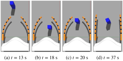
Fig. 7. Object positions during key phases. (a) Initial object position at \(({0.5}~\mathrm{m}, \ {0.25}~\mathrm{m}, \ {0.1}~\mathrm{m})\) (before Phase C). (b) Object near the closest approach position at \(({0.15}~\mathrm{m}, \ {0.15}~\mathrm{m}, \ {0.1}~\mathrm{m})\) during Phase C. (c) Object at the retracted position \(({0.25}~\mathrm{m}, \ {0.2}~\mathrm{m}, \ {0.1}~\mathrm{m})\) (end of Phase C). (d) Object after instantaneous \(+20°\) rotation about the \(z\)-axis (Phase E).
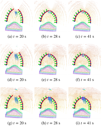
Fig. 8. Simulation snapshots under different forgetting mechanism settings at three time points. \(t = {20}\) s corresponds to the end of Phase C, \(t = {28}\) s shows the state during Phase D before object rotation, and \(t = {41}\) s represents the final state after Phase E. Rows show results for (a)–(c) \(T_{\text{validity}} = {1.0}\) s, (d)–(f) \(T_{\text{validity}} = {5.0}\) s, and (g)–(i) \(T_{\text{validity}} = \infty\).
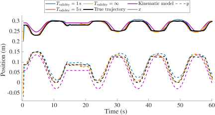
Fig. 9. Comparison of tip-link origin trajectories of the right finger estimated by the proposed method under different forgetting mechanism settings (colored lines), kinematics-only baseline (purple line), and ground truth (black line) in the moving object scenario.
3.3.2. Results
Figure 8 presents the simulation snapshots at three key time points: \(t = {20}\) s at the end of Phase C, \(t = {28}\) s during Phase D before the object rotation in Phase E, and \(t = {41}\) s after Phase E completion. Fig. 9 shows the trajectories of the tip-link origin estimated by the proposed method under different forgetting mechanism settings, compared with the kinematics-only baseline and ground truth.
When the forgetting mechanism is enabled (Figs. 8(a)–(f)), the observations acquired during the object motion in Phase C are progressively removed from the map. At \(t = {28}\) s (Figs. 8(b) and (e)), the object shape reconstruction was less complete compared to the condition without the forgetting mechanism (Fig. 8(h)) because residual points from the diagonal approach trajectory were discarded. However, after the instantaneous rotation in Phase E, the forgetting mechanism settings (Figs. 8(c) and (f)) show cleaner maps that retained only the current object geometry, while the no-forgetting mechanism condition (Fig. 8(i)) accumulated both pre- and post-rotation observations, creating spatially overlapping but geometrically inconsistent point clouds at the object location.
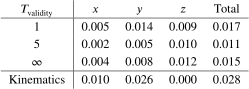
Table 2 shows that the proposed method achieves higher estimation accuracy than the kinematics-only baseline across all forgetting mechanism settings. Notably, the moderate forgetting mechanism setting (\(T_{\text{validity}} = {5.0}\) s) yielded the lowest overall RMSE of 0.011 m, outperforming both the no-forgetting mechanism condition (0.015 m) and aggressive setting (0.017 m). This result indicates that an appropriately tuned forgetting mechanism parameter can balance two competing factors: retaining sufficient environmental structure for pose estimation while eliminating outdated observations that conflict with current sensor readings.
As shown in Fig. 9, the condition without the forgetting mechanism (\(T_{\text{validity}} = \infty\)) exhibited larger trajectory deviations during Phases C and D when residual points from the object’s diagonal approach path remained in the map and spatially overlapped with the object’s final position. These residual points created ambiguous geometric constraints that temporarily degraded pose estimation accuracy. In contrast, the moderate forgetting mechanism setting (\(T_{\text{validity}} = {5.0}\) s) maintained more consistent trajectory accuracy throughout the sequence by removing stale observations before they accumulated into significant conflicts. The aggressive setting (\(T_{\text{validity}} = {1.0}\) s) shows comparable performance to the moderate configuration in this scenario, with slightly higher errors in the \(y\)- and \(z\)-components, suggesting that the 1.0 s retention time approached the lower bound to maintain sufficient environmental information during the dynamic phases.
Table 2. Estimated RMSE in meters for the right finger tip-link under moving object condition.
4. Discussion
This section discusses why the proposed estimation framework stabilizes the estimation in sparse environments, its current limitations, and promising directions for future research.
4.1. Key Factors for Robust Estimation
The primary reason that three-dimensional palm geometries outperform a flat plane is that the measurement model in Eq. \(\eqref{eq:measurement}\) assumes a local planar fit. Therefore, the geometric constraints strengthen as the curvature and depth cues increase. A flat palm induces left-right symmetry in the environment, making corridor-like ambiguities likely. In particular, the composite wavy palm continuously supplies depth and curvature cues, simultaneously improving map quality and pose observability.
Both the forgetting mechanism and the introduction of an initial map are necessary for robust estimation. The forgetting mechanism is effective in dynamic environments and suppresses the influence of erroneous observations. The initial map is effective because the relative positions of the robot’s fingers and palm are known, providing a stable reference geometry. With the forgetting mechanism alone, the map may be significantly lost depending on the robot’s pose. Although the palm provides information, incorrect pose estimation can prevent accurate map construction. In extreme cases, as shown in Fig. 5(g), the system strongly trusts the CCM owing to sparse environmental information, causing the robot base frame to rotate. By having a stable reference geometry such as the initial map, pose estimation and map construction become stable.
The validity period of the points in the forgetting mechanism must be appropriately set. In this study, it was determined empirically to match the robot’s periodic motion. An extreme case, in which an overly short validity period causes estimation failure, is shown in Fig. 5(g). Ideally, dynamic adjustment of the validity period based on observation density and distribution would be desirable, which represents a limitation of the current approach.
Penetration of the grasped object occurs because the line of sight is occluded near the object, observations become scarce, and the filter is pulled toward the CCM. In our experiments with the composite wavy palm, the error did not increase over time and remained within a range that did not hinder task-level performance.
Because the proposed method is based on a Kalman filter, the degree of trust placed in the CCM is governed by the process noise covariance matrix \(\mathbf{Q}\) of \(\boldsymbol{\omega}_i\) in Eq. \(\eqref{eq:state_link}\), which served as the design hyperparameter. In the encoder-based setting of Iwao et al. 16, the encoder readings were relatively accurate; therefore, \(\mathbf{Q}\) was set to be small. For continuum robots, however, the CCM is a less reliable nominal model whose primary role is to provide a kinematic reference that prevents the estimator from diverging when the sensor observations are sparse. Accordingly, \(\mathbf{Q}\) should be set to be larger to reflect this lower confidence level. Furthermore, the appropriate covariance may depend on the finger’s geometric configuration; for example, a short finger segment is better approximated by a constant curvature than a long one, suggesting that dynamically adjusting \(\mathbf{Q}\) based on the finger length or curvature can improve the estimation robustness.
4.2. Understanding the Forgetting Mechanism
The simulation design in Section 3.3 deliberately introduces two sources of spatially overlapping but temporally inconsistent observations. First, the diagonal object trajectory in Phase C leaves residual points that spatially overlap with the object’s final position, unlike a purely linear approach-retract motion, where residual points would be spatially separated. Second, the instantaneous rotation in Phase E creates geometrically inconsistent point clouds at the same location. These design choices successfully demonstrated the effectiveness of the forgetting mechanism in realistic manipulation scenarios, where object motion created ambiguous environmental data, as evidenced by the superior performance of the moderate setting (\(T_{\text{validity}} = {5.0}\) s) over disabling the forgetting mechanism in Table 2.
The necessity of the forgetting mechanism depends critically on the spatial relationship between residual points and the current object location. When residual points are spatially separated from the current object position, they do not directly interfere with the measurement model in Eq. \(\eqref{eq:measurement}\) during subsequent estimation steps. In such cases, the forgetting mechanism provides limited benefit because the residual points lie outside the local neighborhood considered by the local planar fit assumption, and thus do not attract the point cloud alignment toward incorrect geometries.
In contrast, when residual points spatially overlap with or lie in close proximity to the current object position, the measurement model attempts to fit current sensor readings to both the correct current and the incorrect residual geometries. This ambiguity reduces the alignment accuracy and introduces bias in the pose estimation. The forgetting mechanism addresses this issue by removing outdated observations before they accumulate into spatially overlapping conflicts.
The results in Section 3.3 confirm this principle. The diagonal trajectory in Phase C and instantaneous rotation in Phase E create scenarios in which the residual and current observations spatially overlap, leading to the observed performance advantage of a moderate forgetting mechanism setting over disabling the forgetting mechanism. This demonstrates that the forgetting mechanism is particularly valuable in manipulation tasks involving complex object motion within confined workspaces, where the likelihood of spatial overlap between past and present observations is high.
4.3. Extension to Multifinger Systems
This study focused on pose estimation for a single finger, with the opposing finger serving as part of the reference geometry. While both fingers independently maintained their own maps in the current implementation, extending this to a multifinger configuration with shared environmental maps and interfinger constraints represents a promising direction. However, careful consideration is required when sharing maps between fingers because geometric ambiguities may arise. For instance, when both fingers observe the planar surfaces of a rectangular object, the right and left faces may be erroneously identified as the same plane, potentially propagating errors between fingers. Maintaining independent maps for each finger avoids such error propagation while still leveraging the palm and opposing finger as reference geometry.
4.4. Future Directions
Several promising directions have emerged from this study. First, incorporating the extension and contraction states into the kinematic model would enable more accurate state estimation for continuum fingers with variable lengths. The current CCM assumes constant finger length. However, the proposed finger structure 17 supports both extension and bending, which can provide additional degrees of freedom for manipulation tasks.
Second, extracting the object geometry from the accumulated point clouds represents an important next step toward autonomous manipulation planning. While the current work focuses on state estimation, the high-quality environmental maps generated by our method, particularly with the composite wavy palm and moderate forgetting mechanism setting, contain sufficient geometric information about grasped objects. Developing methods to segment and reconstruct object shapes from these maps would enable the robot to reason about object properties and plan manipulation strategies accordingly.
Third, co-design of the palm geometry, sensor placement, and estimation parameters offers the potential for further performance improvements. The composite wavy palm was designed heuristically to maximize geometric observability, but systematic optimization of these design parameters could yield even better results.
5. Conclusions
This study addressed state estimation for shape-flexible multifingered hands performing in-hand manipulation in feature-sparse and dynamic environments. To overcome the limitations of vision-based sensing and encoder-dependent kinematics in confined grasping workspaces, we formulated a SLAM-based estimator that fuses constant-curvature kinematic priors with distributed proximity sensing for continuum fingers. The proposed method exploits user-designable in-hand structures, namely, the palm and opposing fingers, as persistent geometric landmarks to enable observability even when external environmental features are scarce. To cope with the motion of grasped objects and fingers, we further introduced a forgetting mechanism with time-decay forgetting and an initial palm point cloud, which together maintained a consistent environmental map during the dynamic interaction.
Simulation results showed that the proposed estimator suppressed bias and reduced fingertip position error compared with a kinematics-only baseline. The combination of the forgetting mechanism and palm preloading was crucial for robust estimation in dynamic grasping scenarios, preventing map corruption while preserving stable reference geometry. Three-dimensional palm geometries enhanced the pose observability and map quality, and the composite wavy palm achieved the smallest errors without temporal drift. The resulting environmental maps contained sufficient geometric information about grasped objects, suggesting the feasibility of subsequent object-shape estimation and manipulation planning.
Acknowledgments
This work was partially supported by JSPS KAKENHI Grant Number JP24H00726 and the Kyushu University Foundation.
Footnotes
(1) First, the region bounded by \(y = 20\cos\bigl(\tfrac{2\pi}{200}z\bigr)-30\) for \(-100 < z < 100\) and by \(y = 100,\;z = \pm 100\) is projected onto the plane \(x = 100\). Next, this projected region is swept along the path \(y = 50\cos\bigl(\tfrac{2\pi}{400}x\bigr)+50\) for \(-200 < x < 200\) and removed.
- [1] M. Suomalainen, Y. Karayiannidis, and V. Kyrki, “A survey of robot manipulation in contact,” Robot. Auton. Syst., Vol.156, Article No.104224, 2022. https://doi.org/10.1016/j.robot.2022.104224
- [2] S. Suresh, H. Qi, T. Wu, T. Fan, L. Pineda, M. Lambeta, J. Malik, M. Kalakrishnan, R. Calandra, M. Kaess, J. Ortiz, and M. Mukadam, “NeuralFeels with neural fields: Visuotactile perception for in-hand manipulation,” Sci. Robot., Vol.9, No.96, Article No.eadl0628, 2024. https://doi.org/10.1126/scirobotics.adl0628
- [3] W. Zhao, Y. Zhang, and N. Wang, “Soft Robotics: Research, Challenges, and Prospects,” J. Robot. Mechatron., Vol.33, No.1, pp. 45-68, 2021. https://doi.org/10.20965/jrm.2021.p0045
- [4] D. Rus and M. T. Tolley, “Design, fabrication and control of soft robots,” Nature, Vol.521, No.7553, pp. 467-475, 2015. https://doi.org/10.1038/nature14543
- [5] J. Burgner-Kahrs, D. C. Rucker, and H. Choset, “Continuum Robots for Medical Applications: A Survey,” IEEE Trans. Robot., Vol.31, No.6, pp. 1261-1280, 2015. https://doi.org/10.1109/tro.2015.2489500
- [6] J. M. Ferguson, D. C. Rucker, and R. J. Webster, “Unified Shape and External Load State Estimation for Continuum Robots,” IEEE Trans. Robot., Vol.40, pp. 1813-1827, 2024. https://doi.org/10.1109/tro.2024.3360950
- [7] Z. Wang, G. Wang, X. Chen, and N. M. Freris, “Kinematic Modeling and Control of a Soft Robotic Arm with Non-constant Curvature Deformation,” Proc. IEEE Int. Conf. Robot. Autom. (ICRA), pp. 12749-12755, 2024. https://doi.org/10.1109/icra57147.2024.10611049
- [8] S. E. Navarro, S. Muhlbacher-Karrer, H. Alagi, H. Zangl, K. Koyama, B. Hein, C. Duriez, and J. R. Smith, “Proximity Perception in Human-Centered Robotics: A Survey on Sensing Systems and Applications,” IEEE Trans. Robot., Vol.38, No.3, pp. 1599-1620, 2022. https://doi.org/10.1109/tro.2021.3111786
- [9] H. Arita, “A fast optical proximity sensor skin that contains an analog computing circuit and can cover an entire link,” Adv. Robot., Vol.37, No.17, pp. 1083-1099, 2023. https://doi.org/10.1080/01691864.2023.2239320
- [10] S. J. Moon, J. Kim, H. Yim, Y. Kim, and H. R. Choi, “Real-Time Obstacle Avoidance Using Dual-Type Proximity Sensor for Safe Human-Robot Interaction,” IEEE Robot. Autom. Lett., Vol.6, No.4, pp. 8021-8028, 2021. https://doi.org/10.1109/lra.2021.3102318
- [11] Y. Ding, F. Wilhelm, L. Faulhammer, and U. Thomas, “With Proximity Servoing towards Safe Human-Robot-Interaction,” Proc. IEEE/RSJ Int. Conf. Intell. Robots Syst. (IROS), pp. 4907-4912, 2019. https://doi.org/10.1109/iros40897.2019.8968438
- [12] S. Suyama, M. Nakajima, H. Arita, and M. Tanaka, “Control of a Snake Robot With Proximity Sensors to Adapt for Two Variable Planes,” IEEE Access, Vol.12, pp. 46864-46880, 2024. https://doi.org/10.1109/access.2024.3382205
- [13] X. Yue, Y. Zhang, J. Chen, J. Chen, X. Zhou, and M. He, “LiDAR-based SLAM for robotic mapping: state of the art and new frontiers,” Ind. Robot., Vol.51, No.2, pp. 196-205, 2024. https://doi.org/10.1108/ir-09-2023-0225
- [14] M. Klingensmith, S. S. Sirinivasa, and M. Kaess, “Articulated Robot Motion for Simultaneous Localization and Mapping (ARM-SLAM),” IEEE Robot. Autom. Lett., Vol.1, No.2, pp. 1156-1163, 2016. https://doi.org/10.1109/lra.2016.2518242
- [15] C. Sorensen, P. Hyatt, M. Ricks, S. Nielsen, and M. D. Killpack, “Soft Robot Configuration Estimation and Control Using Simultaneous Localization and Mapping,” Proc. IEEE/RSJ Int. Conf. Intell. Robots Syst. (IROS), pp. 616-623, 2021. https://doi.org/10.1109/iros51168.2021.9635896
- [16] K. Iwao, H. Arita, and K. Tahara, “State Estimation and Environment Recognition for Articulated Structures via Proximity Sensors Distributed over the Whole Body,” IEEE Robot. Autom. Lett., Vol.10, No.3, pp. 3030-3037, 2025. https://doi.org/10.1109/lra.2025.3539117
- [17] M. Morita, H. Arita, A. Kanada, and K. Tahara, “Multi-fingered Robotic Hand with Shape Flexibility for Expanding the Feasible Range of In-hand Manipulation,” Proc. IEEE/SICE Int. Symp. Syst. Integr. (SII), pp. 216-221, 2025. https://doi.org/10.1109/SII59315.2025.10870904
- [18] M. Morita, K. Iwao, H. Arita, and K. Tahara, “State Estimation of a Shape-flexible Multi-fingered Hand Using Multiple ToF Sensors,” Proc. SICE Syst. Integr. Div. Annu. Conf. (SI2024), pp. 1399-1400, 2024 (in Japanese).
- [19] M. Morita, H. Arita, K. Nakashima, and K. Tahara, “State Estimation of a Shape-flexible Multi-fingered Robotic Hand Leveraging Multiple Proximity Sensors Measuring an Ambient Environment including the Self-body and a Constant Curvature Model,” Proc. IEEE/SICE Int. Symp. Syst. Integr. (SII), 2026. https://doi.org/10.1109/SII64115.2026.11404608
- [20] M. Morita, K. Iwao, H. Arita, K. Nakashima, and K. Tahara, “State Estimation of a Shape-flexible Multi-fingered Robotic Hand Using Multiple Proximity Sensors Measuring an Ambient Environment including the Self-body,” Proc. JSME Robot. Mechatron. Conf. (Robomec), 1P1-L03, 2025 (in Japanese).
- [21] W. Xu, Y. Cai, D. He, J. Lin, and F. Zhang, “FAST-LIO2: Fast Direct LiDAR-Inertial Odometry,” IEEE Trans. Robot., Vol.38, No.4, pp. 2053-2073, 2022. https://doi.org/10.1109/tro.2022.3141876
- [a] STMicroelectronics, “Time-of-flight (tof) 8x8 multizone ranging sensor with wide field of view.” https://www.st.com/en/imaging-and-photonics-solutions/vl53l5cx.html [Accessed November 20, 2025].
This article is published under a Creative Commons Attribution-NoDerivatives 4.0 Internationa License.