
Paper:
Quantitative Evaluation of Postural Recovery During Human Walking by System Identification
Yasushi Hiroyama*, Hiroto Mori*, Ayato Kanada**
 , Yasutaka Nakashima***
, and Motoji Yamamoto***
, Yasutaka Nakashima***
, and Motoji Yamamoto***
*Department of Mechanical Engineering, Graduate School of Engineering, Kyushu University
744 Motooka, Nishi-ku, Fukuoka, Fukuoka 819-0395, Japan
**Department of Mechanical and Intelligent Systems Engineering, The University of Electro-Communications
1-5-1 Chofugaoka, Chofu, Tokyo 182-8585, Japan
***Faculty of Engineering, Kyushu University
744 Motooka, Nishi-ku, Fukuoka, Fukuoka 819-0395, Japan

This paper proposes a method to quantitatively evaluate human posture recovery performance when mechanical disturbances are applied during walking, considering that human falls mainly occur while walking. During walking, the reaction force from the soles of the feet acts as a disturbance during normal walking, which makes it difficult to distinguish between postural responses due to intentional mechanical disturbances and those due to normal walking. Furthermore, it is not easy to reproducibly apply mechanical disturbances during walking. The study uses a treadmill with independent left and right belts. The speed difference between the left and right belts is used as the disturbance input, and the dynamics of human postural correction due to disturbances is identified using system identification with the response of the center of pressure as the output. A method to quantitatively evaluate the posture recovery ability is proposed using the pole distribution of the identified dynamics model. The effectiveness of the proposed method is shown by experimentally demonstrating that there is a quantitatively significant difference in posture recovery performance when posture recovery ability is artificially reduced compared to when it is not reduced.
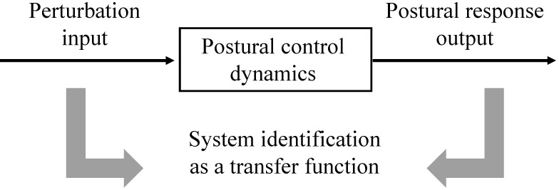
Input and output in system identification
1. Introduction
1.1. Fall Risk Assessment
According to the World Health Organization, falls are the second most common cause of unintentional injury and death worldwide, after traffic accidents, killing approximately 684,000 people annually a. Falls are a major problem for society because they lead to a decline in activities of living and increase medical costs 1. It has been reported that falls often occur when mechanical or kinematic disturbances are applied to a person, such as slipping or tripping 2,3,4.
To evaluate the fall risk, the Get Up and Go test 5 and the time required to complete it, the Timed Up and Go test 6 are used as simple fall risk assessment indicators. Other commonly used instruments include the Berg baklance scale 7, which measures balance maintenance ability, and the Performance-Oriented Mobility Assessment 8, which comprehensively evaluates gait quality and balance. Furthermore, MoS, defined as the distance between the extrapolated center of gravity \(X_{\mathrm{CoM}}\), which is the future position of the center of gravity taking into account velocity \(V_{\mathrm{CoM}}\), and the boundary of the base of support (BoS), is used as a measure of postural stability margin 9,10,11,12,13. However, MoS, for example, indicates the stable limit distance at which a fall does not occur during a specific gait cycle, and does not represent the inherent postural stabilization performance of that individual.
Since falls are common during walking, the ability to return to normal walking posture when it is disrupted by various external disturbances during walking is thought to be important in assessing the risk of falls. Therefore, when assessing the risk of tipping over when an external disturbance is applied, it is important not only to look at the resulting stability margin, but also to evaluate the postural control dynamics, which shows how the postural control system responds. Furthermore, Miyazaki et al. 14 are discussing strategies to improve posture control ability itself.
1.2. Quantifying Postural Recovery Ability
Previous research by Togoe et al. has shown a fall risk assessment method that focuses on postural control dynamics 15. They apply an impact force to the lower limbs from a standing position and obtain postural change output by measuring the center of pressure (COP). Using these input/output response results, the posture control dynamics is experimentally obtained as a transfer function through system identification. By evaluating the poles of this transfer function, they quantitatively assess the ability to recover posture from an upright position.
This method makes it possible to quantitatively evaluate postural control ability during static standing. However, since most falls occur while walking 3,4, it is important to evaluate postural control ability while walking. During walking, center of gravity sway occurs, depending on walking period and walking speed. This is equivalent to being constantly affected by mechanical disturbances during stationary standing, making it difficult to evaluate postural recovery ability.
This paper extends the previous method for assessing the risk of falling during stationary standing to the case of walking in order to evaluate the risk of falling while normal walking. There are two challenges for this problem. The first one is that it is difficult to distinguish between COP fluctuations due to normal walking and those due to postural control in response to disturbances, making identification using only the latter difficult.
The second problem is that it is not so easy to apply disturbances that excite the postural control dynamics during walking. Several studies have investigated the effects and variability of walking motion by applying some kind of disturbance during walking. However, few of these studies have focused on postural control dynamics, and it is unclear what kind of disturbances excite postural control dynamics.
Regarding the first point, this paper proposes a method for identifying the postural recovery dynamics system by using the results of time-frequency analysis to remove, to some extent, the COP fluctuation component caused by normal walking. In a time-frequency analysis of COP fluctuations that include elements of normal walking, we show that frequency characteristics are observed immediately after the application of a disturbance. This suggests that it is possible to identify postural control dynamics even without completely eliminating COP fluctuations during normal walking.
To address the second issue, we use a split treadmill and suddenly reduce the speed of only one of the belts. Using the techniques, we propose a method to derive a mathematical model of postural control dynamics, which represents the postural response to disturbances during walking, using a system identification method. We then propose a method to quantitatively evaluate postural stabilization performance during walking based on the pole placement of the mathematical model.
2. Postural Recovery System Identification
This section describes a method for identifying the postural recovery dynamics when mechanical disturbances are applied during walking. First, the inputs and outputs to be used for system identification are selected. Then a method for extracting the period of input/output data obtained in an experiment that expresses attitude control dynamics is proposed. Finally, we describe a system identification method (Fig. 1).
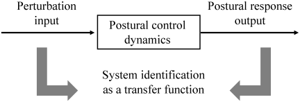
Fig. 1. Input and output in system identification.
2.1. Postural Response System Output
Physical quantities that represent human postural responses during walking include the center of mass (CoM), the future position of the center of gravity (\(X_{\mathrm{CoM}}\)) 12, walking speed 16, the acceleration of the head and trunk 17, and the variance of step length and step width 18. The CoM, \(X_{\mathrm{CoM}}\), walking speed, and head and trunk acceleration are control targets in postural control and appear as results of postural control.
On the other hand, the COP 19 is something that humans actively change during postural control. Because this includes the influence of acceleration, it is thought to be an index that more directly reflects human postural control, taking dynamics into account (Fig. 2). Furthermore, unlike stride length and step width, COP can be obtained as a continuous value, making it suitable for system identification. Therefore, in this paper, we measure COP as a postural response to external disturbances.
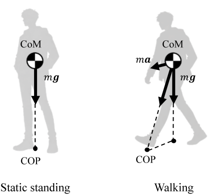
Fig. 2. Conceptual relationship between CoM and COP.
2.2. Postural Response System Input
To date, various disturbance methods have been used to obtain postural responses during walking. For example, Martelli et al. applied disturbances by independently slowing down the belts of a treadmill 9.
The disturbance application method for identifying postural response dynamics during human walking must be able to continue walking without falling, be quantitatively measurable, and be reproducibly applied during a specific walking cycle. The study uses a mechanical disturbance to a walking human by decelerating one side of a separated treadmill, taking into account the variable magnitude of the disturbance input and ease of measurement. The method for decelerating one side of the belt is shown in Fig. 3. In the experiment, the speed of the belt is controlled by LabVIEW program.
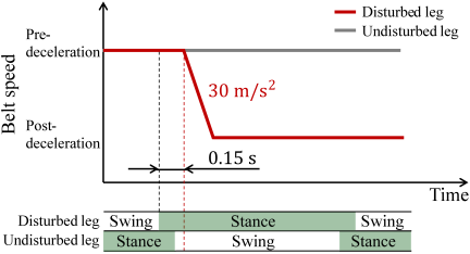
Fig. 3. Gait cycle and belt speed on the perturbation side.
First, during normal walking before the application of a disturbance, the same value is commanded to both the left and right sides. Next, shortly after the decelerating leg touches the ground, the post-deceleration value is commanded to only the decelerating leg. This acts as a mechanical disturbance on the supporting leg. The speed difference was determined to be small enough to allow the subject to continue walking without falling, but large enough to induce a postural response to the disturbance. The time from touch down to the start of deceleration is determined as the time when the large COP fluctuations caused by the impact of the legs with the ground at touchdown converged as shown in Fig. 4. In addition, the belt speed indication during deceleration is set to a step-like manner.
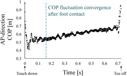
Fig. 4. AP-direction COP during stance phase at comfortable walking speed. AP refers to the anterior–posterior direction.
2.3. Posture Recovery Identification Method
This section explains a method for system identification of human postural control ability during walking as a mathematical model. The section derives a mathematical model based on COP fluctuations, which represent the relatively small postural response caused by disturbances due to treadmill belt deceleration.
The postural response dynamics to large mechanical disturbances that can lead to falls during walking is inherently considered to be nonlinear dynamics and time-varying systems. However, previous research (citing Togoe et al.’s paper 15) has shown that, with relatively small disturbance inputs, if appropriate COP input data for a short period representing the attitude change corresponding to that dynamic disturbance is available, the attitude correction capability can be fairly well represented by a linear system approximation. Therefore, we assume a linear input–output system and consider a discrete-time linear time-invariant system that generally represents this. We apply the least squares method using the Auto Regression eXogenous (ARX) model, which is commonly used for identifying discrete-time linear time-invariant systems.
The discrete-time state equation of the ARX model is expressed as follows:
First, we find the coefficients of the numerator and denominator polynomials.
From Eqs. (3) and (7), \(\boldsymbol{A}\) is composed of output data \(y\) and input data \(u\), and from Eq. (6), \(\boldsymbol{y}\) is the output data itself. Therefore, the coefficient vector \(\boldsymbol{c}\) can be calculated from Eq. (12). Then, we obtain a transfer function, which is a dynamics model, using the coefficient vector \(\boldsymbol{c}\). Assuming \(r_t=0\), and performing the \(\mathcal{Z}\) transformation for \(y_k\),
2.4. How to Select the Order of the System
To obtain the transfer function of the system to be identified, the order of the transfer function \(N, M\) in Eq. (14) must be selected in advance. It is difficult to determine the order that can adequately represent the attitude control dynamics before identification. Furthermore, if the order is too small, the attitude control dynamics cannot be adequately represented, which may result in insufficient identification accuracy. On the other hand, if the order is too large, overfitting may occur to various errors, such as COP measurement errors, which may result in insufficient identification accuracy.
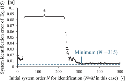
Fig. 5. Relationship between system order and identification error.
Therefore, while changing the order \(N, M\), the error between the experimental COP response \(y_{i, \mathrm{actual}}\) and the response \(y_{i, \mathrm{simulation}}\) calculated from the identification model using the same input data is calculated using the following formula:
2.5. Evaluation of Posture Recovery Ability Using Poles of the Transfer Function
As shown in Section 2.3, the method allows the numerator and denominator of the transfer function to be obtained as rational polynomials, and the roots, i.e., the poles and zeros, can be calculated using numerical solutions. When this transfer function is proper,
In a real response, poles close to the origin decay rapidly as the time step progresses, and therefore have less effect on the output. On the other hand, poles close to the unit circle are less damped as the time step advances and become dominant in the output. Therefore, the following index \(S\), which takes into account the poles after \(K\) steps as a weighting for poles close to the unit circle, is considered as an index of posture recovery ability in this study.
As mentioned in Section 2.3, this method is thought to simultaneously estimate the poles of the dynamics specific to normal walking. The poles related to the dynamics corresponding to posture recovery from mechanical disturbances during walking are considered important. Therefore, as shown in Fig. 6, only poles whose argument \(\theta\) is within a specific range are used to calculate the index. The pole angle \(\theta\) corresponds to the frequency component of the output \(y\), and we select poles with angles corresponding to the frequency bands where the characteristics of posture recovery dynamics have been confirmed through frequency analysis, which means frequency filtering for poles. The pole angle \(\theta\) [deg] and the output frequency \(f\) [Hz] are related as follows:
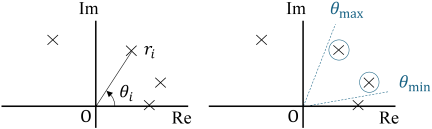
Fig. 6. Selection of poles for evaluation restricted by their angular position.
3. Experiments to Confirm the Validity of the Proposed Method
This section describes experiments conducted to verify whether the proposed method can appropriately evaluate posture recovery ability during walking. We conduct a disturbance response experiment for each same participant under two conditions where their postural recovery ability is intentionally low and normal. We then verify whether the proposed method can clearly express quantitative differences under the two conditions.
The appearance of the equipment used in this experiment is shown in Fig. 7. This experiment is conducted with the approval of the Kyushu University Faculty of Engineering Experimental Ethics Review Committee (approval number: Engineering Approval 2025-06). The treadmill (Bertec, ITR5018-11) used in this experiment consists of two separate belts, one on the left and one on the right. In the treadmill, force plates capable of measuring ground reaction forces are installed under each belt, which is used to calculate output response \(y\) (COP).
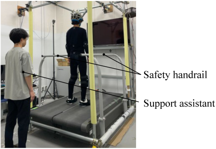
Fig. 7. Exterior of split belt treadmill.
Walking events are detected by referencing the vertical component of the ground reaction force measured by the force plate. The threshold for determining foot contact is set to 15 N. The input for system identification is the belt speed difference, which requires accurate speed measurement. For this purpose, the treadmill belt speed is measured directly using a rotary encoder attached to the wheel (Fig. 8).
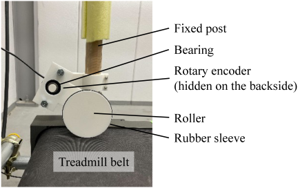
Fig. 8. Encoder-equipped roller fabricated for belt speed measurement.
3.1. Experiment and Measurement
Participants walk at a constant, self-selected comfortable walking speed on the treadmill. As a disturbance during walking, only one side of the belt is suddenly decelerated. At that point, the participant must suddenly decelerate the speed of the leg that is standing on that belt, which becomes a mechanical disturbance. A schematic diagram of treadmill belt deceleration is shown in Fig. 3. The time from the start of the stance phase to the start of deceleration is determined based on preliminary experiments, which is explained in Section 2.2. The participants are asked to walk at a comfortable speed, and COP fluctuations during normal walking were measured. An example is shown in Fig. 4. Sampling time \(T=1\) ms is used in the experiment. These results allowed us to estimate the point at which the large COP fluctuations caused by normal walking during heel strike converge to some extent, and we set the timing of applying artificial disturbance input due to treadmill speed differences to 0.15 s after this point.
This allows for some degree of separation of the influence of postural response dynamics caused by normal walking. Furthermore, even when using COP response data that include some dynamics for normal walking, it is believed that the proposed method can still be used to evaluate postural correction ability.
3.2. COP Measurement with Different Postual Recovery Ability Conditions
To confirm whether the proposed method can quantitatively evaluate the apparent decline in postural control ability alone, we conducted experiments by four participants under conditions in which postural recovery ability was artificially reduced and under normal walking conditions for each.
During walking, the sole of the foot is the only part of contact with the environment, and postural control via the sole is essential for maintaining stable walking 20. Therefore, we set two conditions to evaluate posture recovery ability: one in which a marble (sphere) is held between the toes and one in which it is not held. Fig. 9 shows the results of measurements of plantar pressure distribution and COP trajectory for participant A when walking without holding a marble and when walking with a marble held between his toes. The green area in the figure represents the part where the sole of the foot touches the ground during walking, and the white line segment shows the COP trajectory. By comparing the cases with and without a marble clamp, it can be seen that when a marble is clamped, the contact with the toes, especially the area around the big toe, disappears. These results suggest that the action of holding the marble between the toes inhibits the toes from stepping on or pushing off the ground. Therefore, the use of marbles in this experiment is considered to be a valid condition for intentionally reducing posture recovery ability.
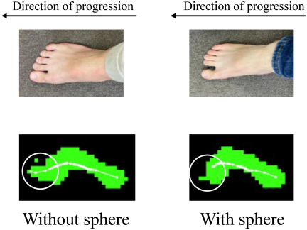
Fig. 9. Comparison of foot contact areas between the non‑grasping and grasping conditions using a small hard sphere.
3.3. Time-Frequency Analysis of COP Fluctuations
Figure 10 shows the time-frequency analysis of COP fluctuations for a representative trial of participant A. The figure shows frequency on the vertical axis, time on the horizontal axis, and gain as color intensity. Note that the time window length was set to 0.128 s, so the 0.064 s at both ends are blank. In the figures, (i) shows the time-frequency distribution during a normal walking cycle without disturbances due to belt speed differences, and (ii) shows the time-frequency distribution when disturbances due to belt speed differences are applied from 0.15 s after ground contact.
The gain is particularly different in the areas marked with black squares, from 0 Hz to 40 Hz and from 0.15 s to 0.5 s, indicating that the frequency characteristics are different. From the result, it is predicted that different dynamics are excited before and during belt deceleration. In particular, for this part, the dynamics during belt deceleration (ii) was considered as the attitude control dynamics in response to disturbances, and system identification was performed.
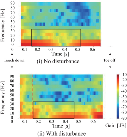
Fig. 10. Time-frequency analysis of COP for subject A.
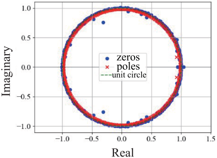
Fig. 11. Distribution of poles of the transfer function for subject A.
The postural control dynamics in response to belt deceleration, which differs from the dynamics of normal walking before belt deceleration, was identified as a transfer function using the method described in the previous section, where the system order \(N=315\) (\(=M\)) is selected by the optimization in Section 2.4. In this case, the time interval for the input/output data used for identification is set to 350 ms from the start of belt deceleration, based on the results of Fig. 10 in this section.
An example of the pole distribution of the identified transfer function is shown in Fig. 11. Note that in discrete linear models, stable poles lie within the unit circle, and the distance from the origin indicates the speed of convergence, i.e., how quickly the orientation converges.
3.4. Calculation of Posture Recovery Performance Evaluation Index
For each participant, we confirmed that there was a difference in the evaluation index of postural control ability defined by Eq. (22) between the experimental conditions in which the marble was sandwiched and the experimental conditions in which it was not sandwiched. Based on the results in Section 2.5, the poles used for evaluation were determined to have angles between 0.1 Hz and 40 Hz. Therefore, from Eq. (23), \(\theta_\mathrm{min}=0.036°\), \(\theta_\mathrm{max}=14.4°\). The values of the evaluation indices for each participant are shown in Figs. 12–15. A significant difference in the value of the evaluation index \(S\) was confirmed between the two experimental conditions for all four participants, demonstrating that this method can quantitatively determine postural recovery ability.
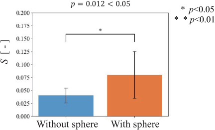
Fig. 12. Comparison of the evaluation metric \(S\) between the two conditions: without bead and with bead for subject A. \(S\) is the stability index, where a larger value indicates a lower risk of falling.
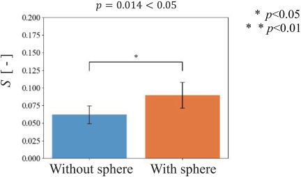
Fig. 13. Comparison of the evaluation metric \(S\) between the two conditions: without bead and with bead for subject B. \(S\) is the stability index, where a larger value indicates a lower risk of falling.
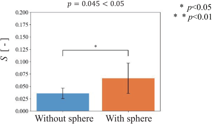
Fig. 14. Comparison of the evaluation metric \(S\) between the two conditions: without bead and with bead for subject C. \(S\) is the stability index, where a larger value indicates a lower risk of falling.
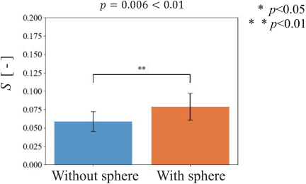
Fig. 15. Comparison of the evaluation metric \(S\) between the two conditions: without bead and with bead for subject D. \(S\) is the stability index, where a larger value indicates a lower risk of falling.
4. Conclusion
This paper proposed a disturbance application method and disturbance response experiments using a left-right separated treadmill to extract the postural control dynamics during human walking, and proposed a quantitative evaluation method for postural recovery ability during walking based on system identification.
To confirm the validity of the proposed method, we set two experimental conditions that clearly differed in posture recovery ability and conducted a disturbance application experiment with four participants. Analysis of the experimental data confirmed high reproducibility of COP fluctuations in response to disturbances. Time-frequency analysis confirmed temporal changes in frequency characteristics before and after the application of disturbances. This confirmed that the proposed method appropriately excites posture control dynamics. Comparing the evaluation indices between the presence and absence of holding a marble between the toes, we showed that the two conditions could be significantly distinguished. These results demonstrate that the method for identifying disturbance response dynamics during human walking is effective as an index for evaluating postural recovery performance.
The proposed method is based on a system identification method under the assumption of a linear system, and does not assume large disturbance inputs that would lead to inversion. However, this method allows for the quantitative evaluation of a person’s basic postural recovery ability in the event of minor disturbance inputs, and it is believed that this basic ability can be appropriately evaluated even during walking using the proposed method. Furthermore, providing clearly different postural recovery capabilities as experimental conditions is important for verifying its usefulness. This method is thought to be applicable to other gait stability evaluation methods during walking.
Acknowledgments
This study was supported by JSPS KAKENHI (Grant Number: 24K03323, 25K03507).
- [1] S. M. Thomas, A. Parker, J. Fortune, G. Mitchell, A. Hezam, Y. Jiang, M. de Groh, K. Anderson, A. Gauthier-Beaupré, J. Barker, J. Watt, S. E. Straus, and A. C. Tricco, “Global evidence on falls and subsequent social isolation in older adults: A scoping review,” BMJ Open, Vol.12, No.9, Article No.e062124, 2022. https://doi.org/10.1136/bmjopen-2022-062124
- [2] A. Gabell, M. A. Simons, and U. S. Nayak, “Falls in the healthy elderly: Predisposing causes,” Ergonomics, Vol.28, No.7, pp. 965-975, 1985. https://doi.org/10.1080/00140138508963219
- [3] Y. Cai, S. G. Leveille, O. Andreeva, L. Shi, P. Chen, and T. You, “Characterizing fall circumstances in community-dwelling older adults: A mixed methods approach,” J. Gerontol. A Biol. Sci. Med. Sci., Vol.78, No.9, pp. 1683-1691, 2023. https://doi.org/10.1093/gerona/glad130
- [4] N. Niino, S. Tsuzuku, F. Ando, and H. Shimokata, “Frequencies and circumstances of falls in the national institute for longevity sciences, longitudinal study of aging (NILS-LSA),” J. of Epidemiology, Vol.10, No.1 Suppl, pp. S90-S94, 2000. https://doi.org/10.2188/jea.10.1sup_90
- [5] S. Mathias, U. Nayak, and B. Isaacs, “Balance in elderly patients: The “get-up and go” test,” Archives of Pysical Medicine and Rehabilitation, Vol.67, No.6, pp. 387-389, 1986.
- [6] D. Podsiadlo and S. Richardson, “The timed “up & go”: A test of basic functional mobility for frail elderly persons,” J. of the American Geriatrics Society, Vol.39, No.2, pp. 142-148, 1991. https://doi.org/10.1111/j.1532-5415.1991.tb01616.x
- [7] K. Berg, S. Wood-Daupinee, J. Williams, and D. Gayton, “Measuring balance in the elderly: Preliminary development of an instrument,” Physiotherapy Canada, Vol.41, No.6, pp. 304-311, 1989.
- [8] M. Tinetti, “Performance-oriented assessment of mobility problems in elderly patients,” J. of the American Geriatrics Society, Vol.34, No.2, pp. 119-126, 1986.
- [9] D. Martelli, F. Aprigliano, P. Tropea, G. Pasquini, S. Micera, and V. Monaco, “Stability against backward balance loss: Age-related modifications following slip-like perturbations of multiple amplitudes,” Gait & Posture, Vol.53, pp. 207-214, 2017. https://doi.org/10.1016/j.gaitpost.2017.02.002
- [10] L. Hak, H. Houdijk, F. Steenbrink, A. Mert, P. van der Wurff, P. J. Beek, and J. H. van Dieën, “Speeding up or slowing down?: Gait adaptations to preserve gait stability in response to balance perturbations,” Gait & Posture, Vol.36, No.2, pp. 260-264, 2012. https://doi.org/10.1016/j.gaitpost.2012.03.005
- [11] C. McCrum, G. Epro, K. Meijer, W. Zijlstra, G. P. Brüggemann, and K. Karamanidis, “Locomotor stability and adaptation during perturbed walking across the adult female lifespan,” J. of Biomechanics, Vol.49, No.7, pp. 1244-1247, 2016. https://doi.org/10.1016/j.jbiomech.2016.02.051
- [12] A. Hof, M. Gazendam, and W. Sinke, “The condition for dynamic stability,” J. of Biomechanics, Vol.38, No.1, pp. 1-8, 2005. https://doi.org/10.1016/j.jbiomech.2004.03.025
- [13] H. Watanabe, S. Okamoto, T. Kuroda, and Y. Akiyama, “Manipulability analysis of anterior and mediolateral dynamic gait stability of young and elderly individuals,” J. Robot. Mechatron., Vol.36, No.6, pp. 1568-1576, 2024. https://doi.org/10.20965/jrm.2024.p1568
- [14] T. Miyazaki, T. Aoki, J. Aizawa, T. Kawase, M. Sogabe, and K. Kawashima, “Adapting balance training by changing the direction of the tensile load on the lumbar region,” J. Robot. Mechatron., Vol.34, No.6, pp. 1361-1370, 2022. https://doi.org/10.20965/jrm.2022.p1361
- [15] T. Togoe, P. H. Tung, Y. Nakashima, and M. Yamamoto, “An evaluation method of human standing stability by applying the disturbance of swash plate fall,” Trans. of the JSME, Vol.87, No.896, Article No.20-00302, 2021 (in Japanese). https://doi.org/10.1299/transjsme.20-00302
- [16] M. Schimpl, C. Moore, C. Lederer, A. Neuhaus, J. Sambrook, J. Danesh, W. Ouwehand, and M. Daumer, “Association between walking speed and age in healthy, free-living individuals using mobile accelerometry—A cross-sectional study,” PLoS ONE, Vol.6, No.8, Article No.e23299, 2011. https://doi.org/10.1371/journal.pone.0023299
- [17] B. J. Loyd, J. Saviers-Steiger, A. Fangman, S. S. Paul, P. C. Fino, M. E. Lester, and L. E. Dibble, “Control of linear head and trunk acceleration during gait after unilateral vestibular deficits,” Archives of Physical Medicine and Rehabilitation, Vol.102, No.3, pp. 456-462, 2021. https://doi.org/10.1016/j.apmr.2020.08.005
- [18] T. Boerger, J. V. Dehy, T. Onushko, B. Schmit, and A. Hyngstrom, “Step length and width variability while walking on a motion simulator mounted treadmill,” Proc. of the 2016 38th Annual Int. Conf. of the IEEE Engineering in Medicine and Biology Society (EMBC), pp. 4577-4580, 2016. https://doi.org/10.1109/EMBC.2016.7591746
- [19] D. A. Winter, “Human balance and posture control during standing and walking,” Gait & Posture, Vol.3, No.4, pp. 193-214, 1995. https://doi.org/10.1016/0966-6362(96)82849-9
- [20] A. M. van Leeuwen, J. H. van Dieën, A. Daffertshofer, and S. M. Bruijn, “Ankle muscles drive mediolateral center of pressure control to ensure stable steady state gait,” Scientific Reports, Vol.11, No.1, Article No.21481, 2021. https://doi.org/10.1038/s41598-021-00463-8
- [a] World Health Organization, “Falls,” 2021. https://www.who.int/news-room/fact-sheets/detail/falls [Accessed November 19, 2025]
This article is published under a Creative Commons Attribution-NoDerivatives 4.0 Internationa License.