
Paper:
Observable Point Cloud Maps for Wide-Area Self-Localization
Kazuma Yagi, Shugo Nishimura, Yu Okita, Photchara Ratsamee
 , Kazuyo Tsuzuki
, Seiji Aoyagi
, and Yasushi Mae†
, Kazuyo Tsuzuki
, Seiji Aoyagi
, and Yasushi Mae†
Kansai University
3-3-35 Yamate-cho, Suita, Osaka 564-8680, Japan
†Corresponding author

Self-localization using a pre-constructed point cloud map is effective even in global navigation satellite system-denied settings, such as indoor environments and areas adjacent to buildings. In wide-area environments, however, the amount of map data becomes enormous, increasing storage and computational costs. This study proposes a method to partition a wide-area point cloud map into local regions and construct observable point cloud maps by extracting only the points observable from virtual viewpoints placed within each region. Each observable point cloud map contains only the point cloud that contributes to self-localization in the corresponding local region. During the self-localization process, the robot dynamically switches the observable point cloud maps according to its current local region. Self-localization accuracy and computational costs are evaluated using both the wide-area point cloud map and proposed observable point cloud maps. Additionally, the localization contribution per point is used to quantify the effectiveness of the retained map points. The results show the dynamic switching of observable point cloud maps enables memory-efficient self-localization while maintaining localization accuracy comparable to that of the wide-area point cloud map.
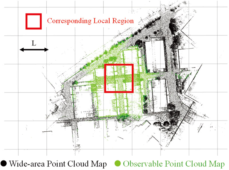
Observable point cloud map
1. Introduction
Accurate and robust self-localization is essential for autonomous mobile robots to operate reliably in diverse indoor and outdoor environments 1,2. Although global navigation satellite system-based localization is commonly used outdoors, its accuracy significantly degrades around tall buildings or inside structures due to signal blockage and multipath effects 3. In such environments, self-localization via map-matching using depth sensors, such as LiDAR, and a pre-constructed 3D point cloud map is widely adopted and highly effective 4,5.
Self-localization using a 3D point cloud map is versatile because it directly utilizes the geometric structure of the environment. Recent studies have focused on accelerating scan matching, including range-image-based localization 6, voxelized generalized iterative closest point for reducing correspondence searches 7, and robust registration combining inertial measurement unit (IMU) preintegration with feature extraction 8. However, these methods typically assume a large-scale point cloud map, which can contain tens of millions of points in wide-area environments. Consequently, scan matching that relies on sequentially referencing the entire map still faces heavy computational costs for correspondence searches and spatial queries 9,10.
To address this issue, several map compression and lightweight representation techniques have been proposed for wide-area point cloud maps. Examples include teacher–student compression models that reduce map size while preserving accuracy 11, studies analyzing compressibility for efficient map representation in registration tasks 12, and deep-learning-based geometric compression methods 13. However, these methods operate on the entire map in a unified representation and do not consider the robot’s field-of-view constraints or dynamically switch maps according to traversable regions. As a result, structures that are never observed from the robot’s trajectory or lie outside the sensor’s field of view may remain in the map, potentially leading to incorrect correspondences or increased search times during scan matching.
In this study, we propose a method to partition a wide-area point cloud map into local point cloud maps, each consisting of points that are observable from virtual viewpoints placed on traversable areas within that map region. We call this the observable point cloud map. During self-localization, the proposed method dynamically switches between the observable point cloud maps according to the robot’s current local region. The robot refers only the observable point cloud map corresponding to its current local region to reduce the number of map points while maintaining localization accuracy. The effectiveness of the retained map points is evaluated using the localization contribution per point (LCP) to enable a quantitative comparison between the wide-area point cloud map and proposed observable point cloud maps 14.
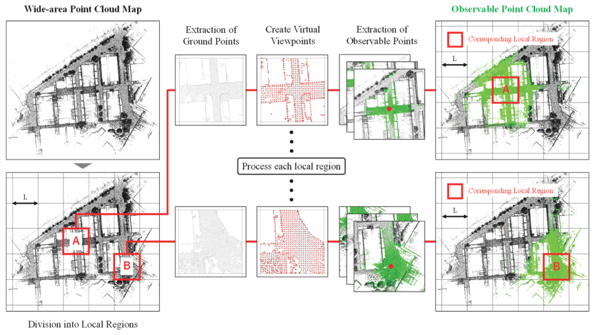
Fig. 1. Concept of the local-region observable point cloud map.
2. Self-Localization by Observable Point Cloud Maps
In this section, we describe the procedure for generating observable point cloud maps for each local region from a wide-area point cloud map, as well as the self-localization process through dynamic map switching. The proposed method partitions the environment into local regions and extracts observable points. For each region, only the points that can actually be observed from virtual viewpoints placed within traversable areas are retrained. A conceptual overview of the method is shown in Fig. 1, where a uniform grid is used to partition the wide-area point cloud map into local regions. The process of constructing observable point cloud maps for two local regions (A and B) is illustrated, and the resulting observable point cloud maps are represented by green points.
We assume that a wide-area point cloud map containing ground points is provided in advance, and that the robot is equipped with a depth sensor (LiDAR) capable of 3D measurements. The proposed method is based on the assumptions that the traversable area corresponds to the ground surface and that localization is performed in static environments. Dynamic obstacles and temporal map changes are not explicitly considered. Furthermore, a uniform grid partitioning scheme is adopted in this study, although it is not necessarily optimal in all environments. As input, we use the wide-area point cloud map \(\mathcal{P}\) expressed in a global coordinate frame as:
-
Partitioning of the wide-area map into local regions
-
Virtual viewpoint generation in each local region
-
Extraction of observable points and construction of observable point cloud maps
-
Dynamic switching of observable point cloud maps during self-localization
The details of each step are described below.
2.1. Partitioning of the Wide-Area Map into Local Regions
To enable local self-localization, the wide-area map is partitioned into local regions. We adopt a uniform grid as the basis for partitioning, where each local region is defined as a grid cell with width \(L\). Let \(( x_{min},y_{min} )\) denote the origin of partitioning. The grid cell \(\mathcal{G}_{ij}\) is defined as
The set of points \(\mathcal{P}_{ij}\) contained in the grid cell \(\mathcal{G}_{ij}\) is defined by
2.2. Virtual Viewpoint Generation in Each Local Region
For each local region, virtual viewpoints representing possible robot perspectives are generated. The traversable area of the robot is assumed to correspond to the ground surface within the environment. Ground points are first extracted from the wide-area point cloud map, and representative points of the ground are used as virtual viewpoints.
Ground extraction is performed using the progressive morphological filter (PMF) 15, yielding a ground point set \(g_{ij}\subset \mathcal{P}_{ij}\). The PMF gradually enlarges the window size to estimate the ground surface, enabling robust extraction even in environments with smooth elevation changes, while remaining computationally efficient for large-scale point cloud maps. The proposed method is not dependent on a specific ground extraction technique; alternative ground segmentation methods may also be applied.
Representative points are obtained by applying a voxel grid filter to the extracted ground points. Let \(s_{voxel}\) denote the voxel size, \(g_{ij}\) denote the set of ground points in grid cell \(\mathcal{G}_{ij}\), and \(g_{ij}^{\left(m \right)}\) denote the subset of ground points contained in voxel \(m\). The representative point \(\hat{\boldsymbol{q}}_{ij,m}\) of voxel \(m\) is defined as
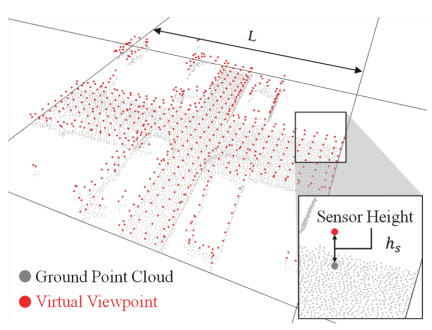
Fig. 2. Concept of virtual viewpoint placement within a grid.
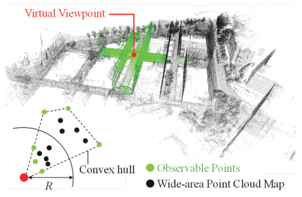
Fig. 3. Concept of visibility determination.
2.3. Extraction of Observable Points and Construction of Observable Point Cloud Maps
Observable points are defined as points that are directly visible from a single viewpoint, considering occlusions in the surrounding environment. For each virtual viewpoint \(\boldsymbol{q}_{ij,m}\), the observable points are extracted from the wide-area point cloud map \(\mathcal{P}\). To obtain these points, the hidden point removal (HPR) operator is employed 16. By integrating the observable points extracted for all virtual viewpoints within a local region \(\mathcal{G}_{ij}\), the observable point cloud map for that region is constructed. HPR operates by first translating the point cloud so that the viewpoint becomes the origin and then applying a spherical inversion. Computing the convex hull of inverted points identifies corresponding original points, which are then classified as observable.
The observable check process is as follows. The HPR radius \(R\) is set proportional to the diagonal length \(D\) of the bounding box enclosing the wide-area point cloud map, where \(\alpha\) is a positive constant:
The observable point cloud map \(\mathcal{V}_{ij}\) for the local region \(\mathcal{G}_{ij}\) is then obtained as the union of the observable point sets from all virtual viewpoints in that region:
The observable point cloud maps generated for each local region are stored independently and are dynamically switched during self-localization based on the robot’s current position.
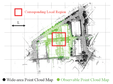
Fig. 4. Example of the generated observable point cloud map.
2.4. Dynamic Switching of Observable Point Cloud Maps During Self-Localization
During self-localization, the estimated robot position \(( x_{t},y_{t} )\) at time \(t\) is obtained by scan matching. Based on this position, the local region to which the robot belongs is determined, and only the corresponding observable point cloud map is used as the local map. If the determined region remains the same, the current point cloud map is retained for the next scan matching. If a different region is identified, the corresponding point cloud map is loaded and used for the next iteration. This process is referred to as map switching.
Because local regions are represented as grid cells in this study, let \(L\) denote the grid width and \(( x_{min},y_{min} )\) denote the origin of grid partitioning. The grid index \(( u_{t},v_{t})\) corresponding to the robot’s position is computed as:
The observable point cloud map \(\mathcal{V}_{u_{t}v_{t}}\) associated with the identified local region \(\mathcal{G}_{u_{t}v_{t}}\) is then loaded and used for scan matching. A conceptual illustration of this process is shown in Fig. 5.
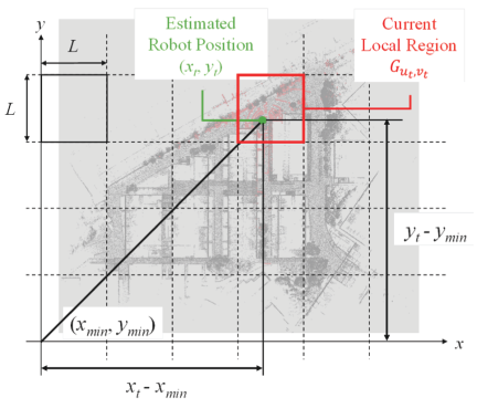
Fig. 5. Determination of the robot’s local region.
Because map switching occurs only when the robot crosses a local-region boundary, the number of point-cloud loads increases linearly with the travel distance, eliminating the need to retain entire wide-area point cloud map in memory. Consequently, the number of points used for scan matching is significantly reduced, thereby reducing the cost of correspondence search and improving computational efficiency.
3. Experiment
In this study, self-localization is performed using both the wide-area and observable point cloud maps generated by the proposed method. The computation time and localization accuracy are compared to evaluate the effectiveness of the proposed approach. Additionally, LCP is employed as an index to quantify the contribution of each map point to the localization accuracy.
3.1. Experimental Environment
3.1.1. Autonomous Mobile Robot “KUAMS”
The mobile robot used in this study is “KUAMS,” an autonomous navigation platform developed at Kansai University. The platform is based on the personal mobility vehicle WHILL Model CR manufactured by WHILL Inc., which was modified for research purposes.
A 3D LiDAR sensor (Velodyne VLP-16) is mounted horizontally at the top of the robot at a height of 1 m above the ground. The sensor provides a vertical field of view from \(-\)15° to \(+\)15° and a full 360° horizontal field of view. The VLP-16 offers a measurement range up to 100 m with a typical distance accuracy of m. At a rotation frequency of 10 Hz, the vertical and horizontal angular resolutions are approximately 2° and 0.2°, respectively.
Control and point cloud processing were performed on an onboard laptop PC equipped with an Intel Core i7-12700H CPU and 16 GB of RAM, running Ubuntu 22.04 LTS. The proposed method and localization algorithms were implemented in C\(++\) using ROS 2 Humble. The appearance of the robot is shown in Fig. 6.
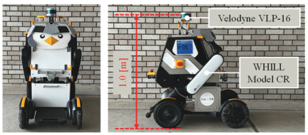
Fig. 6. External appearance of the KUAMS.
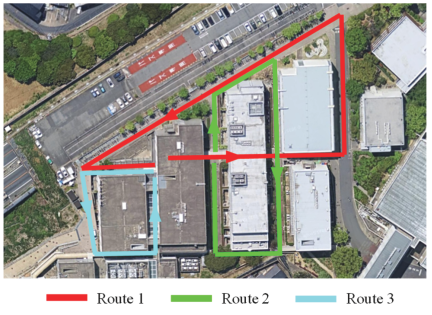
Fig. 7. Experimental route layout.
3.1.2. Experimental Site
The experiments were conducted in the wide-area environment surrounding the buildings at Kansai University, as shown in Fig. 7. To ensure the robot’s operational area was fully covered by the wide-area point cloud map, three distinct routes were defined within the environment. The robot was driven along each route to collect the required sensor data.
3.2. Experimental Preparation
3.2.1. Construction of the Wide-Area Point Cloud Map
To construct the wide-area point cloud map, globally consistent local implicit mapping (GLIM) 17—a LiDAR–IMU fusion simultaneous localization and mapping (SLAM) method—was employed. GLIM incrementally generates local submaps and subsequently integrates and optimizes them in a globally consistent manner, enabling the creation of a highly accurate and low-drift 3D map of a large environment.
The sensor data used for mapping comprised 3D LiDAR measurements and inertial data obtained from a Livox MID-360 sensor. The resulting wide-area point cloud map is shown in Fig. 8.
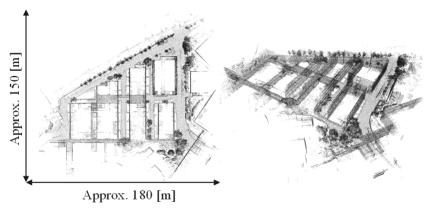
Fig. 8. Constructed wide-area point cloud map.
3.2.2. Construction of Observable Point Cloud Maps
Observable point cloud maps were generated for each local region from the wide-area point cloud map using the proposed method. Because the grid size used for local-region partitioning affects both the density of the observable point cloud maps and computational load of self-localization, three representative grid widths were selected. These sizes were used to evaluate the influence of partitioning on localization accuracy and processing time. The experimental parameters are summarized below:
- • \(L=\)10.0 m, 20.0 m, 30.0 m
-
Grid size for local-region partitioning in Section 2.1.
- • \(s_{voxel}=1.0\) m
-
Voxel size for generating virtual viewpoints in Section 2.2.
- • \(h_{s}=1.0\) m
-
Sensor height used in virtual viewpoint modeling in Section 2.2.
- • \(\alpha =100.0\) [-]
-
Proportional coefficient for determining the HPR radius in Section 2.3.
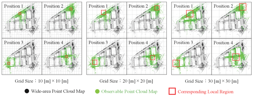
Fig. 9. Comparison of the generated observable point cloud maps.
3.3. Experimental Method
Self-localization was performed using the wide-area point cloud and observable point cloud maps generated by the proposed method. LiDAR data collected along the three predefined routes served as the input for this evaluation. We measured the processing time required for scan matching \(T_{\textit{align}}\) and the accuracy metric \(S_{\textit{fitness}}\). Normal distribution transform (NDT) scan matching was employed as the localization method 18, specifically using the ndt_omp implementation a. The metric \(T_\textit{align}\) represents only the processing time for NDT scan matching after the corresponding point cloud map has been loaded into memory. The overhead associated with map switching and disk loading is excluded from \(T_{\textit{align}}\): therefore, the reported processing time reflects the pure alignment cost under the given map. The accuracy metric \(S_{\textit{fitness}}\) represents average similarity between each transformed point and the surrounding voxel distributions, defined as follows:
This metric evaluates how well each transformed point fits the surrounding voxel distributions based on a Gaussian model. The variables in the aforementioned equation are defined as follows:
-
\(N\): Number of points in the transformed point cloud,
-
\(N_{i}\): Set of neighboring voxels associated with point \({x'}_{i}\),
-
\({x'}_{i}\): The \(i\)-th point after transformation,
-
\(\mu_{j}\): Mean position vector of voxel \(j\),
-
\(\sum_{j}^{-1}\): Inverse covariance matrix of voxel \(j\),
-
\(d_{1},d_{2},d_{3}\): NDT score coefficients 19.
The NDT score coefficients were determined within the ndt_omp implementation based on the outlier ratio and voxel resolution. In this experiment, we set the parameters as \(d_{1}=0.00354\), \(d_{2}=0.432\), and \(d_{3}=-2.74\). These parameters quantify the consistency between each point and its neighboring voxel distributions, where higher values indicate better alignment.
3.4. Evaluation Method
The effectiveness of the proposed method was evaluated using the metrics described in Section 3.3. Specifically, to quantitatively assess the contribution of each map point to self-localization, the LCP was employed. LCP is defined using the number of map points \(N_{point}\) used for localization and the accuracy metric \(S_{\textit{fitness}}\) as:
4. Experimental Results and Discussion
Table 1. Comparison of point counts.
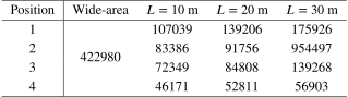
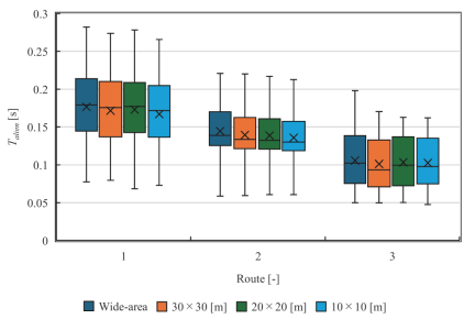
Fig. 10. Point cloud alignment time.
Examples of the observable point cloud maps generated for the three selected grid widths are shown in Fig. 9, and the number of points in each observable point cloud map is summarized in Table 1. As expected, smaller grid sizes result in a significantly lower number of points within each local region. This reduction occurs because finer partitioning extracts only the local structures observable by the robot at a given location, while redundant or distinct points are effectively filtered out.
Self-localization was performed using the LiDAR data collected along each route. The resulting processing time \(T_{\textit{align}}\) and accuracy metric \(S_{\textit{fitness}}\) are presented in Figs. 10 and 11, respectively. As shown in Fig. 10, the alignment time \(T_{\textit{align}}\) remains nearly constant across different grid sizes and is comparable to that of the wide-area point cloud map. Although slight variations can be observed, all configurations operate within a similar real-time range. This indicates that the proposed method maintains stable real-time performance while substantially reducing the number of map points.
On the other hand, the results for \(S_{\textit{fitness}}\) in Fig. 11 indicate that all grid sizes achieved an accuracy comparable to or higher than that of the wide-area point cloud map. This improvement occurs because the proposed method extracts only the observable points within each local region, effectively removing occluded structures or points behind obstacles that do not contribute to localization. By reducing false correspondences and retaining only the locally consistent points, the scan matching process achieves stable alignment quality, resulting in comparable or slightly improved \(S_{\textit{fitness}}\).
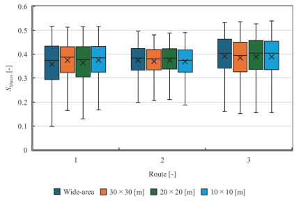
Fig. 11. Scan-matching fitness score.
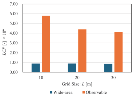
Fig. 12. LCP.
Figure 12 shows the average LCP for each grid size. Across all grid sizes, LCP was consistently higher than that obtained using the wide-area point cloud map. This demonstrates that observable point cloud maps retained only the points effective for localization, thereby increasing the relative contribution of each point. Notably, LCP increases as the grid size decreases. With finer grid partitioning, the observable point cloud map for each region more precisely reflects the structures surrounding the robot’s actual position, emphasizing the most informative points. Consequently, the resulting map becomes increasingly composed of points that directly support localization, leading to higher per-point contribution.
Overall, these results indicate that the proposed method enables self-localization that effectively captures the environment on a local scale. By extracting only the points observable from the robot’s viewpoint in each local region, the method constructs a local map that is both efficient and accurate for scan matching. Therefore, using observable point cloud maps enables memory-efficient localization while maintaining real-time performance and high localization accuracy.
5. Conclusion
This study presented a method for self-localization using observable point cloud maps by partitioning a wide-area point cloud map into local regions. Each local point cloud map consists of points observable from virtual viewpoints placed on traversable areas within that region. The proposed approach dynamically switches the observable point cloud maps according to the robot’s current position. This method achieves a significant reduction in the number of map points while maintaining localization accuracy comparable to that of the wide-area point cloud map.
Evaluation based on the LCP confirmed that the observable point cloud maps selectively retained points effective for self-localization.
As future work, although uniform grid partitioning was employed in this study, it is necessary to explore region-partitioning strategies that adaptively optimize the shape of local regions according to environmental structures and robot trajectories. Dynamically adjusting viewpoint density or region boundaries for heterogeneous environments is expected to further improve the efficiency and accuracy of observable point cloud map generation.
Acknowledgments
This work was financially supported in part by the Kansai University Fund for the Promotion and Enhancement of Education and Research, 2023 “Human-centered Life Support for Creating Indoor/Outdoor Well-living Space,” and the Kansai University Grant-in-Aid for progress of research in graduate course, 2025. This work was also supported in part by JSPS KAKENHI Grant Number 25K01205.
- [1] S. Suga, H. Ishii, T. Takahashi, M. Suzuki, K. Tsuzuki, Y. Mae, and S. Aoyagi, “Autonomous navigation of mobile robot based on visual information and GPS—Path planning by semantic segmentation with the A* algorithm and obstacle avoidance by kernel density estimation—,” J. Robot. Mechatron., Vol.37, No.6, pp. 1283-1292, 2025. https://doi.org/10.20965/jrm.2025.p1283
- [2] S. Kurebayashi, T. Tomizawa, and S. Tarao, “Game-engine-based 3D simulation of mobile robot and its application to autonomous navigation in physical environments,” J. Robot. Mechatron., Vol.37, No.6, pp. 1314-1326, 2025. https://doi.org/10.20965/jrm.2025.p1314
- [3] F. Massa, L. Bonamini, A. Settimi, L. Pallottino, and D. Caporale, “LiDAR-based GNSS denied localization for autonomous racing cars,” Sensors, Vol.20, No.14, Article No.3992, 2020. https://doi.org/10.3390/s20143992
- [4] K. Koide, S. Oishi, M. Yokozuka, and A. Banno, “Tightly coupled range inertial localization on a 3D prior map based on sliding window factor graph optimization,” 2024 IEEE Int. Conf. on Robotics and Automation (ICRA), pp. 1745-1751, 2024. https://doi.org/10.1109/icra57147.2024.10611195
- [5] X. Zheng and J. Zhu, “Efficient LiDAR odometry for autonomous driving,” IEEE Robotics and Automation Letters, Vol.6, No.4, pp. 8458-8465, 2021. https://doi.org/10.1109/LRA.2021.3110372
- [6] X. Chen, I. Vizzo, T. Labe, J. Behley, and C. Stachniss, “Range image-based LiDAR localization for autonomous vehicles,” 2021 IEEE Int. Conf. on Robotics and Automation (ICRA), pp. 5802-5808, 2021. https://doi.org/10.1109/icra48506.2021.9561335
- [7] K. Koide, M. Yokozuka, S. Oishi, and A. Banno, “Voxelized GICP for Fast and Accurate 3D Point Cloud Registration,” 2021 IEEE Int. Conf. on Robotics and Automation (ICRA), pp. 11054-11059, 2021. https://doi.org/10.1109/icra48506.2021.9560835
- [8] L. Yang, H. Ma, Z. Nie, H. Zhang, Z. Wang, and C. Wang, “3D LiDAR point cloud registration based on IMU preintegration in coal mine roadways,” Sensors, Vol.23, No.7, Article No.3473, 2023. https://doi.org/10.3390/s23073473
- [9] J. Wen, J. Tang, H. Liu, C. Qian, and X. Fan, “Real-Time Scan-to-Map Matching Localization System Based on Lightweight Pre-Built Occupancy High-Definition Map,” Remote Sensing, Vol.15, No.3, Article No.595, 2023. https://doi.org/10.3390/rs15030595
- [10] S. Aoki, K. Ikeda, and T. Oishi, “Global localization for 3D point cloud scan matching using branch-and-bound algorithm,” arXiv preprint, arXiv:2310.10023, 2023. https://doi.org/10.48550/arXiv.2310.10023
- [11] H. Yin, Y. Wang, L. Tang, X. Ding, S. Huang, and R. Xiong, “3D LiDAR map compression for efficient localization on resource constrained vehicles,” IEEE Trans. on Intelligent Transportation Systems, Vol.22, No.2, pp. 837-852, 2021. https://doi.org/10.1109/tits.2019.2961120
- [12] M.-F. Chang, W. Dong, J. Mangelson, M. Kaess, and S. Lucey, “Map compressibility assessment for LiDAR registration,” 2021 IEEE/RSJ Int. Conf. on Intelligent Robots and Systems (IROS), pp. 5560-5567, 2021. https://doi.org/10.1109/iros51168.2021.9636789
- [13] S. Lu, C. Han, and H. Yang, “Efficient large-scale point cloud geometry compression,” Sensors, Vol.25, No.5, Article No.1325, 2025. https://doi.org/10.3390/s25051325
- [14] K. Yagi, S. Nishimura, T. Matsunaga, K. Tsuzuki, S. Aoyagi, and Y. Mae, “Observable point cloud filtering from travel path for self-localization in wide-area environments,” J. Robot. Mechatron., Vol.37, No.6, pp. 1355-1364, 2025. https://doi.org/10.20965/jrm.2025.p1355
- [15] K. Zhang, S.-C. Chen, D. Whitman, M.-L. Shyu, J. Yan, and C. Zhang, “A progressive morphological filter for removing nonground measurements from airborne LIDAR data,” IEEE Trans. on Geoscience and Remote Sensing, Vol.41, No.4, pp. 872-882, 2003. https://doi.org/10.1109/tgrs.2003.810682
- [16] S. Katz, A. Tal, and R. Basri, “Direct visibility of point sets,” ACM Trans. on Graphics, Vol.26, No.3, Article No.24, 2007. https://doi.org/10.1145/1276377.1276407
- [17] K. Koide, M. Yokozuka, S. Oishi, and A. Banno, “GLIM: 3D range-inertial localization and mapping with GPU-accelerated scan matching factors,” Robotics and Autonomous Systems, Vol.179, Article No.104750, 2024. https://doi.org/10.1016/j.robot.2024.104750
- [18] P. Biber and W. Strasser, “The normal distributions transform: A new approach to laser scan matching,” 2003 IEEE/RSJ Int. Conf. on Intelligent Robots and Systems (IROS 2003), Vol.3, pp. 2743-2748, 2003. https://doi.org/10.1109/iros.2003.1249285
- [19] M. Magnusson, “The three-dimensional normal-distributions transform—An efficient representation for registration, surface analysis, and loop detection,” Ph.D. thesis, Örebro University, 2009.
- [a] K. Koide, koide3/ndt_omp. https://github.com/koide3/ndt_omp [Accessed November 18, 2025]
This article is published under a Creative Commons Attribution-NoDerivatives 4.0 Internationa License.