Paper:
Spontaneous Rhythmic Behavior Generation in Robot Locomotion Based on Mechanical Stabilization
Kai Ito, Keita Sato, and Yusuke Ikemoto

Department of Mechanical Engineering, Faculty of Science and Technology, Meijo University
1-501 Shiogamaguchi, Tempaku-ku, Nagoya, Aichi 486-8502, Japan

Animals exhibit a variety of gait patterns that vary with locomotor speed and energy efficiency. Although a variety of gait patterns have been studied, the mechanism of gait generation has remained vague. In this study, we performed ground reaction force equalization for stable locomotion by developing a one-input, two-output leg-equipped robot with a differential gear. The developed robot can tolerate angular velocity differences and equalize the torque transmitted to the legs. To investigate the possibility of rhythm generation based on ground reaction force equalization, hardware experiments and mathematical analysis were conducted using a nonlinear system. The robot experiments and theoretical analysis show that the robot can spontaneously generate rhythm by equalizing the ground reaction force.
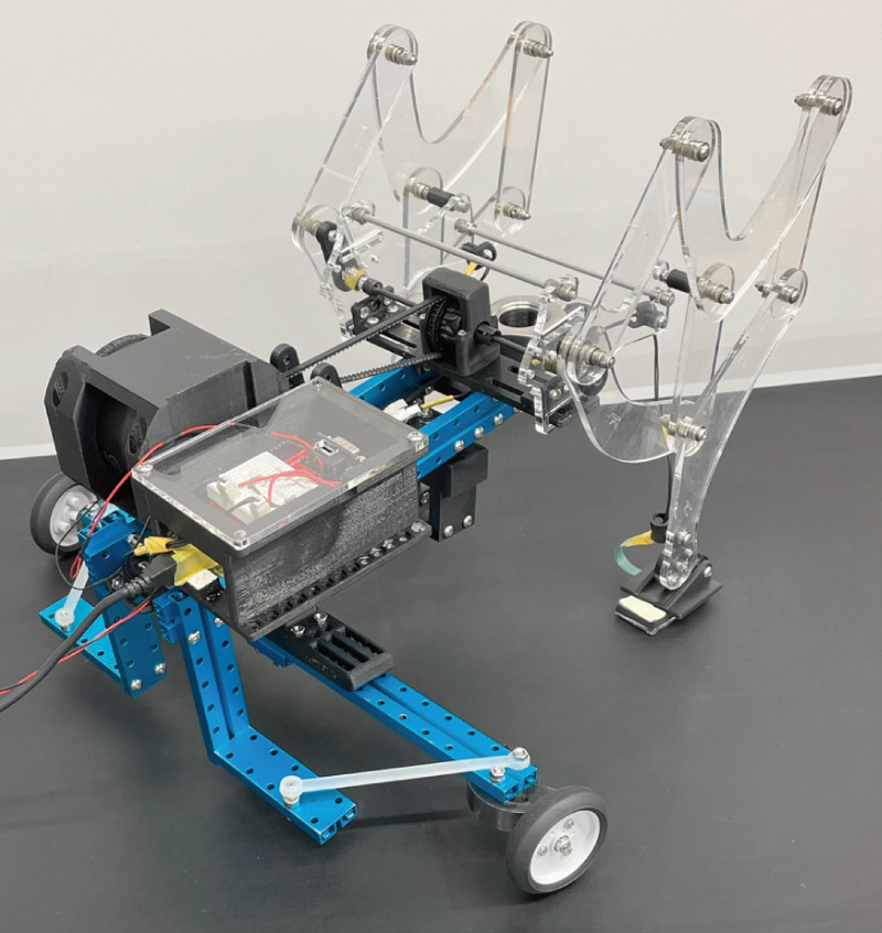
Our robot with differential mechanism
1. Introduction
Animals expanded their range of activities from water to land during the evolutionary process. The ability to move on land was enabled by the possession of legs and the acquisition of rhythmic leg movements. These legged organisms move by rhythmically performing movements that comprise a stance phase in contact with the ground and a swing phase off the ground. Many studies have been conducted on animal gait 1, including mammals 2,3,4, insects 5,6, birds 7. The timing and cycle at which each leg touches the ground are used to describe gait patterns.
Recently, many studies have been conducted on the transition of gait patterns. Crows, which are bipeds, perform “walking” in which the left and right legs alternate, and “hopping” in which the timing of ground contact between the two legs is slightly off 7. Horses, which are quadrupeds, use four gait patterns: walk, trot, canter, and gallop 1. Although these gait patterns are presumed to transition to minimize energy consumption 8,9, the root reason for the gait itself remains unclear. In particular, the internal body mechanics that generate gait remain unclear. Understanding the role of mechanics in rhythm generation may reveal how the motor nervous system, which realizes gait in biology, has developed in collaboration with the mechanical properties because it is determined by the interactions between the body and the ground environment.
In this study, we developed a leg-equipped robot that spontaneously generates gaits through a mechanism that equalizes the ground reaction forces (GRFs) acting on the legs. The equalization of GRFs is achieved by a drive system that transmits equal forces to both legs via a differential mechanism. Unlike conventional robots, in which one or more actuators are assigned to each limb, this drive system has a very simple configuration with only one actuator shared between two limbs. Furthermore, we conducted walking experiments using the physical robot and analyzed its stability characteristics based on nonlinear dynamics. The results suggest that there is the possibility for the mechanism, which maintains postural stability during walking, contributes to the emergence of rhythmic movements. It was also suggested that gait patterns naturally arise from the energy input–output relationship resulting from the interaction between the robot and its environment.
2. Rhythmic Motion in Robots
2.2. Stabilization of Locomotion by Equalizing the Ground Reaction Force
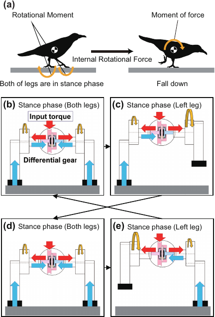
Fig. 1. The balance between GRFs can contribute to stability during locomotion.
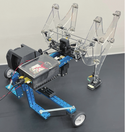
Fig. 2. Developed robot.
The GRF is an important mechanical element for gait control because it is an external force associated with walking, along with gravity and inertia. The CPG realizes stabilization and transition of motion in response to external inputs by means of stability points and bifurcation points intrinsic to the neural mechanism. Passive walking arbitrarily creates stable points inherent in the body’s dynamic system, including the environment, through body design, and realizes stable motion, but motion transitions are difficult to achieve.
Meanwhile, this study suggests a design theory that realizes motion transition as well as creating a stable point by body design. For bipedal walking, when the GRF transmitted to the legs is not equal when both legs are in the stance phase, internal forces are generated in the body, causing the animal to fall (Fig. 1(a)). In other words, the animal has a mechanism to equalize the GRF acting on both legs within the body, and this mechanism is assumed to generate a stable gait pattern without falling. Focusing on the mechanism for maintaining postural stability, we developed a robot equipped with a differential gear to achieve the equalization of the GRF 43. In studies that employ CPGs or sensory feedback, each leg is typically equipped with one or more actuators. Under such arrangements, variations in ground reaction forces and individual motor characteristics make it difficult to keep the applied torque strictly constant unless a complete electro-mechanical model of each motor is available. In our work, the differential gear ensures equal torque distribution, enabling us to investigate the problem with a considerably simpler robot than those used in previous research. Note that our research does not claim originality in the mere incorporation of a differential mechanism into a robot, while geared differential design allow to build an extremely minimal robot for studying rhythmic locomotion in multi-legged systems that lack any electronic control circuitry. Figs. 1(b)–(e) shows the relationship between the differential device to eliminate the internal rotational forces and the generation of a rhythmic motion in a leg-equipped robot.
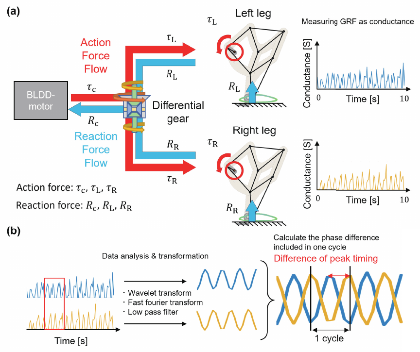
Fig. 3. Overview.
The red arrows represent the flow of force and torque until the input torque from the motor slips on the ground. Conversely, the blue arrows represent the reaction force or counter-torque that the legs receive from the ground. The shafts that power each leg are coupled by a motor and differential mechanism that can absorb each speed difference while achieving equal rotational force distribution.
The gait generated by the leg-equipped robot developed here was not reproducible and did not reach the point of motion stabilization. In addition, no theoretical analysis was conducted at all, and it is necessary to clarify the normative principles by attempting to formulate the phenomenon. This differential gear eliminates angular velocity differences and equalizes the driving force 44, and it is based on a device mainly used in automobiles. Experiments using the leg-equipped robot confirmed that the robot generates a stable rhythmic motion in response to the input torque.
Our robot allows only the difference in angular velocity (or angle) between the hind legs. Even with this simpler constraint, stability has been demonstrated through actual experiments, enabling rhythmic motion generation. In this regard, the experimental setup differs from those based on GRF for gait generation.
3. Methods
3.1. Scheme of Robot Experiments
We developed a leg-equipped robot (Fig. 2), conducted walking experiments, measured its behavior, and compared it with a mathematical model to explore the proposed rhythmic motion mechanism (Fig. 3). Walking experiments were conducted using the developed leg-equipped robot. The torque input from the motor is transmitted to the left and right legs via a differential gear (Fig. 3(a)). Owing to the geometrical structure of the legs, a swing phase and a stance phase appear with each rotation of the drive shaft. The GRF generated by the contact between the left and right toes and the ground is transmitted to the motor via the differential gear. The generated GRF was measured using a pressure-sensitive sensor, and the change in the resistance of the pressure-sensitive sensor was converted to conductance. The data measured as conductance contained considerable noise owing to the flapping of the foot. Here, wavelet transform, fast Fourier transform (FFT), and a low-pass filter were applied to reduce the noise (Fig. 3(b)). The time between the adjacent peaks of the obtained waveforms was one period. The difference between the peak timing of the left and right waveforms was calculated based on the waveform of the data obtained from the right leg, and the value obtained by multiplying the ratio of the time difference to one cycle by 2\(\pi\) was expressed as the phase difference between the legs.
3.2. Robot Design
Our robot has the following features. I) A differential gear was used to transmit the driving force from a single motor to the left and right legs equally. II) The Theo–Janssen mechanism was used for both legs. This allows the trajectory of the toes to be adjusted by setting the length of each link arbitrarily.
Our robot weighs 2.452 \(\mathrm{kg}\) and has a degree of freedom in the yaw direction, in addition to the rotational axes of both legs. It is equipped with a mechanism that allows passive rotation in response to the movement of its legs. By providing degrees of freedom at the connection between the front wheels and the main body, the mechanism encourages the front wheels and the main body to move independently, preventing the friction of the front wheels from affecting the main body.
The robot is equipped with a single brushless DC motor. The motor was rated at 24 \(\mathrm{V}\) and operates at a maximum no-load speed of 320 \(\mathrm{rpm}\) and a maximum continuous torque of 1.2 \(\mathrm{Nm}\). The motor controls the input torque by controlling voltage via pulse width modulation (PWM) in the range of 0\(\mathrm{\%}\)–100\(\mathrm{\%}\) using controller area network (CAN) communication with 1 Mbps speed. The current flow through the motor and the rotation speed can be obtained as feedback information. The motor has back-drivability, which means that it can receive the reaction force from the ground as a single force input (Figs. 1(b)–(e)).
Pressure-sensitive sensors were attached to the robot’s soles to measure the GRF. The phase difference was obtained from the time variation of the measured GRF to determine whether the left or right leg was in a swing or stance phase.
3.3. Differential Gear
Differential gears are mechanical parts installed in vehicles such as automobiles and are useful when a speed difference occurs at the end of left and right shafts, such as when turning. As a vehicle turns, a speed difference arises between the inner and outer wheels. The differential gear absorbs this speed difference while simultaneously transmitting torque equally from the drive source to both the inner and outer wheels, thereby facilitating smooth driving 44.
Differential gears have various types, including shaft-driven and belt-driven types 45. Shaft-driven gears are used in automobiles because of their superior power transmission efficiency and strength. The belt-driven type is used in radio-controlled vehicles because of its simple structure, ability to transmit power between distant shafts, and superior quietness. Therefore, a belt-driven differential gear is used in this study.
The belt-driven differential gear comprises mechanical elements, such as a differential pulley integrated with the differential case, side gears, pinion gears, and cross shaft. The pinion gears mesh with the side gears on both sides, allowing them to rotate on their own axes around the cross shaft and revolve around the axes of the side gears. The gear ratio between the pinion gear and the side gear used in this study is \(5:9\). Moreover, to minimize damping effects, a low-friction strategy is pursued by avoiding the injection of oil into the gear case. Torque is transmitted from the timing belt to the differential pulley, the differential pulley and differential case rotate as a single unit, and torque is transmitted to side gears by the pinion gear’s revolution. When the angular velocities of the left- and right-side gears, \({\omega_{\rm{L}}}\) and \({\omega_{\rm{R}}}\), are different and a differential drive is performed (Fig. 4), the following equation holds:
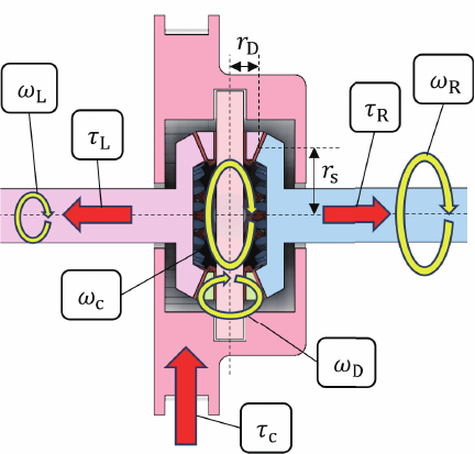
Fig. 4. Definitions of variables and physical parameters used in the differential principle.
3.4. Phase Analysis
We attached a pressure-sensitive sensor to the soles of bothblegs without performing calibration to acquire leg phase data and measured the leg phase from the timing of the leg ground contact (Fig. 3(a)). The pressure-sensitive range was 0.3–9.8 \(\mathrm{N}\), the pressure-sensitive area was \(39.6~\mathrm{mm} \times 39.6~\mathrm{mm}\), and the basic resistance was 20 M\(\Omega\) or higher. The resistance of the pressure-sensitive sensor was obtained using a voltage divider circuit, and the pressure-sensitive pressure value was output as the conductance \(G\) [S].
Since the conductance data obtained using this approach contain a lot of noise (Fig. 5), a wavelet transform was first performed (see Appendix A.2). This allows the waveforms that involve multiple peaks due to noise to be identified as a single peak. Furthermore, FFT analysis was performed to visualize the frequency domain of the leg rotation axis and the high-frequency domain due to noise (see Appendix A.3), and a low-pass filter was used to remove the high-frequency domain, including the noise (see Appendix A.1).
Using the waveforms of the left and right leg data with the reduced noise, the phase difference was calculated from the ratio of the time difference in the peak timing of the waveforms included in one cycle (see Appendix A.4).
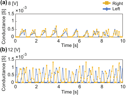
Fig. 5. Experimental data collected during locomotion.
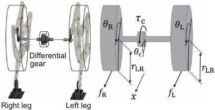
Fig. 6. Mathematical approximation model.
3.5. Mathematical Model
In this section, rather than directly analyzing periodic motions, we focus on identifying bifurcation phenomena that arise as system parameters vary and on characterizing the types of these bifurcations. A simple mechanical model was developed for the robot (Fig. 6). Here, only the differential gear necessary for the system to operate, the left and right legs, and the axes necessary for the transmission of the driving force were retained. The left and right legs were cylinders (hereafter referred to as wheels) to avoid complications in the calculations, and various characters were defined for the differential gear and wheels \(\rm{L}\) and \(\rm{R}\) (Fig. 6). The subscripts \(\rm{c}\), \(\rm{L}\), and \(\rm{R}\) denote the differential gear, left wheel, and right wheel, respectively. The subscript \(\rm{LR}\) represents a common term. Additionally, Table 1 summarizes the various parameters and variables defined in this study.
The stability of walking motion is often formulated as a hybrid dynamical system. However, once such a formulation is adopted, conventional analytical methods developed for continuous functions can no longer be directly applied, making the analysis extremely difficult. Therefore, in this study, we intentionally minimized mathematical rigor and focused on whether bifurcation phenomena could emerge, which constitutes the main feature of our theoretical analysis. In gait stability analysis, Poincaré maps are commonly used to evaluate stability within a single gait cycle. From the perspective of gait pattern formation, however, it can also be valuable to investigate the continuous phase relationship between the legs rather than focusing solely on one cycle. We also aimed to include the non-differentiable transition points between the stance and swing phases in the analysis. To achieve this, we extracted only the simplest periodic component, which can be regarded as the first term of a Fourier series expansion, and approximated it as a differentiable continuous function. This approach enabled us to derive and analyze a self-consistent equation of motion46,47. This approximation was determined from the anteroposterior GRF \(F_{y}\) shown in Fig. 7, which was measured at the sole of the foot during human walking. The frictional force acting on the left and right wheels is defined by the following continuous function:
Table 1. Summary of parameters.

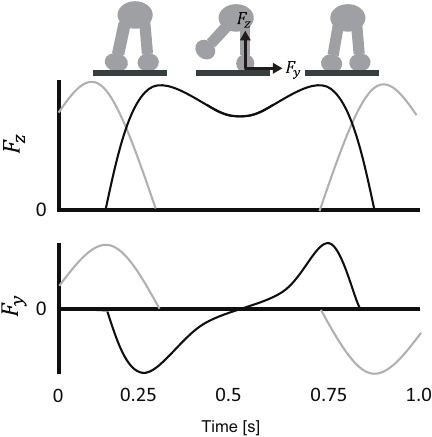
Fig. 7. Examples of ground reaction forces during walking. (\(F_{z}\) represents the vertical GRFs, while \(F_{y}\) represents the anteroposterior ground reaction forces. This figure was drawn with reference to 48,49,50).
The difference between the rotation angles of the left and right wheels, \(\theta_{\rm{L}}\) and \(\theta_{\rm{R}}\), is newly defined as the phase difference \(\phi\).
In our mathematical model, the equation of motion for the robot’s rhythmic motion is described by the equation of state, described as follows:
4. Results
4.1. Rhythm Generation
The developed robot was used in a walking experiment on a treadmill. Because the hardware design made it impossible to fix the initial conditions, we randomly assigned the initial phase difference by hand for all experiments in this study. This is because the initial posture and position of the robot are not able to explicitly predefined. First, the differential gear attached to the robot allows the shaft angles—and hence angular velocities—to transmit torque to both legs to vary according to Eq. (2). Second, owing to the back-drivability of the single brushless motor that serves as the sole power source, reverse torques can further alter these angles. Consequently, the robot always begins from a fully relaxed, load-free state; the front wheels may spin freely, and the initial posture is determined only by the robot’s own weight as it settles into static balance. In the walking experiment, the output torque \(\tau_{\rm{c}}\) of the motor was adjusted by arbitrarily changing the voltage value, which is the only parameter. When the load applied to the motor is not constant, the motor torque cannot remain fixed because the current fluctuates. Therefore, we adopt the voltage value as the variable so that the equilibrium state is uniquely defined. This allows the robot’s moving speed to vary with the voltage. We generally kept the treadmill stationary; however, when the robot’s locomotion speed became high, we operated it at a constant speed to prevent the robot from falling. The experiments were conducted 10 times for each voltage, from 7 \(\mathrm{V}\) to 15 \(\mathrm{V}\) in 0.5 \(\mathrm{V}\) increments, and the phase difference was quantitatively obtained.
Stable walking was observed at 12 \(\mathrm{V}\) as the voltage to the motor changed (Fig. 8(a)). Conversely, at 8 \(\mathrm{V}\), the phase difference showed a walk close to zero, resulting in difference from the behavior at 12 \(\mathrm{V}\). In addition, the measured raw data show different grounding timings (Fig. 5), which is considered to be a result of bifurcation in the dynamics consisting of the robot and the ground, with input torque as the bifurcation parameter.
These hardware experiments demonstrated that walking gait patterns can be generated without using control laws, such as the CPG, owing to spontaneous gait generation that takes advantage of environmental characteristics and body structure, as in the case of a passive walking robot. This walking can regulate gait generation via a single control input, with only one area where it is generated by increasing or decreasing the input torque from the motor under adjustable control and one area where it is not (disorderly or different gait is generated).
When the driving force from the motor was transmitted via a single shaft, the left and right legs maintained their initial phase difference, and no pattern was generated. Alternatively, in the case of the differential gear used in this study, the phase difference can change from moment to moment because the mechanism can tolerate changes in the phase of the left and right legs. In fact, in the experimental results, we obtained a region where the phase difference was not constant at an input value of 11.5 \(\mathrm{V}\). However, at 12 \(\mathrm{V}\), the robot continued to walk with a phase difference of \(\pi\), suggesting the existence of an attractor for a stable rhythmic motion.
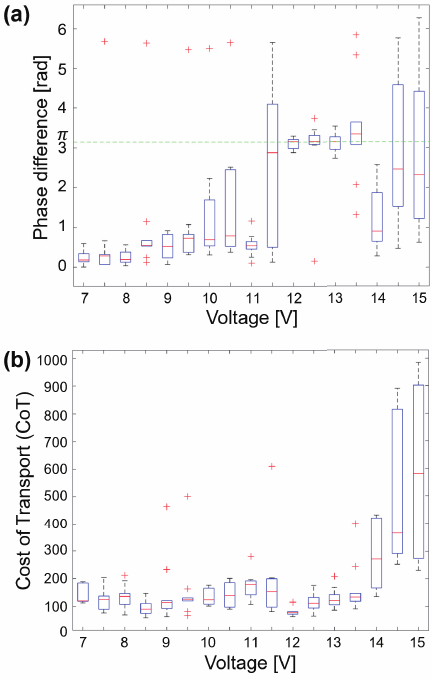
Fig. 8. The phase difference and CoT respond to variations in the driving force applied to the motor.
4.2. Energy Efficiency
To calculate the energy efficiency, we measured the distance traveled by the robot and the current value for each constant voltage value during a measurement time of 10 \(\mathrm{s}\). This allows us to calculate cost of transport (CoT) 51,52, which is expressed by the following equation:
4.3. Mathematical Analysis
Mathematical analysis was performed to gain a more detailed understanding of motion stability and when walking is generated.
Here, the fixed points of the equation of state are described as follows:
The Jacobi matrices and their eigenvalues were calculated around each fixed point to determine the stability of the fixed points (see Appendix C.1). The eigenequations of each Jacobi matrix are described as follows:
The fixed point \(\boldsymbol{x}_{1}^{*}\) is unstable because it has eigenvalues with positive real parts. From the coefficients \(f_{\mathbf{A}_{3}}(\xi_{3})\) and \(f_{\mathbf{A}_{4}}(\xi_{4})\), Hurwitz’s stable discriminant method shows that the fixed points \(\boldsymbol{x}_{3}^{*}\) and \(\boldsymbol{x}_{4}^{*}\) are also always unstable. On the other hand, for \(\boldsymbol{x}_{2}^{*}\), the stability discriminant is determined by the positive and negative values of the real parts of the eigenvalues, where \(\cos(\sin^{-1}({\tau_{\rm{c}}}/({2Fr_{\rm{LR}}}))) = \sqrt{1 - ({\tau_{\rm{c}}}/({2Fr_{\rm{LR}}}))^{2}}\).
Assuming \(i(\xi_{2}) = 0,\ j(\xi_{2})=0\) based on Eq. (14), the following four eigenvalues are obtained:
The eigenvectors corresponding to each eigenvalue are described as follows:
These eigenvectors represent the direction of convergence and divergence of the fixed point \(\boldsymbol{x}_{2}^{*}\) on the phase diagram, and the magnitude of the eigenvalue is the system gain that indicates the degree of its decay or amplification. Thus, we obtain \(\mathrm{Re}(\xi_{22}) < 0\) and \(\mathrm{Re}(\xi_{24}) < 0\) for the real part of each eigenvalue, whereas \(\mathrm{Re}(\xi_{21})\) and \(\mathrm{Re}(\xi_{23})\) are positive or negative depending on the value of \(\tau_{\rm{c}}\). Therefore, the real part of the eigenvalues \(\mathrm{Re}(\xi_{21})\), where \(c_{\rm{LR}} = I_{\rm{LR}} = F = r_{\rm{LR}} = 1,\) for the input torque \(\tau_{\rm{c}}\), was plotted using numerical analysis (Fig. 9(a)). The Jacobian matrix \(\rm{\bf{A}}_{1}\) is a block diagonal matrix, and the stability with respect to the phase difference is determined by \(\mathrm{Re}(\xi_{21})\) and \(\mathrm{Re}(\xi_{22})\). Therefore, only the results for \(\mathrm{Re}(\xi_{21})\) are shown here, but \(\mathrm{Re}(\xi_{23})\) exhibits similar properties to \(\mathrm{Re}(\xi_{21})\). As a result, when the input torque \(\tau_{\rm{c}}\) is \(0\leq \tau_{\rm{c}}<2\), the fixed point \(\boldsymbol{x}_{2}^{*}\) is stable, and the phase difference is 0. The red line represents the mathematically calculated bifurcation point. Therefore, it shows a stable motion with a phase difference of 0. This result is consistent with the motion observed in the walking experiment for the voltage range of 7–11 \(\mathrm{V}\). If the value of \(\tau_{\rm{c}}\) is \(2 < \tau_{\rm{c}}\), the real parts of the eigenvalues are negative, indicating destabilization.
In addition, the results of the eigenvalue analysis of the nondimensionalized mathematical model are plotted with \(\bar{\tau}_{\rm{c}}\) on the horizontal axis and \(\bar{F}\) on the vertical axis (Fig. 9(b)). Assuming the real part of the eigenvalues to be 0 (that is, at the bifurcation boundary indicated by the red line), we obtain \(\bar{\tau}_{\rm{c}}/\bar{F} = 0,2\). \(\bar{\tau}_{\rm{c}}/\bar{F} = 2\) indicates that at the moment \(\bar{\tau}_{\rm{c}}/\bar{F} = 2\), the system diverges from a stable state (zero phase difference) to an unstable state. However, \(\bar{\tau}_{\rm{c}}/\bar{F} = 0\) indicates that \(\bar{\tau}_{\rm{c}} = 0\), and no input torque is applied; therefore, it was not included in the analysis.
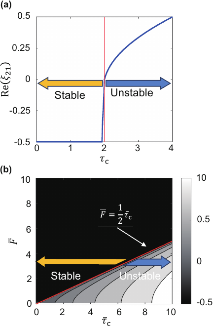
Fig. 9. Visualization of stability changes in response to input torque.
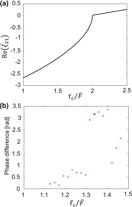
Fig. 10. Experimental results versus mathematical analysis in the vicinity of rhythm generation.
4.4. Comparison of the Experimental and Mathematical Results
The results of the mathematical analysis were compared with those of the actual experiment conducted using nondimensionalization. To compare the results with continuous mathematical values, it is desirable to use experimental data with more subdivided input voltage values. Therefore, the median phase difference at each voltage, obtained from walking experiments conducted 10 times per voltage, was used to compare with the mathematical analysis. The values of the real part of the eigenvalues (black line) and the phase difference (green star) versus the ratio of the dimensionless quantity \(\bar{\tau}_{\rm{c}}\) and \(\bar{F}\) are plotted in Fig. 10. The black line represents the predicted change in stability based on the non-dimensionalized Eq. (18). The red square represents the data point at 12 \(\mathrm{V}\) in the actual machine experiments, where a phase difference of \(\pi\) was found to be the most stable. Comparative examination of Figs. 10(a) and (b) demonstrates that the qualitative state transitions associated with bifurcation exhibit equivalent characteristics.
4.5. Visualization of Frequency Distribution
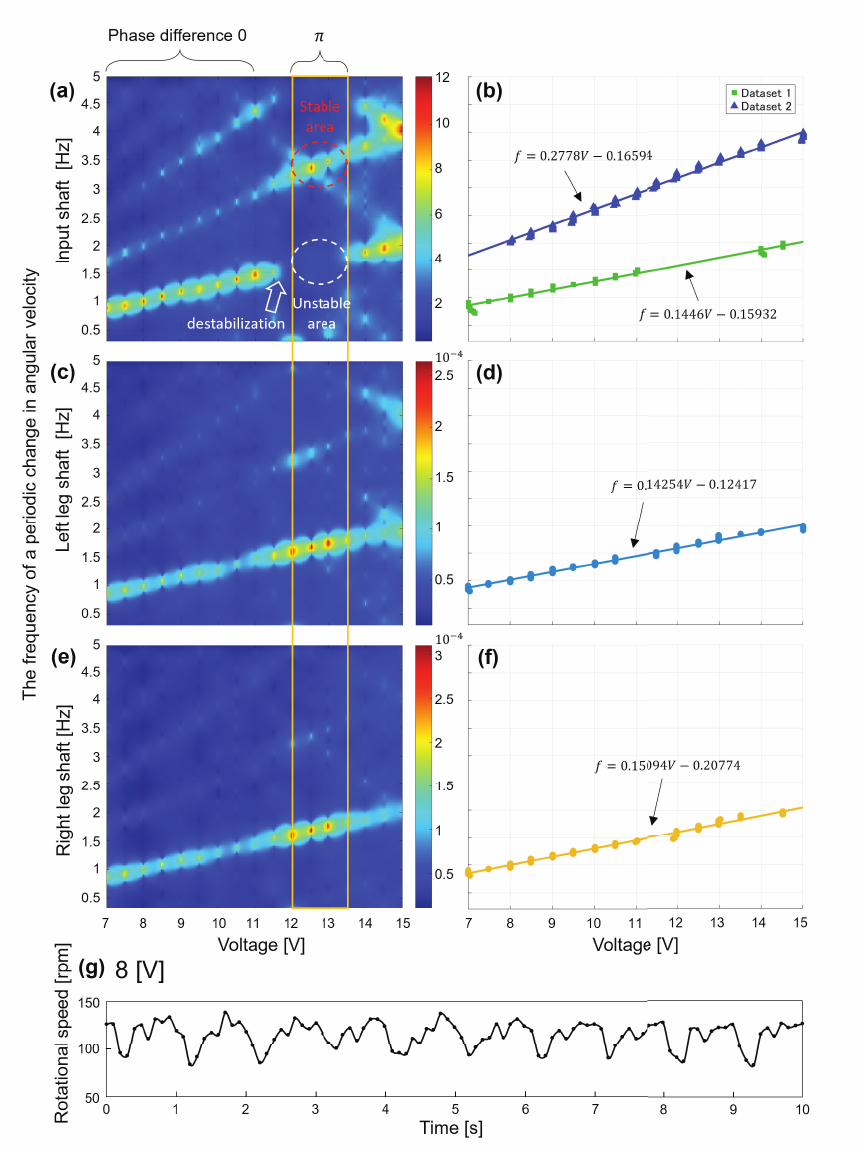
Fig. 11. The frequency of angular velocities around differential gear shafts.
We visualized the time-series data of the motor’s angular velocity for each voltage value obtained in Section 4.1, specifically the angular velocity of the differential gear’s input shaft and the GRFs data of both legs. The heatmap in Fig. 11 displays frequency on the vertical axis and voltage values on the horizontal axis, with color intensity representing the amplitude magnitude obtained from the FFT. However, amplitudes below 0.2 \(\mathrm{Hz}\) exhibit significant noise and were therefore excluded beforehand. Additionally, Figs. 11(b), (d), and (f) present the lines obtained by applying the least squares method to data sampled from Figs. 11(a), (c), and (e), respectively. These sampled data represent the maximum amplitude for each voltage value, and the sampling ranges differ for each corresponding figure. The heatmap was created based on a \(200 \times 200\) grid, resulting in approximately 0.04 \(\mathrm{V}\) increments. In Fig. 11(a), two datasets were created, defined as:
Figure 11(a) shows that the frequency of angular velocity change increases discretely at a voltage value of approximately 12–13.5 \(\mathrm{V}\). Because the motor’s angular velocity varies such that it oscillates periodically (Fig. 11(g)), it can be expressed by the following equation.
Focusing on the amplitude ratio, we derive:
5. Discussion and Conclusion
Instead of using the previously proposed gait generation mechanism, we observed that rhythm generation occurs spontaneously owing to the structure of the leg-equipped robot. These results are different from those of conventional gait generation modes (e.g., CPG or passive walking) and may provide an innovative approach for realizing robot locomotion.
In the proposed robot with a differential gear, equal torque distribution is shown to contribute to the realization of a rhythmic gait. Interactions of robots with their environments have been shown to play a significant role in realizing animal-like gait patterns; however, few concrete principles have been developed. The constraints imposed by the differential gear are expressed as a simple mathematical equation and are expected to be effective in the mathematical modeling of complex interactions between the body and the environment. Our simple mechanical model comprises a differential gear and two wheels, and the discrete ground contact timing of the legs is represented by a continuous function.
Although the stability analysis failed to find a stable fixed point for \(2<\tau_{\rm{c}}\), the results of the actual experiment suggest the existence of a stable fixed point where the phase difference is \(\pi\). One possible reason for the difference between the stable region observed in the experiment and the stable fixed point calculated by the mathematical model is that the friction force is approximated by a periodic function in the mathematical model (Eq. (4)). Eq. (4) approximates the vertical ground-reaction force \(F_{y}\) shown in Fig. 7; however, during actual walking there are intervals in which \(F_{y}\) becomes zero, and Eq. (4) cannot adequately capture this portion of the waveform. The interval where \(F_{y}=0\) corresponds to the swing phase of gait, whereas in Eq. (4) this condition is reduced to instantaneous events only at \(\theta_{i}=0\) and \(\theta_{i}=\pi\). We consider that a stable fixed point at a phase difference of \(\pi\) is not observed because energy is dissipated by friction in every state other than \(\theta_{i}=0, \pi\). The derivation of a self-consistent equation of motion using periodic functions is effective for analyzing gait behavior over multiple cycles, and thus differs from stability analyses based on the Poincaré map, which focus only on a single gait cycle. We consider this approach to be one of the effective means for analyzing not only the stabilization of gait patterns but also their generation. In fact, at low torque, the phase difference is 0, which is the same result for both the actual machine and the mathematical model, so it is considered to be a reasonable approximation to some extent. On the other hand, at high torque, the phase difference was stable at \(\pi\) in the actual machine, but in the mathematical model, after destabilization, there was no stable fixed point. This difference indicates that the nonlinearity inherent in the yield transition was not well captured by the simple sinusoidal approximation.
The physical meaning of \(\bar{\tau}_{\rm{c}}/\bar{F} = 2\), which is the result of bifurcation analysis using the mathematical model, is that a single input \(\bar{\tau}_{\rm{c}}\) is balanced by two wheels, or \(\bar{F}\), the load received by both legs in the leg-equipped robot. This relationship suggests that an imbalance between the driving force and the load from the external environment is essential for spontaneous rhythm generation. If the input torque is constant and the load from the environment varies, the motion is determined by the load. Thus, our robot can spontaneously generate rhythmic motion as an adaptive response to the load from the environment.
The reason why the angular acceleration doubled within a specific voltage range in Section 4.5 can be explained from an energetic perspective. A general energy-related equation can be expressed as:
Based on the model that requires GRF equalization for stable rhythm generation, we devised a leg-equipped robot and a mechanical model to satisfy this constraint. Consequently, we confirmed stable rhythm generation for the leg-equipped robot and found new conditions for spontaneous rhythmic behavior in the mathematical model. Interesting findings regarding the balance between leg driving forces and the GRF in the design of BirdBot were reported 53. The instability was introduced by configuring an underbalanced pulley in which the joint radii of the legs were smaller than those in the moment-balanced case. In other words, an imbalance between the external load torque and the tendon driving force (extension torque) from inside the body was arbitrarily created. This allowed for quicker joint flexion compared to that of a joint with a balanced radius. In contrast, our leg robot creates an imbalance by increasing the input torque.
Similarly, a study has been reported 54 that achieves gait pattern generation through interactions between the body and the environment without relying on explicit control. Interestingly, the researchers constructed a drive system by connecting tubes so that, like a differential gear, it functions with one input and two outputs. By varying the pneumatic pressure supplied to the tube, they observed changes in the robot’s behavior. Such motion generation based on the mechanical interaction between the robot and its surroundings is an excellent example of naturally emergent locomotion without control, and it is expected to spur further developments in this field.
To sum up, we found that the balance between the load transmitted to the leg and the driving force can be one of the important factors of rhythmic motion. The GRF equalization mechanism stabilizes the motion during locomotion and thus generates rhythmic behavior, which could be a new criterion for motion generation. This finding highlights the significant role of incorporating inputs from the external environment in the generation of locomotion such as rhythmic walking. Furthermore, this study suggests that accommodating internal forces could serve as an effective approach to achieving stable walking behavior. The differential gear mechanism employed in this study simply distributes torque evenly between the two legs. This means that, during the stance phase, when both legs are in contact with the ground, the mechanism itself inherently minimizes energy loss. This study does not claim that such a mechanism exists in animal bodies. However, the results indicate that dissipating internal forces could provide a novel hardware-based means for achieving stable locomotion, which has not been explored in previous studies.
In general, GRFs are crucial mechanical feedback obtained through the interaction between the body and the environment during locomotion. In CPG models and sensory feedback systems, sensory inputs corresponding to GRFs are used to adjust oscillator phases, thereby enabling stable rhythmic walking. In contrast, this study demonstrated a process in which rhythmic patterns spontaneously emerge through the mechanical constraints of the body. In this process, the GRFs observed in the developed robot are not merely feedback signals but can be regarded as input energy that drives the formation of internal order within the body.
The energetic considerations of this study suggest that rhythmic motion is generated by the energy balance pertaining to the work done by energy inflow/outflow and physical rhythmic motion, rather than by the generation of motion through conventional control of dynamics. These are expected to lead to the design of existing gait control systems based on energy inflow and outflow. The robot developed in this study is a very simple mobile robot, i.e., it is realized by simply distributing the driving force of one degree of freedom equally. We have shown that this developed robot can generate rhythm with energy inflow/outflow, provided that it has the appropriate body structure. We believe that our findings, which suggest that the mechanism that maintains the stability of the locomotion posture contributes to the realization of rhythmic locomotion, and that this is what allows for a stable gait, provide another perspective in biology.
Appendix A. Analysis of the GRF
A.1. Waveform After Low-Pass Filter
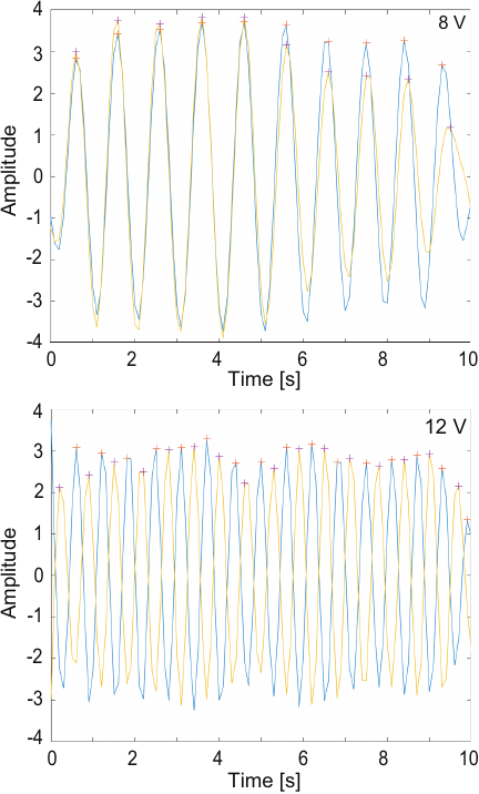
Fig. 12. Motions data extraction by waveform after the low-pass filter.
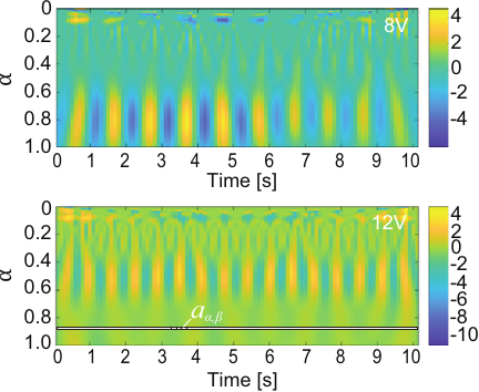
Fig. 13. Definition of the phase in walking obtained by wavelet transforms.
The experimental data are shown when the input voltage to the motor was 8 V and 12 V. In each Fig. 12, the blue line represents the experimental data for the left leg and the yellow line, for the right leg. The frequency at which the one-sided spectrum of the FFT reached its maximum was considered as the ground motion from the swing leg to the support leg, and the higher frequency components were removed.
A.2. Wavelet Transform
Experimental data are shown for motor input torques of 8 \(\mathrm{V}\) and 12 \(\mathrm{V}\). Fig. 13 shows the data of the right leg. Since the highlighted areas are the main frequency components of the acquired data, they are extracted and used for the phase difference analysis. The Morlet function expressed as a wavelet was used: \(mw(x) = {\exp}^{-({x^{2}}/{2})}\cos5x\), where \(x = {(t-\beta)}/{\alpha}\). \(t\): time of experimental data, \(\alpha\) and \(\beta\): parameters of the wavelet. Specifically, in this study, \(\alpha\) ranges from 0.000 to 1.000 and \(\beta\) ranges from 0.1 to 10.0. Furthermore, the data to be extracted was obtained by selecting \(\alpha\) that satisfies the following:
A.3. Fast Fourier Transform (FFT)
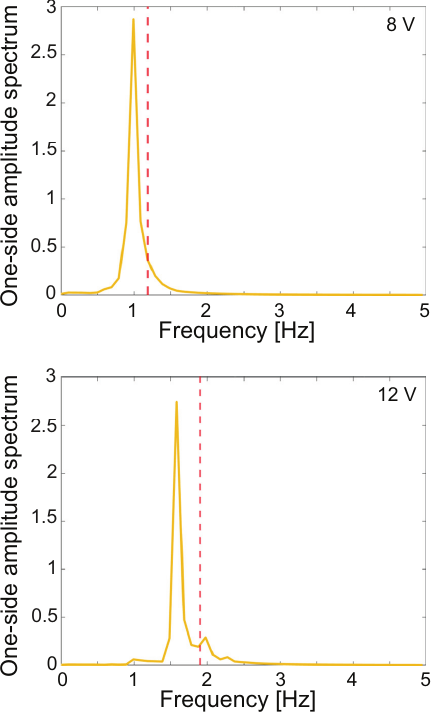
Fig. 14. Extractions of motion frequency by fast Fourier transform (FFT).
Experimental data are shown for motor input torques of 8 \(\mathrm{V}\) and 12 \(\mathrm{V}\) (Fig. 14). In the data extracted by the wavelet transform, a larger input voltage value results in increased noise. The main frequencies are visualized using toolbox on MATLAB fft function to reduce noise. The sampling frequency for the FFT was set to 10 \(\mathrm{Hz}\) because the experimental data were measured every 0.1 seconds. The red dashed line shows the frequency when the correction value is multiplied by 1.2 times the frequency when the one-sided spectrum is at its maximum. Note that these cutoff frequencies can take different values in each data.
A.4. Calculation of the Phase Difference
The phase difference was calculated by focusing only on the maximum value (“\(+\)" in Fig. 12) of each waveform. First, the average period \(T_{\rm{L}\_\mathit{ave}}\) and \(T_{\rm{R}\_\mathit{ave}}\) of each waveform obtained is calculated by the following equation.
From the above, the phase difference is obtained from the ratio of the average time difference of each maximum value to the average of the average period of the waveforms obtained from the left and right legs.
The above equation calculates the phase difference by multiplying the ratio of the phase difference in one period by the phase of one period, \(2\pi\).
Table 2. Weight distribution at each support point for different components.

Appendix B. Effect of CoG Position on Motion Stability
One important contribution to stabilization by the wheels is weight distribution at each support point. Although the robot cannot stand up autonomously, additional experiments have shown that the position of the CoG affects rhythm generation. Experimental results indicate that leg loading is essential for stable rhythm generation.
To investigate the relationship between load on the legs and rhythm generation, additional walking experiments were conducted at 12 V, where the robot exhibited the most stable walking. The weights attached to the robot were positioned in three different locations: front, center, and rear. The results of weight measurements corresponding to each weight position, taken at four points including the front wheels and the legs, are shown in Table 2. However, slight variations in the measurements may occur due to the cables connected to the Arduino. Each configuration was tested in 10 trials. Notably, the rear position corresponds to the same location used in walking experiments in Section 4.1. Using the same method as described in Section 3.4, the phase differences were calculated and summarized in Fig. 15. The result indicates that as the CoG shifts closer to the front (towards the front wheels), rhythm generation stability decreases, eventually leading to the inability to generate walking. This suggests that an appropriate load on the legs is essential for rhythm generation.
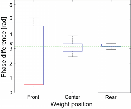
Fig. 15. Motion stability based on CoG position.
Appendix C. Details of Mathematical Analysis
C.1. Jacobi Matrix
The linearization of Eq. (7) is shown below using the Jacobi matrix obtained around fixed point \(\boldsymbol{x}^{*} = [\dot{\phi}^{*}, \phi^{*},\dot{\theta}_{\rm{c}}^{*}, \theta_{\rm{c}}^{*}]^{\rm{T}}\):
C.2. Nondimensionalization
Equation (7) is nondimensionalized with representative scales as \({M} = I_{\textrm{LR}}/r_{\textrm{LR}}^{2}, {L} = r_{\textrm{LR}}\), and \({T} = I_{\textrm{LR}}/c_{\textrm{LR}}\). Table 3 shows the parameters obtained upon nondimensionalization. After the nondimensionalization of Eq. (7), the following equation is obtained:
Table 3. Nondimensionalization of parameters.

Acknowledgments
The authors would like to thank K. Isomura for his assistance in the construction of the robot. This work was partly supported by JSPS KAKENHI Grant Numbers JP23H03480, JP25KJ2193.
- [1] R. M. Alexander, “The gaits of bipedal and quadrupedal animals,” Int. J. Robot. Res., Vol.3, No.2, pp. 49-59, 1984. https://doi.org/10.1177/027836498400300205
- [2] R. M. Alexander, “Bipedal animals, and their differences from humans,” J. Anat., Vol.204, No.5, pp. 321-330, 2004. https://doi.org/10.1111/j.0021-8782.2004.00289.x
- [3] P. Fihl and T. B. Moeslund, “Classification of gait types based on the duty-factor,” IEEE Conf. on Advanced Video and Signal Based Surveillance, 2007. https://doi.org/10.1109/AVSS.2007.4425330
- [4] A. E. Minetti, “The biomechanics of skipping gaits: A third locomotion paradigm?,” Proc. Biol. Sci., Vol.265, No.1402, pp. 1227-1235, 1998. https://doi.org/10.1098/rspb.1998.0424
- [5] D. M. Wilson, “Insect walking,” Annu. Rev. Entomol., Vol.11, pp. 103-122, 1966. https://doi.org/10.1146/annurev.en.11.010166.000535
- [6] K. Naniwa et al., “Novel Method for Analyzing Flexible Locomotion Patterns of Animals by Using Polar Histogram,” J. Robot. Mechatron., Vol.32, No.4, pp. 812-821, 2020. https://doi.org/10.20965/jrm.2020.p0812
- [7] G. Hayes and R. M. Alexander, “The hopping gaits of crows (Corvidae) and other bipeds,” J. Zool., Vol.200, No.2, pp. 205-213, 1983. https://doi.org/10.1111/j.1469-7998.1983.tb05784.x
- [8] D. F. Hoyt and C. R. Taylor, “Gait and the energetics of locomotion in horses,” Nature, Vol.292, No.5820, pp. 239-240, 1981. https://doi.org/10.1038/292239a0
- [9] T. J. Dawson and C. R. Taylor, “Energetic cost of locomotion in kangaroos,” Nature, Vol.246, No.5431, pp. 313-314, 1973. https://doi.org/10.1038/246313a0
- [10] Z. Wang et al., “Optimization design and performance analysis of a bionic knee joint based on the geared five-bar mechanism,” Bioengineering (Basel), Vol.10, No.5, Article No.582, 2023. https://doi.org/10.3390/bioengineering10050582
- [11] A. Sayyad, B. Seth, and P. Seshu, “Single-legged hopping robotics research—A review,” Robotica, Vol.25, No.5, pp. 587-613, 2007. https://doi.org/10.1017/S0263574707003487
- [12] G. Heppner et al., “LAUROPE – Six legged walking robot for planetary exploration participating in the SPACEBOT cup,” WS Adv. Space Technol. Robot. Autom., Vol.2, No.13, pp. 69-76, 2015.
- [13] T. Kinugasa and Y. Sugimoto, “Dynamically and Biologically Inspired Legged Locomotion: A Review,” J. Robot. Mechatron., Vol.29, No.3, pp. 456-470, 2017. https://doi.org/10.20965/jrm.2017.p0456
- [14] G. Taga, Y. Yamaguchi, and H. Shimizu, “Self-organized control of bipedal locomotion by neural oscillators in unpredictable environment,” Biol. Cybern., Vol.65, pp. 147-159, 1991. https://doi.org/10.1007/BF00198086
- [15] E. Marder and D. Bucher, “Central pattern generators and the control of rhythmic movements,” Curr. Biol., Vol.11, No.23, pp. R986-R996, 2001. https://doi.org/10.1016/s0960-9822(01)00581-4
- [16] J. J. Collins and S. A. Richmond, “Hard-wired central pattern generators for quadrupedal locomotion,” Biol. Cybern., Vol.71, pp. 375-385, 1994. https://doi.org/10.1007/BF00198915
- [17] Y. Fukuoka, Y. Habu, and T. Fukui, “A simple rule for quadrupedal gait generation determined by leg loading feedback: A modeling study,” Sci. Rep., Vol.5, Article No.8169, 2015. https://doi.org/10.1038/srep08169
- [18] A. J. Ijspeert, “Central pattern generators for locomotion control in animals and robots: A review,” Neural Netw., Vol.21, No.4, pp. 642-653, 2008. https://doi.org/10.1016/j.neunet.2008.03.014
- [19] D. Owaki and A. Ishiguro, “A quadruped robot exhibiting spontaneous gait transitions from walking to trotting to galloping,” Sci. Rep., Vol.7, No.1, Article No.277, 2017. https://doi.org/10.1038/s41598-017-00348-9
- [20] T. Fukui, S. Matsukawa, Y. Habu, and Y. Fukuoka, “Gait transition from pacing by a quadrupedal simulated model and robot with phase modulation by vestibular feedback,” Robotics, Vol.11, No.1, Article No.3, 2022. https://doi.org/10.3390/robotics11010003
- [21] J. Humphreys et al., “Bio-inspired gait transitions for quadruped locomotion,” IEEE Robot. Autom. Lett., Vol.8, No.10, pp. 6131-6138, 2023. https://doi.org/10.1109/LRA.2023.3300249
- [22] C. P. Santos and V. Matos, “Gait transition and modulation in a quadruped robot: A brainstem-like modulation approach,” Robot. Auton. Syst., Vol.59, No.9, pp. 620-634, 2011. https://doi.org/10.1016/j.robot.2011.05.003
- [23] S. Grillner, “Locomotion in vertebrates: Central mechanisms and reflex interaction,” Physiol. Rev., Vol.55, No.2, pp. 247-304, 1975. https://doi.org/10.1152/physrev.1975.55.2.247
- [24] T. G. Brown, “The intrinsic factors in the act of progression in the mammal,” Proc. Biol. Sci., Vol.84, No.572, pp. 308-319, 1911. https://doi.org/10.1098/rspb.1911.0077
- [25] T. McGeer, “Passive dynamic walking,” Intern. J. Robot. Res., Vol.9, No.2, pp. 62-82, 1990. https://doi.org/10.1177/027836499000900206
- [26] T. McGeer, “Passive walking with knees,” IEEE Int. Conf. on Robotics and Automation, pp. 1640-1645, 1990. https://doi.org/10.1109/ROBOT.1990.126245
- [27] T. McGeer, “Principles of walking and running,” Adv. Comp. Environ. Physiol., pp. 113-139, 1992.
- [28] L. Li et al., “High-Frequency Vibration of Leg Masses for Improving Gait Stability of Compass Walking on Slippery Downhill,” J. Robot. Mechatron., Vol.31, No.4, pp. 621-628, 2019. https://doi.org/10.20965/jrm.2019.p0621
- [29] S. Collins et al., “Efficient bipedal robots based on passive-dynamic walkers,” Science, Vol.307, No.5712, pp. 1082-1085, 2005. https://doi.org/10.1126/science.1107799
- [30] M. W. Spong and F. Bullo, “Controlled symmetries and passive walking,” IEEE Trans. Autom. Control, Vol.50, No.7, pp. 1025-1031, 2005. https://doi.org/10.1109/TAC.2005.851449
- [31] O. Makarenkov, “Existence and stability of limit cycles in the model of a planar passive biped walking down a slope,” Proc. Math. Phys. Eng. Sci., Vol.476, No.2233, Article No.20190450, 2020. https://doi.org/10.1098/rspa.2019.0450
- [32] M. Garcia et al., “The simplest walking model: Stability, complexity, and scaling,” J. Biomech. Eng., Vol.120, No.2, pp. 281-288, 1998. https://doi.org/10.1115/1.2798313
- [33] S. Iqbal et al., “Bifurcations and chaos in passive dynamic walking: A review,” Robot. Auton. Syst., Vol.62, No.6, pp. 889-909, 2014. https://doi.org/10.1016/j.robot.2014.01.006
- [34] S. Aoi et al., “A stability-based mechanism for hysteresis in the walk–trot transition in quadruped locomotion,” J. R. Soc. Interface, Vol.10, No.81, Article No.20120908, 2013. https://doi.org/10.1098/rsif.2012.0908
- [35] S. H. Strogatz, “Nonlinear Dynamics and Chaos: With Applications to Physics, Biology, Chemistry, and Engineering,” pp. 44-79, CRC Press, 2000.
- [36] A. Goswami, B. Thuilot, and B. Espiau, “A study of the Passive Gait of a Compass-Like Biped Robot: Symmetry and Chaos,” Int. J. Robot. Res., Vol.17, No.12, pp. 1282-1301, 1998. https://doi.org/10.1177/027836499801701202
- [37] K. Osuka and K. Kirihara, “Motion analysis and experiment of passive walking robot QUARTET II,” J. of the Robotics Society of Japan, Vol.18, No.5, pp. 737-742, 2000 (in Japanese). https://doi.org/10.7210/jrsj.18.737
- [38] S. Aoi et al., “Advanced turning maneuver of a many-legged robot using pitchfork bifurcation,” IEEE Trans. Robot., Vol.38, No.5, pp. 3015-3026, 2022. https://doi.org/10.1109/TRO.2022.3158194
- [39] M. Okada and K. Iwano, “Human interface design for semi-autonomous control of leader-follower excavator based on variable admittance and stagnation/trajectory bifurcation of nonlinear dynamics,” Mech. Eng. J., Vol.8, No.6, Article No.21-00127, 2021. https://doi.org/10.1299/mej.21-00127
- [40] X. Chen et al., “Foot Shape-Dependent Resistive Force Model for Bipedal Walkers on Granular Terrains,” Int. Conf. on Robotics and Automation, pp. 13093-13099, 2024. https://doi.org/10.1109/ICRA57147.2024.10610190
- [41] N. Scianca et al., “MPC for Humanoid Gait Generation: Stability and Feasibility,” Trans. on Robotics, Vol.36, No.4, pp. 1171-1188, 2020. https://doi.org/10.1109/TRO.2019.2958483
- [42] C. Chevallereau et al., “Self-synchronization and Self-stabilization of 3D Bipedal Walking Gaits,” Robotics and Autonomous Systems, Vol.100, pp. 43-60, 2018. https://doi.org/10.1016/j.robot.2017.10.018
- [43] K. Isomura et al., “Full time two-leg drive bipedal robot: Analysis of gait pattern generations under constraints of reaction forces equality,” Int. Conf. on Advanced Mechatronics, pp. 86-87, 2021. https://doi.org/10.1299/jsmeicam.2021.7.GS6-4
- [44] C. Singh et al., “A Study on Vehicle Differential system,” Int. J. Sci. Res. Manag., Vol.2, No.11, pp. 1680-1683, 2014.
- [45] S. Shinde et al., “Review paper on design of types of mechanical differentials used in automobiles,” Int. Res. J. Modernization Eng. Technol. Sci., Vol.3, No.1, pp. 1023-1031, 2021.
- [46] D. R. Hartree, “The Wave Mechanics of an Atom with a Non-Coulomb Central Field. Part II. Some Results and Discussion,” Math. Proc. Camb. Phil. Soc., Vol.24, No.1, pp. 111-132, 1928. https://doi.org/10.1017/S0305004100011920
- [47] H. Li et al., “Elastic-viscoplastic self-consistent modeling for finite deformation of polycrystalline materials,” Mater. Sci. Eng. A, Vol.799, No.2, Article No.140325, 2021. https://doi.org/10.1016/j.msea.2020.140325
- [48] K. Masani, M. Kouzaki, and T. Fukunaga, “Variability of ground reaction forces during treadmill walking,” J. App. Physiol., Vol.92, No.5, pp. 1885-1890, 2002. https://doi.org/10.1152/japplphysiol.00969.2000
- [49] T. Kobayashi et al., “Ground reaction forces during double limb stances while walking in individuals with unilateral transfemoral amputation,” Front. Bioeng. Biotechnol., Vol.10, Article No.1041060, 2022. https://doi.org/10.3389/fbioe.2022.1041060
- [50] A. Karatsidis et al., “Estimation of Ground Reaction Forces and Moments during Gait Using Only Inertial Motion Capture,” Sensors, Vol.17, No.1, Article No.75, 2017. https://doi.org/10.3390/s17010075
- [51] G. Gabrielli and T. von Karman, “What price speed?,” Vol.63, No.1, pp. 188-200, 1951. https://doi.org/10.1111/j.1559-3584.1951.tb02891.x
- [52] V. A. Tucker, “The Energetic Cost of Moving About,” Am. Sci., Vol.63, No.4, pp. 413-419, 1975.
- [53] A. Badri-Spröwitz et al., “BirdBot achieves energy-efficient gait with minimal control using avian-inspired leg clutching,” Sci. Robot., Vol.7, No.64, Article No.eabg4055, 2022. https://doi.org/10.1126/scirobotics.abg4055
- [54] A. Comoretto et al., “Physical synchronization of soft self-oscillating limbs for fast and autonomous locomotion,” Science, Vol.388, No.6747, pp. 610-615, 2025. https://doi.org/10.1126/science.adr3661
This article is published under a Creative Commons Attribution-NoDerivatives 4.0 Internationa License.