Development Report:
Analysis and Visualization of Growth Factors in Agricultural Data Using Explainable AI with L1/L2 Regularization
Haruki Hisatsune and Keiji Kamei
Department of Production Systems, Graduate School of Engineering, Nishinippon Institute of Technology
1-11 Aratsu, Kanda, Miyako, Fukuoka 800-0394, Japan

In this study, we propose a sparse recurrent neural network model with regularization to identify the environmental factors contributing to strawberry growth evaluation. The learning data consisted of eight environmental variables, including carbon dioxide concentration and solar radiation, measured by observation devices in a greenhouse. The target data included shipment volume, quality, growth status, and the farmer’s intuitive evaluation. Data obtained during three periods between February and March 2025 were used in this study. Model training was performed using backpropagation through time with the mean squared error as the loss function. To induce sparsity, L1 and L2 regularization were applied, suppressing moderately influential weights and yielding a more interpretable model structure. Unlike conventional black-box models that rely on post-hoc explanation techniques, the proposed method constructs an intrinsically interpretable learning model in which the influence of each environmental variable is directly reflected in the learned network structure. Rather than improving prediction accuracy, this study aimed to clarify the dominant environmental factors through a transparent and structurally constrained learning framework. The results suggested that growth evaluation was influenced by the carbon dioxide concentration around observation device 1, atmospheric pressure measured across multiple devices, and other environmental variables. These findings demonstrate that important environmental factors in strawberry cultivation can be effectively visualized, supporting transparent AI-based analysis and practical decision-making in agricultural production.
Visualization of quality-related factors using XAI
1. Introduction
Global employment in agriculture has experienced a long-term decline. According to recent statistics from the Food and Agriculture Organization of the United Nations, the global workforce engaged in agriculture, forestry, and fishing decreased from approximately 40% in 2000 to approximately 26% in 2023 a. This worldwide decrease in agricultural labor highlights the growing demand for labor-saving and automated technologies to manage agricultural produce. This trend is particularly evident in Japan. The number of core agricultural workers decreased from 1.757 million in 2015 to 1.021 million in 2025 b, indicating a substantial reduction in the agricultural labor force. In addition, the number of new farmers declined from 65,000 in 2015 to 43,500 in 2023, despite support programs implemented by the Ministry of Agriculture, Forestry and Fisheries c. These trends have resulted in a serious shortage of successors, posing a major challenge to sustainable agricultural growth.
Agricultural automation technologies have been actively developed in recent years, with particular emphasis on harvesting systems such as those used in robotic harvesting and autonomous field operations 1,2,3,4. Market analyses indicate that the global harvesting robot market was valued at approximately USD 2.2 billion in 2024 and is projected to grow to approximately USD 6.9 billion by 2030 d, reflecting the rapid expansion of automation for labor-intensive agricultural tasks. Despite this progress, clear quantitative indicators for appropriately managing crop growth based on environmental conditions have not yet been established. Therefore, in this study, we analyzed the environmental factors that contribute to variations in cultivation status, shipment volume, and quality. By focusing on growth factors such as temperature and humidity, which can be measured in agricultural greenhouses, this approach enables the visualization and analysis of crop growth and environmental conditions. The results are expected to support new farmers in their decision-making and contribute to establishing practical indicators for automating the production of agricultural produce.
In this study, we focused on strawberry cultivation and employed a recurrent neural network (RNN) 5,6, which is suitable for learning and modeling time-series data, to examine the relationship between growth evaluation data obtained from a farmer and meteorological and related information. We applied structural learning 7,8,9, a method proposed by Ishikawa and known as sparse modeling, to construct a sparse RNN and estimate the factors contributing to strawberry growth. Sparse modeling forces unnecessary regression link weights to approach zero by introducing the L1 norm, which is the sum of the absolute values of the link weights and biases, as a regularization term in the error function. This ensures that only the skeletal links necessary for regression are retained. This property can be used to extract important growth factors from the connections between the input and hidden layers. Thus, it is considered an explainable artificial intelligence (XAI) method that allows visualization of the AI’s decision-making criteria. Note that the purpose of this study was not to predict growth but to identify important cultivation attributes related to growth assessment through data analysis and visualization based on the XAI model structure.
In our previous studies 10,11, we constructed sparse RNN models by applying L1 and selective L1 regularization, through which we determined the relationship between shipping volume and atmospheric pressure. However, when only L1 regularization was used, many parameters with moderate influence tended to remain. Consequently, the distinction between important and unnecessary attributes was unclear, which reduced the interpretability of the model. Therefore, in this study, we established a method that combines the L1 norm with the L2 norm derived from the hidden layer outputs based on the approach proposed by Ishikawa 12. This method suppresses the excessive retention of weights with moderate effects and creates a more stable sparse representation. It also enables a clearer visualization of the environmental factors that contribute to crop growth, that is, the cultivation attributes relevant to AI modeling, compared with previous methods.
During this study, a sudden decrease in growth assessment values was observed from late February to March 2025. This period is generally regarded as the peak strawberry season, when high quality is typically maintained. Therefore, it is likely that the decrease in the assessment was caused by environmental growth factors, making it an important subject of analysis. This study aimed to identify the causes of this fluctuation during the specified period using the method proposed by Ishikawa 12.
The main scientific contribution of this study is an intrinsically interpretable learning model based on L1/L2 regularization, which can be used to identify and visualize the environmental factors affecting strawberry cultivation. Unlike previous studies that mainly focused on improving prediction accuracy or relied on post-hoc explanations for black-box models, this study emphasized factor identification through the model structure itself.
2. Related Work and Originality
2.1. AI Applications in Agriculture
Recent studies have demonstrated that AI and machine learning can be widely applied in agriculture for tasks such as crop yield prediction, disease detection, and decision support. Several review papers have reported that supervised and deep learning models, including random forests, support vector machines, and neural networks, are effective for modeling agricultural production using meteorological, soil, and remote-sensing data 13,14,15. For example, crop yield prediction is one of the most intensively studied topics, for which environmental variables such as temperature, rainfall, soil moisture, and vegetation indices are commonly used as explanatory factors 15,16,17. In addition to yield prediction, AI-based image recognition has been actively studied for use in plant disease detection and phenotyping. Convolutional neural networks have achieved high accuracy in classifying crop diseases from leaf images, enabling early diagnosis and labor-saving management practices 18,19. These studies indicate that AI has the potential to replace or complement the visual inspection performed by experienced farmers. Related studies have also been published in the Journal of Robotics and Mechatronics. Fujinaga et al. proposed a tomato growth state map for automating crop monitoring and harvesting and demonstrated the importance of visualizing crop growth states in robotic agricultural systems 20. In addition, Kase et al. investigated efficient robot learning based on motor babbling, which is relevant to data-driven modeling for robotic and agricultural applications 21. More recently, smart agriculture and precision farming systems have been integrated with Internet of Things sensors using AI techniques to analyze environmental conditions in real time 22,23. Machine learning models have been shown to effectively utilize sensor-based temperature, humidity, and soil data to optimize cultivation strategies and yield management 24,25. Furthermore, large-scale surveys and reports have emphasized that AI-driven agricultural technologies play a crucial role in improving productivity and sustainability under climate change conditions 13,14.
While most of these studies focused on improving prediction accuracy or automating recognition tasks, they often relied on black-box models, whose internal decision-making processes are difficult to interpret. To address this limitation, XAI was introduced to provide post-hoc explanations for complex models. Representative methods include Shapley additive explanations (SHAP) and local interpretable model-agnostic explanations (LIME), which estimate the contributions of input variables to model outputs 26,27. These methods have been applied to agricultural datasets to analyze the influence of weather and soil factors on crop yield and disease classification 24,25. However, these approaches still depend on black-box predictors, and interpretability is achieved only after model training. Moreover, because these explanations are generated by additional AI-based models, the explanation process itself becomes another black box. Consequently, these methods merely stack black-box models rather than fundamentally resolving the issue of model transparency.
2.2. XAI for Crop Factor Identification
XAI has been applied in the agricultural domain to analyze the influence of environmental and soil factors on crop yield and quality. For example, SHAP-based explanations have been used to quantify the effects of temperature, rainfall, and soil conditions on wheat yield prediction models 24. Similarly, explainable deep learning approaches have been applied to plant disease classification and hyper-spectral crop analysis, providing variable-level explanations for the prediction results 25,28. These studies demonstrated that XAI can reveal meaningful relationships between environmental variables and agricultural outputs that are otherwise hidden in black-box models. However, most existing XAI-based agricultural studies rely on post-hoc interpretations of black-box models. Consequently, interpretability is obtained only after model training, and the quality and stability of explanations strongly depend on the robustness of the trained predictors. Moreover, such post-hoc approaches do not explicitly constrain the model structure itself to reflect sparsity or structural relevance, which can result in ambiguous interpretations in the presence of many correlated variables 29.
This study adopted a fundamentally different approach to construct an intrinsically interpretable learning model. Instead of explaining the prediction results after training, the proposed framework integrates factor identification and model sparsification directly into the training process through structural learning. In other words, it is a learning paradigm in which the model structure itself is constrained and optimized to reflect meaningful relationships among input variables. Consequently, explanatory factors can be identified from the learned model structure, enabling a clearer extraction of the cultivation attributes relevant to crop growth.
2.3. Originality of This Study
Most previous studies have achieved explainability by applying post-hoc interpretation methods such as SHAP and LIME to black-box models. By contrast, this study constructed an intrinsically interpretable learning model through structural learning rather than explaining the prediction results after model training. In the proposed framework, regularization terms are not introduced for the sole purpose of improving prediction accuracy. Instead, L1 and L2 regularization are employed as mechanisms for structural learning, enabling the extraction of the skeletal structure essential for regression. During training, unnecessary connections are gradually suppressed, and only the connections indispensable for regression remain in the learned model. L1 regularization forces weights with little contribution toward zero, effectively eliminating unnecessary connections and clarifying the model structure. Meanwhile, L2 regularization applied to the neuron outputs stabilizes learning and suppresses excessively distributed representations, thereby enhancing the interpretability of the extracted structure. Because sparsification and learning are performed simultaneously, the remaining connections can be interpreted as structurally important elements required for the model’s decision-making.
Thus, unlike post-hoc explanation approaches or pruning-based sparsification methods, the proposed method enables factor identification directly from the learned model structure. Based on the concept of human-interpretable learning models proposed by Ishikawa 12, this study extends structural learning to the identification of cultivation-related factors in agricultural time-series data, thereby providing a principal framework for constructing XAI models grounded in the learning process.
3. Time-Series Learning and the Introduction of Sparsity
3.1. RNN Learning
In this study, we constructed an RNN-based model to estimate the relationship between the growth assessment of strawberry cultivation and environmental data. For RNN learning, we applied backpropagation through time (BPTT), in which the error is backpropagated through time for time-series data 5,6. In this process, the links between the input and hidden layers as well as between hidden layers are shared in the time-serial direction, and the errors are sequentially backpropagated to perform learning.
For the error function, we used the mean squared error (MSE), which is the error between the output \(\widehat{y}_i\) and target data \(y_i\) (Eq. \(\eqref{eq:1}\)). MSE is defined as follows:
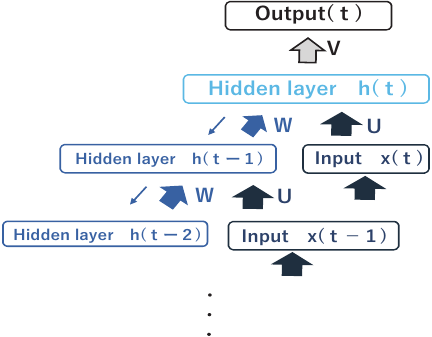
Fig. 1. Recurrent neural network structure.
The structure of the RNN used in this study is shown in Fig. 1. The RNN used in this study was a single-layer vanilla RNN with tanh activation. The network consists of an input layer, a hidden layer with recurrent connections, and an output layer. At each time step \(t\), the hidden state \(h(t)\) is computed from the current input \(x(t)\) and the previous hidden state \(h(t-1)\) through shared weight matrices \(U\) and \(W\). The output is obtained by applying a linear transformation \(V\) to the hidden state at the final time step. All weight matrices are shared across time steps, and during training, the output error is backpropagated through time using BPTT to update the network parameters.
The model input is defined as follows:
3.2. Introducing Sparsity
The sparse modeling of AI began with the proposal of structured learning by Ishikawa 7,8,9. Sparse modeling is an approach in which the absolute-value sums of link weights and biases (L1 norm) are introduced as regularization terms in the error function. This forces unnecessary link weights to approach zero, and thus only the necessary links are retained. This results in the natural extraction of the structure necessary for regression.
To produce a sparse BPTT model using L1 regularization, the following regularization term is added along with link \(U\) between the input and intermediate layers, link \(W\) between the intermediate layers, link \(V\) between the intermediate and output layers, and the respective biases \(b\) and \(c\) of the intermediate and output layers.
This eliminates links that do not contribute to regression and produces a simplified model. However, the sole application of L1 regularization generates excessively distributed representations, which reduce the interpretability of the model.
To address this issue, we introduced L2 regularization based on the hidden-layer output in addition to the L1 norm using the method proposed by Ishikawa 12. Specifically, we added the following term for the hidden-layer output \(h_j^{(t)}\):
By combining L1/L2 and selective regularization, as described above, we could better extract the important attributes of the environmental data while reducing the distributed representations compared to our previous method. The objective of this study was not to predict growth assessment but to facilitate analysis and visualization. Therefore, this method could estimate the environmental factors that contribute to growth assessment in strawberry cultivation with higher interpretability than previous methods.
3.3. Process of Sparse Modeling
We applied a series of five training procedures to the same RNN model to estimate the environmental factors contributing to the growth assessment of strawberries. These procedures do not represent independent modeling approaches but different regularization settings that are applied sequentially and comparatively within a unified framework. By applying these procedures step-by-step, we investigated how the introduction and combination of L1, L2, and selective regularization affected model sparsity, stability, and interpretability. The final procedure, which combines selective L1 and selective L2 regularization, constitutes the proposed method of this study.
(1) MSE
Baseline training in which only the MSE is used as the loss function.
(2) MSE \(+\) L1 regularization
L1 regularization is introduced to the link weights and biases to reduce unnecessary links.
(3) MSE \(+\) L1 regularization \(+\) L2 regularization
In addition to L1, L2 regularization is introduced into the hidden-layer output to achieve both sparsity and stability.
(4) MSE \(+\) L1 regularization \(+\) selective L2 regularization
L2 regularization is applied only to the parts of the hidden-layer outputs that have a small contribution.
(5) MSE \(+\) selective L1 regularization \(+\) selective L2 regularization
Selective regularization is applied to both the link weights and hidden-layer outputs to achieve the highest interpretability.
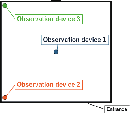
Fig. 2. Location of the observation devices.
4. Learning Conditions
4.1. Used Data
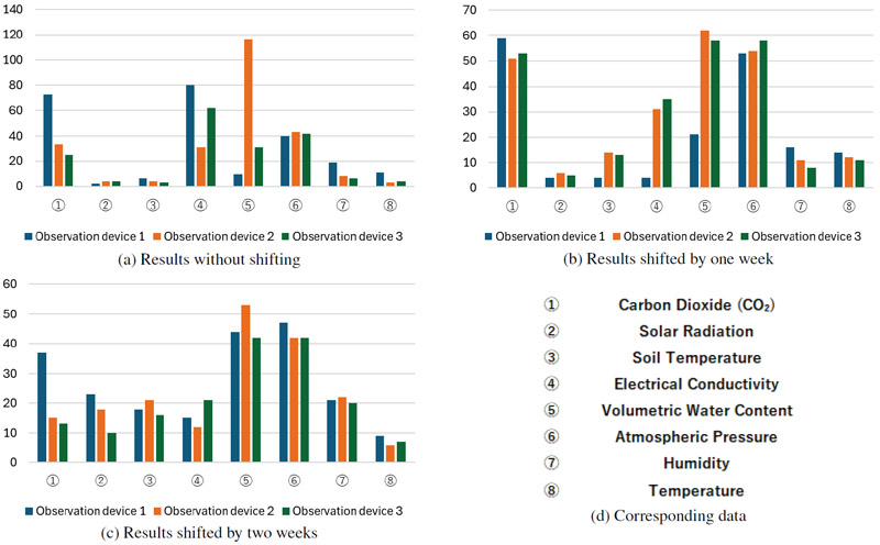
The data used in this study were divided into training and target data. The training data consisted of environmental data acquired by observation devices installed in an agricultural greenhouse and comprised eight types of data: carbon dioxide concentration, solar radiation, soil temperature, volumetric water content, electrical conductivity, humidity, temperature, and atmospheric pressure. Each observation device acquired data independently, and their locations are shown in Fig. 2.
The data were collected at 15-min intervals and adjusted to 72 samples per day for each attribute, with all values normalized to the range 0–1. For RNN training, these environmental data were not aggregated into a single daily input vector. Instead, they were arranged as multivariate time-series sequences using a sliding-window approach, in which consecutive environmental samples were stacked to form each input sequence, and the corresponding daily growth assessment was used as the target output. The target data were the growth assessment data provided by a farmer, which were used in this study as target variables for regression analysis rather than for prediction. They consisted of shipment volume, quality, growth status, and farmer intuition. Shipment volume was graded as either 0 (low) or 1 (high), whereas the other attributes were graded on a five-level scale and recorded once per day.
Three time periods were set for learning: the reference period between February 22 and March 17, 2025, a one-week-shifted period between March 1 and March 24, and a two-week-shifted period between March 8 and March 31. These were referred to as the no-shift, one-week-shift, and two-week-shift periods, respectively.
4.2. Learning Settings
In this experiment, the hyperparameters were unified to allow comparison of the results among the evaluation attributes.
Pre-training was conducted to induce sparsity and adjust the link weights and biases before the main training phase. The hyperparameters for pre-training and sparse modeling included a 16-dimensional input vector, 200 hidden-layer neurons, and a one-dimensional output, which were common to all attributes. Furthermore, the number of epochs for BPTT was set to 20,000, and the regularization intensities were set to 0.000005 for L1 and 0.000001 for L2. The other hyperparameters are presented in Table 1.
5. Learning Results
We evaluated three attributes: quality, growth status, and farmer intuition. Shipment volume was invariably given the highest score during the period in question and thus was excluded from factor estimation. In this paper, we focus on the results of quality, which showed a marked decline during the period under study. During the study period, the quality fell from five to two on a five-point scale, indicating a clear fluctuation in its assessment over time.
Figure 3 shows the experimental learning results for quality obtained via BPTT, as well as those obtained with L1/L2 and selective L1/L2 regularization. These results confirmed that regression was properly conducted. Based on the confirmation that regression would also be applicable to other attributes, we analyzed the link weights between the input and hidden layers to explore the causes of assessment variations.
Figure 4 shows the number of links with absolute weights exceeding the selective L1/L2 regularization thresholds for each input. The blue, orange, and green bars represent observation devices 1, 2, and 3, respectively. Because smaller link weights were mostly eliminated during the learning process, the input attributes associated with links exceeding the threshold were considered important for growth assessment.
Table 1. Learning conditions (hyperparameters).

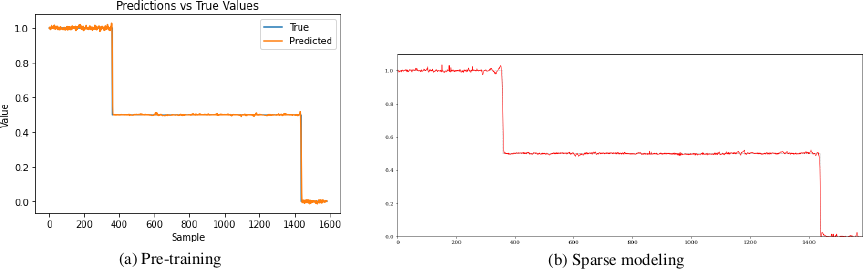
Fig. 3. Regression results for quality.
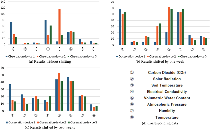
Fig. 4. Results for quality.
To determine the degree of influence for each device, thresholds were defined and the results were classified into four levels: “significant effect” (30 or more), “moderate effect” (20–29), “small effect” (10–19), and “no effect” (below 10). The results are summarized in Tables 2–4. Device 1 exhibited the greatest influence of atmospheric pressure and a notable effect of CO\(_2\) concentration. Device 2 was significantly affected by atmospheric pressure and volumetric water content, whereas the effects of CO\(_2\) concentration and electrical conductivity diminished in the two-week-shift period. Device 3 was also strongly influenced by the volumetric water content, whereas electrical conductivity had a strong effect, except in the two-week-shift period, where it became moderate. These results confirmed that atmospheric pressure had a strong influence on all observation devices. Additionally, device-specific tendencies were observed: device 1 was characterized by the influence of CO\(_2\) concentration, device 2 by changes in the effects of volumetric water content, CO\(_2\) concentration, and electrical conductivity, and device 3 by fluctuations in the effects of volumetric water content and electrical conductivity.
6. Discussion
In this study, we analyzed the effects of various inputs on growth assessment using learning results obtained across three periods shifted relative to each other. The input data cannot be directly compared with the evaluation data because they fluctuate widely. Therefore, the observation data were divided into groups of 24 items each, which were averaged to yield eight-hour averages, thus making them more comparable to the daily assessments. Here, we present two representative cases for discussion.
Table 2. Degree of influence on observation device 1 (quality).

Table 3. Degree of influence on observation device 2 (quality).

Table 4. Degree of influence on observation device 3 (quality).

6.1. Relationship Between Device 2 and Volumetric Water Content
First, we focus on the volumetric water content detected by observation device 2. Fig. 4 shows that this input had a significant effect across all three periods (with no shift, shifted by one week, and shifted by two weeks) and contributed in a stable manner to the quality assessment. Because the level of influence varied only slightly among the different learning periods, the volumetric water content can be considered a consistently important factor in quality assessment.
The observed data for device 2 and the evaluation data are compared in Fig. 5. For the no-shift period, the volumetric water content decreased in conjunction with the initial decline in quality, indicating its strong correspondence with quality. Furthermore, the volumetric water content gradually decreased during the remaining period, at which point the quality also gradually decreased. This suggests that in addition to its direct effect on quality, its gradual decrease may also have a continuous adverse effect on quality.
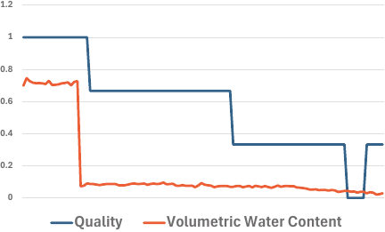
Fig. 5. Data on quality and volumetric water content.
From an agricultural standpoint, water is essential for the growth and maintenance of crop quality, and its prolonged shortage directly leads to reduced fruit development and the deterioration of external appearance. The findings of this study confirm the importance of maintaining stable volumetric water content in the context of crop management.
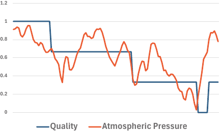
Fig. 6. Data on quality and atmospheric pressure.
Although electrical conductivity was also found to have a significant effect, this could be due to changes caused by the decreased volumetric water content. Because volumetric water content and electrical conductivity are closely related through their shared dependence on soil moisture conditions, we believe that the significant effect of electrical conductivity observed in this study was an indirect reflection of changes in the volumetric water content.
6.2. Relationship with Atmospheric Pressure
As shown in Fig. 4, the atmospheric pressure had a significant effect across all three periods. Because the atmospheric pressure data of the three observation devices were similar, we only focus on the results for device 1. Fig. 6 shows a comparison of the data from observation device 1 and quality assessment. The atmospheric pressure decreased whenever the quality decreased, and toward the end of the period shifted by two weeks, the quality showed a similar trend to the atmospheric pressure. These results suggest that atmospheric pressure had a consistent effect on quality assessment. However, little is known about the causal relationship between atmospheric pressure and crop quality, and the observational results of this study are insufficient to make definitive decisions on this matter. Because the observations acquired by the three devices, which were in close agreement, were treated as three attributes in the analysis, we plan to consolidate them using data from one representative device in the learning process. In the future, it may be necessary to incorporate farmers’ knowledge, conduct observations over an extended period, and collect further data to investigate how atmospheric pressure variations affect physiological responses and quality in strawberry cultivation.
7. Conclusions
The main contribution of this study is the construction of an intrinsically interpretable learning model for the identification and visualization of the environmental factors affecting strawberry cultivation, which may be superior to methods relying on post-hoc explanations for black-box predictors. By integrating structural learning into the training process through L1/L2 regularization, the proposed approach enables the direct interpretation of model parameters as meaningful cultivation-related factors. We analyzed the relationship between growth assessment values and environmental data obtained using multiple observation devices during strawberry cultivation. Using an RNN-based model with BPTT, structural sparsification was introduced during learning to extract the skeletal structure essential for regression. Consequently, the learned model structure itself served as an explanation of the decision-making process, allowing for factor identification without post-hoc analysis.
The analysis revealed that volumetric water content consistently had a significant influence on growth assessment, regardless of shifts in the learning period. This indicates that volumetric water content is a major and stable contributing factor to the evaluation of strawberry quality. In addition, atmospheric pressure had a significant influence across all observation devices and corresponded to fluctuations in growth assessment values. The magnitude of these effects differed depending on the device positions, suggesting that the spatial placement of the environmental sensors may affect the assessment results. Previous studies indicated that L1 regularization alone may retain moderately weighted parameters, which can reduce interpretability 10,11. In this study, this issue was mitigated by introducing structural learning that combines L1 and L2 regularizations, including selective regularization. This approach enabled stable sparse representations while suppressing excessively distributed features, thereby allowing the effective extraction of major environmental attributes with improved interpretability. Although the proposed method could identify meaningful cultivation factors, the results should not be interpreted as definitive agricultural conclusions.
Future work will involve the addition of observation devices to further examine the dependence on sensor placement. Furthermore, more detailed investigations into factors such as atmospheric pressure, whose agricultural significance is not yet fully understood, will be conducted. These efforts are expected to further validate the proposed framework and enhance its applicability to data-driven crop management and decision-support systems.
Acknowledgments
The authors would like to express their sincere gratitude to Mr. Nishimoto, a strawberry farmer who collected the data for this study and provided valuable insights, and to the staff at JA Fukuoka Keichiku for kindly referring us to him.
- [1] L. Droukas, Z. Doulgeri, N. L. Tsakiridis, D. Triantafyllou, I. Kleitsiotis, I. Mariolis, D. Giakoumis, D. Tzovaras, D. Kateris, and D. Bochtis, “A survey of robotic harvesting systems and enabling technologies,” J. of Intelligent & Robotic Systems, Vol.107, No.1, Article No.21, 2023. https://doi.org/10.1007/s10846-022-01793-z
- [2] Z. H. Wang, Y. Xun, Y. K. Wang, and Q. H. Yang, “Review of smart robots for fruit and vegetable picking in agriculture,” Int. J. of Agricultural and Biological Engineering, Vol.15, No.1, pp. 33-54, 2022. https://doi.org/10.25165/j.ijabe.20221501.7232
- [3] V. R. S. Rajendran, B. Debnath, S. Mghames, W. Mandil, S. Parsa, S. Parsons, and A. Ghalamzan-E, “Towards autonomous selective harvesting: A review of robot perception, robot design, motion planning and control,” J. of Field Robotics, Vol.41, No.7, pp. 2247-2279, 2023. https://doi.org/10.1002/rob.22230
- [4] M. K. A. Karkee and B. Adhikari, “Agricultural harvesting robot concept design and system components: A review,” Agronomy, Vol.5, No.2, Article No.48, 2024. https://doi.org/10.3390/agriengineering5020048
- [5] Y. Sugomori, “Deep learning explained in detail: Time series data processing with TensorFlow/Keras and PyTorch,” Mynavi Publishing, 2021 (in Japanese).
- [6] R. J. Williams and D. Zipser, “A learning algorithm for continually running fully recurrent neural networks,” Y. Chauvin and D. E. Rumelhart (Eds.), “Back-Propagation: Theory, Architectures and Applications,” Lawrence Erlbaum Associates, pp. 433-486, 1995.
- [7] M. Ishikawa, “Structured learning using forgetting in connectionist models,” IEICE Technical Report on Medical Electronics and Bio-Cybernetics (MEB88-144), pp. 143-148, 1988 (in Japanese).
- [8] M. Ishikawa, “Structural learning algorithm of connectionist model with forgetting,” J. of the Japanese Society for Artificial Intelligence, Vol.5, No.5, pp. 595-603, 1990 (in Japanese).
- [9] M. Ishikawa, “Structural learning with forgetting,” Neural Networks, Vol.9, No.3, pp. 509-521, 1996. https://doi.org/10.1016/0893-6080(96)83696-3
- [10] H. Hisatsune and K. Kamei, “Identification of growth factors in strawberries using sparse modeling AI,” Proc. of the 26th SOFT Kyushu Chapter Annual Conf., pp. 24-29, 2024 (in Japanese).
- [11] H. Hisatsune and K. Kamei, “Estimation of strawberry growth factors using sparse modeling AI,” Proc. of the 19th Int. Conf. on Innovative Computing, Information and Control (ICICIC 2025), p. 143, 2025.
- [12] M. Ishikawa, “Towards human-interpretable deep learning in stacked autoencoders,” IEICE Technical Report, pp. 99-104, 2019 (in Japanese).
- [13] A. Kamilaris and F. X. Prenafeta-Boldú, “Deep learning in agriculture: A survey,” Computers and Electronics in Agriculture, Vol.147, pp. 70-90, 2018. https://doi.org/10.1016/j.compag.2018.02.016
- [14] K. G. Liakos, P. Busato, D. Moshou, S. Pearson, and D. Bochtis, “Machine learning in agriculture: A review,” Sensors, Vol.18, No.8, Article No.2674, 2018. https://doi.org/10.3390/s18082674
- [15] A. Chlingaryan, S. Sukkarieh, and B. Whelan, “Machine learning approaches for crop yield prediction and nitrogen status estimation in precision agriculture: A review,” Computers and Electronics in Agriculture, Vol.151, pp. 61-69, 2018. https://doi.org/10.1016/j.compag.2018.05.012
- [16] T. Van Klompenburg, A. Kassahun, and C. Catal, “Crop yield prediction using machine learning: A systematic literature review,” Computers and Electronics in Agriculture, Vol.177, Article No.105709, 2020. https://doi.org/10.1016/j.compag.2020.105709
- [17] M. A. Jabed and M. A. A. Murad, “Crop yield prediction in agriculture: A comprehensive review,” Heliyon, Vol.10, No.24, Article No.e40836, 2024. https://doi.org/10.1016/j.heliyon.2024.e40836
- [18] S. P. Mohanty, D. P. Hughes, and M. Salathé, “Using deep learning for image-based plant disease detection,” Frontiers in Plant Science, Vol.7, Article No.1419, 2016. https://doi.org/10.3389/fpls.2016.01419
- [19] S. Sladojevic, M. Arsenovic, A. Anderla, D. Culibrk, and D. Stefanovic, “Deep neural networks based recognition of plant diseases,” Computational Intelligence and Neuroscience, Vol.2016, Article No.3289801, 2016. https://doi.org/10.1155/2016/3289801
- [20] T. Fujinaga, S. Yasukawa, and K. Ishii, “Tomato growth state map for the automation of monitoring and harvesting,” J. Robot. Mechatron., Vol.32, No.6, pp. 1279-1291, 2020. https://doi.org/10.20965/jrm.2020.p1279
- [21] K. Kase, N. Matsumoto, and T. Ogata, “Leveraging motor babbling for efficient robot learning,” J. Robot. Mechatron., Vol.33, No.5, pp. 1063-1074, 2021. https://doi.org/10.20965/jrm.2021.p1063
- [22] A. Bechar and C. Vigneault, “Agricultural robots for field operations: Concepts and components,” Biosystems Engineering, Vol.149, pp. 94-111, 2016. https://doi.org/10.1016/j.biosystemseng.2016.06.014
- [23] R. R. Shamshiri, D. Kalantari, K. C. Ting, J. R. Thorp, I. A. Hameed, and C. Weltzien, “Advances in greenhouse automation and controlled environment agriculture: A transition to plant factories and urban agriculture,” Int. J. of Agricultural and Biological Engineering, Vol.11, No.1, pp. 1-22, 2018. https://doi.org/10.25165/j.ijabe.20181101.3210
- [24] P. Filippi, B. M. Whelan, and T. F. A. Bishop, “Explainable machine learning to map the impact of weather and soil on wheat yield and revenue across the eastern Australian grain belt,” Agriculture, Vol.14, No.12, Article No.2318, 2024. https://doi.org/10.3390/agriculture14122318
- [25] K. Nagasubramanian, S. Jones, A. K. Singh, S. Sarkar, A. Singh, and B. Ganapathysubramanian, “Plant disease identification using explainable 3D deep learning on hyperspectral images,” Plant Methods, Vol.15, Article No.98, 2019. https://doi.org/10.1186/s13007-019-0479-8
- [26] S. M. Lundberg and S.-I. Lee, “A unified approach to interpreting model predictions,” Advances in Neural Information Processing Systems (NeurIPS), pp. 4765-4774, 2017.
- [27] M. T. Ribeiro, S. Singh, and C. Guestrin, “Why should I trust you?: Explaining the predictions of any classifier,” Proc. of the 22nd ACM SIGKDD Int. Conf. on Knowledge Discovery and Data Mining (KDD), pp. 1135-1144, 2016. https://doi.org/10.1145/2939672.2939778
- [28] C. Molnar, “Interpretable Machine Learning (2nd ed.),” Lulu Press, 2022.
- [29] F. Doshi-Velez and B. Kim, “Towards a rigorous science of interpretable machine learning,” arXiv:1702.08608, 2017. https://doi.org/10.48550/arXiv.1702.08608
- [a] Food and Agriculture Organization of the United Nations, “Employment indicators: Agriculture, forestry and fishing (2000–2023).” https://www.fao.org/statistics/highlights-archive/highlights-detail/employment-indicators-2000-2023-(july-2025-update)/ [Accessed January 20, 2026]
- [b] Ministry of Agriculture, Forestry and Fisheries, “Statistics on agricultural labor force.” https://www.maff.go.jp/j/tokei/sihyo/data/08.html [Accessed September 25, 2025]
- [c] Ministry of Agriculture, Forestry and Fisheries, “Preparation and start-up support funds for new farmers.” https://www.maff.go.jp/j/new_farmer/n_syunou/roudou.html [Accessed September 25, 2025]
- [d] Grand View Research, “Harvesting robots market size, Share & Trends analysis report.” https://www.grandviewresearch.com/industry-analysis/harvesting-robots-market-report [Accessed January 28, 2026]
This article is published under a Creative Commons Attribution-NoDerivatives 4.0 Internationa License.