Paper:
Development of a Map-Based Energy Consumption Model for Orchard Electric Vehicles Using Field Data
Tomoaki Hizatate*
 and Noboru Noguchi**
*Graduate School of Agriculture, Hokkaido University
Kita 9, Nishi 9, Kita-ku, Sapporo, Hokkaido 060-8589, Japan
**Research Faculty of Agriculture, Hokkaido University
Kita 9, Nishi 9, Kita-ku, Sapporo, Hokkaido 060-8589, Japan

This study presents a novel map-based energy consumption prediction model for agricultural electric vehicles operating in real orchard environments. Traditional static models often overlook resistance factors caused by varying terrain and soil conditions. To address this, we introduce an unknown resistance component Fu, mapped spatially to reflect local environmental influences such as slope and soil hardness. Field experiments were conducted in a vineyard in Hokkaido, Japan, using GNSS and battery data collected at 10 Hz during uphill and downhill runs. The proposed model achieved a maximum mean absolute percentage error of 2.3%, significantly outperforming conventional models. A notable negative correlation between Fu and soil hardness was observed, confirming that softer soils increase vehicle resistance. Simulations of continuous operations across adjacent routes further demonstrated reduced cumulative prediction errors, supporting applications in route planning and battery management. Fu(x,y) is currently treated as static, and future work will expand it to a spatiotemporal parameter Fu(x,y,t) to incorporate dynamic environmental changes. Online learning and validation across diverse terrains are also planned. This approach enhances model adaptability, offering a reliable tool for energy-efficient and sustainable operation of electric vehicles in agriculture.
Mapping unknown resistance onto grid from driving data
1. Introduction
Along with recent advances in agricultural vehicle automation and precision farming, these technologies have garnered increasing attention as a means of achieving more efficient agricultural production 1. Their application may be particularly suited to orchard operations, which involve not only routine tasks such as weeding and pesticide applications but also a variety of labor-intensive manual tasks. In Japan, fruit production accounts for nearly 10% of the total agricultural output value, with grapes, citrus, and apples representing more than half of the sector a. Despite this economic importance, a large proportion of orchard work hours is still devoted to manual tasks such as pruning, thinning, and harvesting, which remain difficult to mechanize. These tasks are heavily dependent on the availability of seasonal workers, making production planning highly susceptible to fluctuations in weather conditions and labor availability. As a result, this labor dependence poses a significant challenge to the realization of sustainable agricultural management. Furthermore, since fruit trees require long-term management, orchard growers have been less inclined to expedite the adoption of advanced technologies, leading to a technology deficit and urgent need for improved operational efficiency.
In addition, growing global concern over environmental issues has led to increasing demands to reduce the environmental impact of agricultural practices. Fuel consumption and exhaust emissions from agricultural vehicles are recognized as significant contributors to this impact, prompting a global shift toward electrification. Major agricultural machinery manufacturers such as Kubota and John Deere have released commercial electric tractors b,c, and in recent years, companies specializing exclusively in electric agricultural vehicles have also emerged d.
Electric agricultural vehicles not only produce zero greenhouse gas emissions and harmful exhaust during operation—thereby significantly reducing environmental impact—but also offer structural simplicity by eliminating the need for fuel, resulting in lower fuel and maintenance costs. Furthermore, their ability to deliver maximum torque even at low speeds enables stable power output, making them well-suited for integration with the Internet of Things and autonomous driving technologies that support precision agriculture.
Compared to conventional vehicles, electric agricultural vehicles still face limitations in terms of driving range and power supply to attached implements. However, their application is particularly promising in environments such as orchards, where heavy traction tasks like plowing are uncommon, and as outdoor utility vehicles [2, d].
To fully leverage the performance of electric agricultural vehicles, the optimization of travel paths and work scheduling is becoming increasingly important. Orchards are often located in mid-mountainous areas due to favorable drainage and sunlight conditions. As a result, compared to the flat fields typical of most crop farms, these orchards tend to have steeper slopes, and work efficiency is highly dependent on the quality of the operational planning.
Challenges related to the steeper terrains generally fall into two categories: coverage path planning (CPP) and the vehicle routing problem (VRP). CPP focuses on planning explicit routes that allow mobile units—such as combines, tractors, or drones—to cover the entire field without omission. CPP-based methods have been applied to the coverage of irregularly shaped fields 3, obstacle avoidance within fields 4, and minimization of non-working times such as turning at headlands 5, among others 6.
In contrast, VRP is defined as the problem of optimizing a value, such as total travel distance or time, by determining the optimal visiting order and routes among multiple points (e.g., field locations or workstations). Numerous VRP studies have addressed the optimization of task scheduling for heterogeneous fleets 7,8 coordinated operations among multiple vehicles 9, master–follower planning for harvest and transport robots 10, and task time optimization under performance constraints of vehicles or implements 2,11. Studies focusing on electric robotic vehicles have formulated VRPs that account for energy consumption 11,12, reflecting the practical limitations imposed by their relatively short operating range.
However, most existing studies have primarily relied on simulations based on mathematical models, and few have discussed how the accuracy of these models impacts task planning under real-world conditions. Particularly in agricultural fields, where factors such as unpaved surfaces and sloped terrain introduce nonlinearities and high uncertainty, conventional models have struggled to adequately represent the environmental complexity.
To address this problem, we here apply the VRP framework to battery-powered electric agricultural vehicles for more accurate energy consumption estimation. We propose a method that addresses localized error factors—unaccounted for in conventional static energy consumption models—by geographically mapping them as position-dependent parameters. Rather than fundamentally altering the structure of the conventional model, our approach incrementally accumulates and corrects estimation errors based on actual driving data, thereby indirectly reflecting the unique terrain and surface conditions of the field. We validate the method against conventional static models using real driving data collected from an orchard, and show that the corrective mapping improved prediction accuracy under complex environmental conditions. Finally, we outline future extensions to capture temporal variations such as soil moisture and terrain changes.
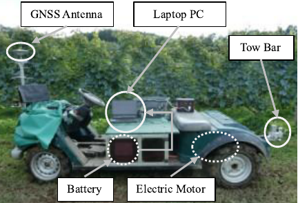
Fig. 1. Sensor and system configuration.
Table 1. Characteristics of the system and sensors.

2. Materials and Methods
2.1. System Configuration
In this study, we used an electric vehicle based on a golf cart, as shown in Fig. 1, to collect actual energy consumption and positioning data in agricultural fields. The vehicle is equipped with an electric motor recycled from the powertrain of a hybrid car; Table 1 summarizes its main specifications. A tow bar is installed at the rear of the vehicle, allowing it to pull agricultural implements such as sprayer, mower, and trailer.
To measure the vehicle’s positioning state, a real-time kinematic global navigation satellite system (RTK-GNSS) was mounted on the vehicle, enabling position information with centimeter-level accuracy. In this experiment, the centimeter-level augmentation service (CLAS) was applied, which provided stable centimeter-level positioning throughout all runs. Although global navigation satellite system (GNSS) degradation can occur in orchard environments due to canopy or terrain effects, no significant signal loss or positioning instability was observed at the experimental field. The vehicle was also equipped with a battery management system (BMS) that acquired output voltage and current in real time; this allowed precise calculation of instantaneous power consumption, which could be correlated with the position data.
For data collection, a laptop computer was installed on the vehicle to synchronize and record GNSS position data and BMS voltage and current outputs. These data were then utilized for constructing and evaluating the energy consumption model described later.
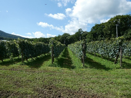
Trellis rows are spaced at 2.5-m intervals, and the vehicle operates autonomously between the rows.
Fig. 2. A schematic view of the vineyard for wine grapes.
2.2. Problem Description
We sought to develop a system that more accurately predicts energy consumption in electric agricultural vehicles and can ultimately be applied to solve the VRP for robotic agricultural vehicles. Generally, when solving the VRP, a task-space map is provided as prior knowledge and used to optimize the operation time and energy consumption. Accordingly, this study assumes the availability of a pre-acquired digital terrain map (DTM) of the field, which reflects physical features such as terrain, slope, and undulation.
The target site for this study was a vineyard (Fig. 2). Vines were planted at 2.5-m intervals, and the vehicle traveled along routes drawn between the rows. As shown in Fig. 3, the field was sloped, with a downhill gradient from the starting point to the end point.
The vehicle traveled along predetermined routes drawn on the 3D map, following a specified traversal sequence. For example, if the order was given as 1, 6, 2, 7, the vehicle first traveled along route No.1 from the start point to the end point, then performed a turning maneuver in the headland area, and subsequently traveled along route No.6 from the end point back to the start point. By repeating this process, the assigned tasks were executed. The sequence of route traversal was optimized by solving the VRP to minimize operation time and energy consumption.
In this study, we propose an approach in which the parameters of the energy consumption model are updated using actual driving data each time the vehicle completes a single route. This method allows for the sequential incorporation of environmental effects that conventional models fail to capture, thereby providing a flexible energy consumption model suitable for practical operation.
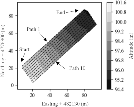
Several vehicle routes (dashed lines), each \(\sim 100\) m in length and oriented from southwest to northeast. There is an elevation difference of \(\sim 7\) m between the start and end points of each route.
Fig. 3. Digital terrain map (DTM) of the vineyard.
2.3. Definition of the Energy Consumption Model
In general, the external forces acting on a vehicle during travel include rolling resistance, aerodynamic drag, gradient resistance, and acceleration resistance 13,14. However, since agricultural vehicles typically operate at low and steady speeds, the effects of aerodynamic drag and acceleration resistance are considered negligible and thus omitted. Therefore, the primary external forces considered are rolling resistance \(F_{r}\) and gradient resistance \(F_{s}\).
In actual agricultural environments, however, it is difficult to accurately describe energy consumption using only these theoretical forces. For example, the test vehicle was rear-wheel drive, and during operation on slopes, the vertical load on the rear wheels varied, altering the tire-ground interaction. Additionally, the terrain featured local irregularities and temporal changes in surface conditions, introducing strong nonlinearities.
To account for such real-world factors, this study introduces an unknown resistance component \(F_{u}\) in addition to the conventional rolling and gradient resistances. \(F_{u}\) functions as a buffer parameter representing external forces that cannot be explained by rolling or gradient resistance alone—specifically, resistance components arising from terrain characteristics. Since \(F_{u}\) is closely related to road surface conditions and geographical features, it is assumed to have spatiotemporal dependency. For simplicity, however, this study considers only spatial dependency and defines \(F_{u}\) as a parameter that varies according to the vehicle’s position.
Using these resistance components, the instantaneous battery output power \(P(x,y)\) at position \((x,y)\) can be formulated as follows:
Here, \(\eta\) represents the loss coefficient due to internal vehicle resistances, encompassing all forms of energy loss such as electrical resistance loss, mechanical friction loss, and control system loss. Using Eq. \(\eqref{eq:eq1}\), the amount of energy consumed \(E\) over the time interval from \(t_{0}\) to \(t_{1}\) is expressed as follows:
Moreover, to explicitly account for the effects of load variation caused by slope inclination, the model incorporates the following two complementary methodologies:
2.4. Methodologies for Updating the Parameter
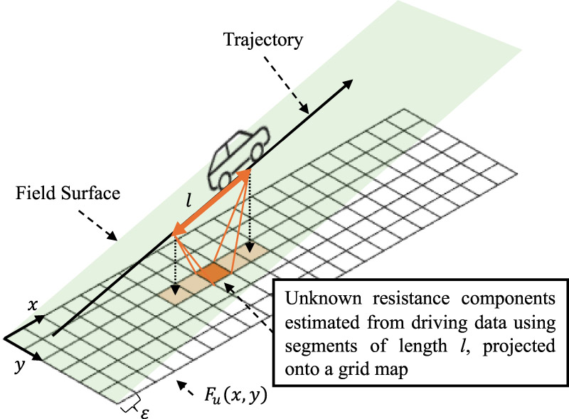
In this study, to manage the unknown resistance component \(F_{u}\) spatially, the field was divided into multiple grid cells, each with a side length of \(\varepsilon\), forming a grid map \(F_{u}(x,y)\). Each grid cell stored the value of the unknown resistance component corresponding to that location. After the vehicle completed one route traversal, the values of the grid cells along the travel trajectory were updated. Fig. 4 illustrates this method.
Assuming that \(F_{u}\) is constant as \(\tilde{F}_{u}\) over any segment of length \(l\) along the travel trajectory, the energy consumed within that segment (designated \(E_{m}\)), as obtained from the BMS, can be expressed as follows:
Since \(\tilde{F}_{u}\) represents the residual obtained by subtracting the rolling resistance and gradient resistance from the observed energy consumption, it can be calculated by inverse estimation.
By updating the model parameters based on location in this manner, the model reflects the actual operating environment, thereby improving the accuracy of energy consumption prediction.
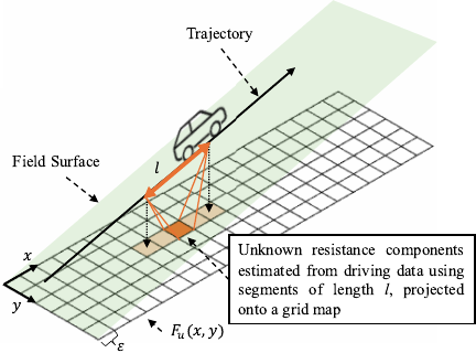
Fig. 4. Mapping of unknown resistance \(F_{u}(x,y)\) onto a grid map based on driving data.
2.5. Methodologies for Estimating Energy Consumption
The method for estimating energy consumption on unknown routes based on prior knowledge of the DTM and vehicle parameters is as follows. The route, which is the target for energy consumption estimation obtained from the DTM, is represented as
The total travel distance, horizontal travel distance, and vertical travel distance between each pair of points along the route are expressed as follows:
By transforming Eq. \(\eqref{eq:eq3}\) using Eq. \(\eqref{eq:eq8}\), the estimated energy consumption \(\hat{E}\) along the route expressed in Eq. \(\eqref{eq:eq5}\) can be represented using the unknown parameter map \(F_{u}(x,y)\) as follows:
As shown in Eq. \(\eqref{eq:eq9}\), the value of \(F_{u}(x,y)\) was assigned based on the value stored in the grid cell nearest to the target position for estimation.
Table 2. Parameters used in the model.

2.6. Experimental Method
The proposed method was validated at the Shiribeshi Vineyard owned by Hokkaido Wine in Niki, Hokkaido. Ten distinct straight routes, each approximately 100 m in length, were set up for the test. The vehicle was manually operated at a constant speed of about 0.8 m/s. Since the routes were sloped along the direction of travel, two sets of runs—uphill and downhill—were conducted, resulting in a total of 20 runs. The data collected during the runs consisted of position information obtained from GNSS and energy consumption data from the BMS. Both GNSS and BMS data were recorded at a frequency of 10 Hz. To verify that \(F_{u}\) depends on geographical factors, soil hardness was measured approximately every 5 m along the routes using a soil hardness tester (Yamanaka Standard type, Fujiwara Scientific Co., Ltd., Japan). At each measurement point, surface soil hardness was measured by taking five readings at the center of the route, where no vegetation was present and no wheel load had been applied, and the average value was used for analysis.
The parameters used in the model are shown in Table 2. As indicated in Table 2, a 1-m grid map was employed in this study. The estimation of \(F_{u}\) was performed using driving data collected over 5 m segments, and the estimated value was assigned to the grid cell corresponding to the midpoint of each segment. These spatial resolutions were appropriate for smoothing instantaneous noise while still capturing localized variations in terrain conditions.
The value of \(C_{r}\) was adopted from the estimation reported in 14 as the same vehicle and tire configuration used in the previous study was employed in the present experiment. The value of \(\eta\) was determined through regression under the assumption that \(C_{r}\) was 0.043 (based on 14) and that \(F_{u}\) was zero, i.e., no unknown resistance components, on a flat asphalt pavement. The regression coefficient was calculated as 0.99.
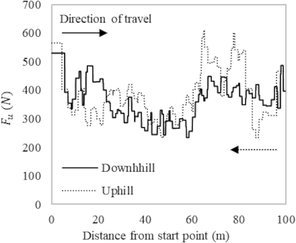
Fig. 5. Mapping of the unknown resistance \(F_{u}\) along the route No.3.
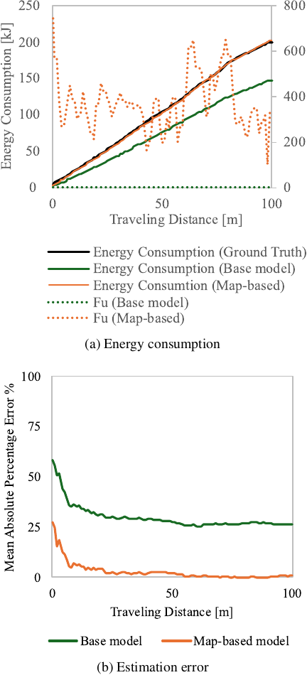
Fig. 6. Comparison of energy consumption estimation and error analysis.
3. Results and Discussion
3.1. Variation of \(F_{u}\) Along the Route
Figure 5 shows the spatial mapping of the unknown resistance component \(F_{u}\) along the driving route. The vertical axis represents the value of \(F_{u}\), while the horizontal axis indicates the distance along the route. The dotted line corresponds to the parameters measured during uphill travel, and the solid line represents those during downhill travel.
The results demonstrate that the values of \(F_{u}\) vary significantly depending on the location along the route, and a distinct difference is observed between uphill and downhill conditions. This can be attributed to the change in load distribution on the rear wheels of the rear-wheel-drive vehicle caused by the slope, which affects the motor load and resistance components.
These findings highlight the necessity of clearly separating the uphill and downhill cases within the model, supporting the robustness of the proposed modeling framework.
3.2. Comparison of Energy Consumption Estimation Methods
Next, the accuracy of the proposed method was evaluated using adjacent routes. Because the surface conditions in the orchard exhibit strong continuity along the row direction, factors such as soil hardness, surface roughness, and slope geometry do not change substantially within approximately 2.5 m. Therefore, adjacent routes can be regarded as having similar terrain characteristics and were used for comparative estimation.
Specifically, the unknown resistance component \(F_{u}(x,y)\) estimated from data on route No.3 was used to predict the energy consumption for route No.4. Fig. 6(a) shows the distance along the driving route on the horizontal axis, with the left vertical axis representing the energy consumption during route traversal and the right vertical axis showing the unknown resistance component \(F_{u}\). The figure compares the measured data (ground truth), the estimation results from the proposed method (map-based), and a static model that assumes zero unknown resistance component (baseline). Fig. 6(b) presents the mean absolute percentage error (MAPE) of energy consumption for each method, comparing the relative magnitude of estimation errors.
The results indicate that the proposed method closely matches the ground truth, demonstrating high estimation accuracy. Although energy consumption increases almost linearly with travel distance, nonlinear fluctuations were observed at certain points. These fluctuations reflect the strongly nonlinear environmental factors present in the actual field, such as surface unevenness and slope changes in the farmland.
Since the static model does not account for the unknown resistance component, it fails to capture such nonlinear fluctuations, resulting in an underestimation of energy consumption. In contrast, the proposed method flexibly accommodates these nonlinear variations by mapping the unknown resistance component to reflect real environmental changes.
These findings suggest that a model capable of dynamically reflecting unknown environmental factors is indispensable when planning tasks and routes under real-world field conditions. Furthermore, improving model accuracy directly contributes to appropriate battery capacity assessment and maximization of operational efficiency, highlighting the need for further acquisition of detailed environmental data and validation under diverse conditions.
Table 3 shows the maximum, minimum, mean, and standard deviation of the MAPE when estimating energy consumption for adjacent routes. These results confirm that the proposed method can estimate energy consumption with high accuracy for both the uphill and downhill cases. This is likely because the soil–tire interactions were similar between these geographically adjacent routes. Notably, the model exhibited exceptionally high accuracy under the uphill conditions, with greater error for the downhill case.
Table 3. Maximum, minimum, mean, and standard deviation of the mean absolute percentage error (MAPE) in energy consumption estimation between adjacent routes.

However, some routes—specifically routes 5 and 9—showed poor performance both as estimation targets and as estimation sources. Table 4 presents the average power consumption for each route, and routes 5 and 9 exhibited noticeably lower values compared with the others. This discrepancy is likely attributable to inconsistencies in the quality of manual driving during data collection. If the vehicle were operated under autonomous control rather than manual driving, the consistency of speed regulation would likely improve, potentially enhancing estimation accuracy. This observation also suggests that the performance of the speed controller plays an important role in the reliability of the estimation.
On the other hand, the proposed method estimates unknown route conditions by referring to the nearest grid cell values of \(F_{u}(x,y)\). However, for highly localized terrain irregularities or road surface conditions that are not consistent between routes, this approach faces limitations. Therefore, introducing alternative estimation methods will be necessary in future work.
Furthermore, in downhill scenarios, the vehicle has the potential to regenerate energy, which the proposed model does not yet accurately capture. Since regenerative behavior during downhill driving exhibits dynamics distinct from existing models, dedicated modeling approaches will need to be considered in future research.
Figure 7 shows the results of applying the uphill parameterization of the energy consumption model, \(E_{\mathit{uphill}}\), to estimate energy consumption during downhill driving. Compared with the actual consumption data, the estimated values deviated significantly, clearly failing to capture the decreasing trend in energy consumption observed during downhill operation.
This discrepancy is considered to arise from the fundamentally different external forces acting on the vehicle during uphill and downhill driving. For a rear-wheel-drive vehicle, the load distribution on the rear wheels changes due to slope inclination, which substantially affects the motor load, the rolling resistance, and the unknown resistance component \(F_{u}\). While uphill driving increases rear-wheel load and requires higher tractive effort, downhill driving shifts the load toward the front wheels, while reducing it on the rear wheels. Applying the same parameterization to both conditions thus results in an overestimation during downhill driving.
These findings demonstrate the necessity and validity of clearly separating uphill and downhill cases within the model. They also suggest that recognizing the distinct dynamic characteristics according to slope direction is crucial for understanding the energy consumption behavior of electric agricultural vehicles.
Future work should address more detailed modeling, including transitions between the uphill and downhill cases and accommodating intermediate slope conditions.
Table 4. Average power consumption for each route.

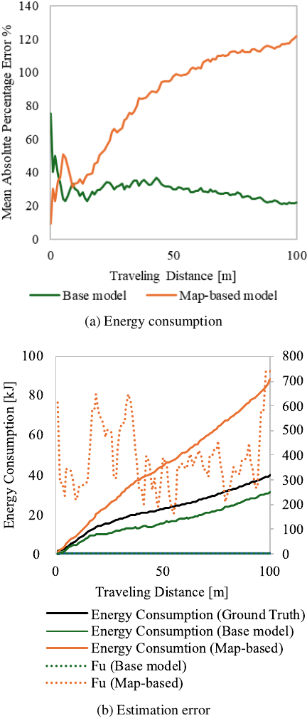
Fig. 7. Energy consumption estimation using the uphill parameterization for downhill running.
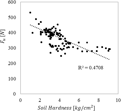
Fig. 8. Correlation between soil hardness and unknown resistance \(F_{u}\).
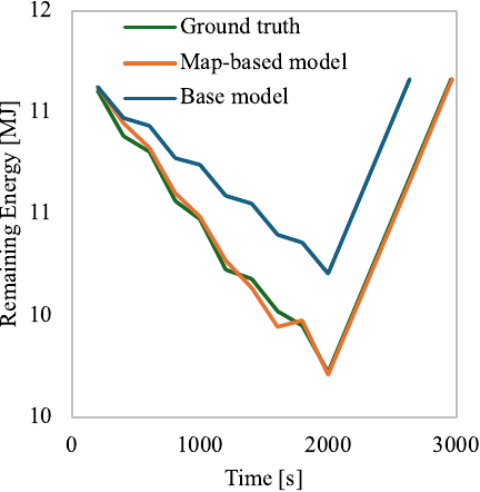
Fig. 9. Simulation of energy consumption dynamics over multiple routes.
3.3. Correlation Between Soil Hardness and Unknown Resistance \(F_{u}\)
Figure 8 illustrates the relationship between soil hardness along the route and the unknown resistance component \(F_{u}\). The analysis revealed a negative correlation between the two variables, indicating that higher soil hardness (i.e., harder soil) tends to correspond to lower values of \(F_{u}\). The coefficient of determination \(R^{2} = 0.47\) suggests a moderate explanatory power, meaning that soil hardness accounts for approximately 47% of the variation in the unknown resistance component.
This negative correlation is thought to reflect the fact that softer soils cause greater ground deformation and tire sinkage, which in turn increases the unknown resistance component \(F_{u}\) acting on the vehicle. Conversely, harder soils result in less vehicle sinkage and comparatively lower resistance, thereby suppressing increases in energy consumption.
However, as the \(R^{2}\) value remains at 0.47, it is evident that environmental factors other than soil hardness also significantly influence the variation in \(F_{u}\). For example, unevenness of the terrain, soil moisture, slope angle, tire tread patterns, and the condition of attached implements are among the diverse factors likely interacting in complex ways.
Therefore, in future investigation we plan to incorporate environmental data beyond soil hardness and employ multivariate analysis or machine learning techniques to further analyze the unknown resistance component.
3.4. Simulation of Real-World Operation Scenarios
Figure 9 shows the simulation results that emulate a scenario where the vehicle consecutively traverses 10 routes and subsequently undergoes a full recharge in preparation for the next task. The horizontal axis represents time, while the vertical axis indicates the cumulative energy consumption. The figure compares the ground truth (measured data), the estimation results from the proposed method, and a conventional offline estimation method (baseline) that does not consider the unknown resistance component \(F_{u}\).
The proposed method achieves high estimation accuracy by integrating actual driving data with the energy consumption model, closely reproducing the temporal changes in energy consumption observed in the measured data.
In contrast, the conventional model, which completely neglects the unknown resistance component \(F_{u}\), tends to underestimate the total energy consumption. This underestimation becomes more pronounced toward the latter part of the driving sequence, where errors accumulate and the discrepancy between estimated and actual consumption grows significantly.
Moreover, when comparing the actual task completion time with the estimated completion time, the proposed method yielded an error of only 9 seconds, whereas the conventional method exhibited a much larger error of 323 seconds. This demonstrates the clear superiority of the proposed method even under the relatively short test conditions, i.e., 10 routes of approximately 100 m each (totaling about 1 km).
These results suggest that the proposed model has the potential to deliver even greater performance in real-world environments requiring larger fields and longer operation times. Particularly for the operation of electric agricultural vehicles, where accurate estimation of battery replacement or intermediate charging timing is essential, the importance of a highly accurate predictive model adapted to actual driving conditions is strongly underscored. Moreover, high-accuracy estimation of route-level energy consumption enables practical applications such as predicting remaining working time, optimizing intermediate charging locations, and improving battery management strategies for electric agricultural vehicles.
3.5. Limitations and Future Works
In this study, we introduced an unknown resistance component \(F_{u}\), which captures prediction errors that conventional static energy models fail to address, and treated it as a spatial parameter dependent on position. This approach improved the accuracy of energy consumption prediction on untraveled routes. It was particularly effective in compensating for errors caused by spatially continuous environmental factors such as slope and soil conditions, thereby enhancing prediction accuracy for adjacent travel routes within the same field and time.
However, temporal variations in environmental conditions—such as soil moisture, surface irregularities, and field disturbance after operations—cannot be ignored. For example, data obtained at different times, such as after rainfall or during dry periods, pose limitations to treating \(F_{u}(x,y)\) as a fixed value. Such dynamic environmental changes can cause abrupt fluctuations in energy consumption, and scenarios where static spatial mapping alone is insufficient for accurate estimation are conceivable.
Future research should focus on extending the model to incorporate such temporal variations. One promising direction is to formulate \(F_{u}\) as a function of not only space but also time, i.e., \(F_{u}(x,y,t)\), enabling the model to flexibly respond to changing environmental conditions. Such temporal extensions would also enable application to robots whose mass changes over time, such as harvesting transport robots or pesticide-spraying robots. Additionally, incorporating online learning and sequential parameter updating methods could facilitate real-time adaptation utilizing prior driving data.
Furthermore, as the current validation is limited to specific fields and conditions, applying this approach to diverse fields with varying terrain and climatic conditions to evaluate model generalizability is a crucial future task. Especially when considering practical deployment for VRP, highly accurate estimation of energy consumption for each travel route will significantly influence multiple factors such as route selection, task sequencing, and charging strategies, thus necessitating more reliable model development.
The model applied in this study does not account for lateral motion or maneuvers involving acceleration and deceleration, such as turning operations. For this study, travel segments during turning maneuvers were not considered in the estimation, as the focus was on energy consumption during straight-line motion. This simplification was adopted because such motions occur over short distances and represent only a small proportion of total energy consumption. Although these effects may be partially buffered by \(F_{u}\), incorporating models that explicitly consider steering resistance, acceleration, and deceleration would enable more detailed estimation and expand applicability across the entire field.
Overall, our present results show that the proposed error compensation method based on spatially dependent parameters represents a meaningful step toward improving energy consumption models under real-world conditions. Going forward, incorporating temporal factors and validating the model under broader conditions should substantially improve the practical optimization of operation planning for electric agricultural vehicles.
4. Conclusion
In this study, we proposed a method to improve the accuracy of energy consumption prediction for electric agricultural vehicles operating in real field environments by introducing unknown factors—unaddressed by conventional static models—as spatially dependent parameters. The proposed model incorporates geographic and physical environmental factors, such as terrain and road surface conditions, difficult to express with previous models, as position-dependent unknown resistance components \(F_{u}\). This enables correction of rolling resistance and gradient resistance, achieving energy consumption estimates that more accurately reflect real-world conditions.
Evaluation experiments demonstrated that the proposed method achieved low error relative to the ground truth, with a maximum relative error of 2.3%. Moreover, the negative correlation found between \(F_{u}\) and soil hardness confirmed that the method captured the nonlinear influences of terrain and soil conditions. This suggests that static energy models alone may not provide sufficient accuracy in highly uncertain agricultural field environments.
Furthermore, simulations mimicking actual operations showed a significant reduction in cumulative energy consumption errors when using the proposed method. The prediction error of task completion time improved markedly—from 323 seconds with the conventional method to only 9 seconds with the proposed method—demonstrating the practical value of the approach for route optimization and work scheduling.
However, the unknown resistance component \(F_{u}(x,y)\) in this study is defined as a static parameter depending only on spatial position, limiting responsiveness to temporally varying environmental factors such as soil moisture and road surface irregularities. Extension of the model to spatiotemporal formulations \(F_{u}(x,y,t)\) and incorporation of online learning for sequential parameter updates remain subjects for future work.
Since the current validation was conducted in a limited field environment, applying the proposed model to larger datasets covering diverse terrains and climatic conditions will be necessary to evaluate its generalizability. Ultimately, we aim to apply this model to VRP for electric agricultural vehicles, enabling energy-constrained optimal work planning. We hope that this framework will provide a foundational approach for developing adaptive and practical prediction models suited to real-world environments.
Acknowledgments
This research is supported by the Research Promotion Program for Enhancing Innovative Creation funded by the Bio-oriented Technology Research Advancement Institution (BRAIN). The project is named “Development of a smart grapevine cultivation system using electric robots (03020C1).”
- [1] N. Noguchi, “Agricultural vehicle robot,” J. Robot. Mechatron., Vol.30, No.2, pp. 165-172, 2018. https://doi.org/10.20965/jrm.2018.p0165
- [2] T. Hizatate and N. Noguchi, “Work schedule optimization for electric agricultural robots in orchards,” Comput. Electron. Agric., Vol.210, Article No.107889, 2023. https://doi.org/10.1016/J.COMPAG.2023.107889
- [3] T. Oksanen and A. Visala, “Coverage path planning algorithms for agricultural field machines,” J. Field Robot., Vol.26, No.8, pp. 651-668, 2009. https://doi.org/10.1002/ROB.20300
- [4] K. Zhou, A. L. Jensen, C. G. Sørensen, P. Busato, and D. D. Bothtis, “Agricultural operations planning in fields with multiple obstacle areas,” Comput. Electron. Agric., Vol.109, pp. 12-22, 2014. https://doi.org/10.1016/J.COMPAG.2014.08.013
- [5] D. D. Bochtis and S. G. Vougioukas, “Minimising the non-working distance travelled by machines operating in a headland field pattern,” Biosyst. Eng., Vol.101, No.1, pp. 1-12, 2008. https://doi.org/10.1016/J.BIOSYSTEMSENG.2008.06.008
- [6] A. Utamima and A. Djunaidy, “Agricultural routing planning: A narrative review of literature,” Procedia Comput. Sci., Vol.197, pp. 693-700, 2022. https://doi.org/10.1016/J.PROCS.2021.12.190
- [7] J. Conesa-Muñoz, J. M. Bengochea-Guevara, D. Andujar, and A. Ribeiro, “Efficient distribution of a fleet of heterogeneous vehicles in agriculture: A practical approach to multi-path planning,” 2015 IEEE Int. Conf. on Autonomous Robot Systems and Competitions, pp. 56-61, 2015. https://doi.org/10.1109/ICARSC.2015.39
- [8] S. Li et al., “Intelligent scheduling method for multi-machine cooperative operation based on NSGA-III and improved ant colony algorithm,” Comput. Electron. Agric., Vol.204, Article No.107532, 2023. https://doi.org/10.1016/J.COMPAG.2022.107532
- [9] N. Wang et al., “Collaborative path planning and task allocation for multiple agricultural machines,” Comput. Electron. Agric., Vol.213, Article No.108218, 2023. https://doi.org/10.1016/j.compag.2023.108218
- [10] N. Noguchi, “Work schedule creation for agricultural mobile robots using genetic algorithms,” IFAC Proc. Volumes, Vol.32, No.2, pp. 5587-5591, 1999. https://doi.org/10.1016/S1474-6670(17)56952-9
- [11] Y. Xu et al., “Path planning and scheduling of multiple unmanned ground vehicles for orchard plant protection operations,” Comput. Electron. Agric., Vol.237, Part B, Article No.110615, 2025. https://doi.org/10.1016/J.COMPAG.2025.110615
- [12] M. Vahdanjoo, R. Gislum, and C. A. G. Sørensen, “Three-dimensional area coverage planning model for robotic application,” Comput. Electron. Agric., Vol.219, Article No.108789, 2024. https://doi.org/10.1016/j.compag.2024.108789
- [13] J. Romero Schmidt and F. Auat Cheein, “Assessment of power consumption of electric machinery in agricultural tasks for enhancing the route planning problem,” Comput. Electron. Agric., Vol.163, Article No.104868, 2019. https://doi.org/10.1016/j.compag.2019.104868
- [14] Y. Yamasaki, K. Ishii, and N. Noguchi, “Speed control of an autonomous electric vehicle for orchard spraying,” Comput. Electron. Agric., Vol.236, Article No.110419, 2025. https://doi.org/10.1016/J.COMPAG.2025.110419
- [a] Ministry of Agriculture, Forestry and Fisheries (MAFF), “Kaju wo meguru josei” [Fruit production trends in Japan], 2025 (in Japanese). https://www.maff.go.jp/j/seisan/ryutu/fruits/index.html [Accessed January 14, 2026]
- [b] Kubota, “Compact tractors Kubota LXe series.” https://kuk.kubota-eu.com/groundcare/series/lxe-series/ [Accessed September 12, 2025]
- [c] John Deere, “All quiet on the farm.” https://www.deere.com/en/stories/featured/electric-tractor/ [Accessed September 12, 2025]
- [d] Monarch Tractor, “World’s first electric autonomous tractor: Monarch tractor.” https://www.monarchtractor.com/ [Accessed September 12, 2025]
This article is published under a Creative Commons Attribution-NoDerivatives 4.0 Internationa License.