
Research Paper:
Simulating Electoral Behaviour with Mixture Models
Jose M. Pavía*,†
 , Rocío de Andrés Calle**
, and Patrizia Pérez-Asurmendi***
*GIPEyOP Research Group, Universitat de València
Av. Tarongers, s/n, València 46022, Spain
†Corresponding author
**Research Excellence Unit GECOS and Multidisciplinary Institute of Enterprise (IME), Universidad de Salamanca
Building FES, Campus Miguel de Unamuno, s/n, Salamanca 37007, Spain
***PRESAD Research Group and IMUVA, Department of Economic Analysis, Universidad Complutense de Madrid
Ctra. de Húmera, s/n, Pozuelo de Alarcón, Madrid 28223, Spain

Simulation plays an essential role in methodological research on electoral behaviour and ecological inference. Artificial datasets allow researchers to analyse the performance of statistical estimators in controlled settings where the underlying vote transitions are known. This paper introduces simula_mixture, a new function implemented in the R package eiCircles, designed to generate synthetic electoral data under a flexible mixture of voter behaviours. The simulation framework builds on the overdispersed multinomial modified Brown–Payne model and extends earlier simulation tools available in eiCircles. The proposed approach allows the electorate to consist of multiple latent behavioural types, including ordinary voters, strongly loyal voters, trendy voters, several forms of strategic voters, and economically motivated voters. Each behavioural type modifies baseline transition probabilities through behaviour-specific mechanisms that depend on local electoral conditions, global results, or contextual economic indicators. By combining behavioural mixtures with the cluster-based structure of the modified Brown–Payne model, the proposed framework enables the generation of highly heterogeneous electoral scenarios while preserving second-order moments. The resulting simulation environment provides researchers with a versatile tool for studying voting dynamics and evaluating ecological inference methods under complex behavioural settings.
Simulating electoral behaviour
1. Introduction
Elections are characterised by the secrecy of the ballot, which prevents the direct observation of individual voting behaviour across successive elections. The analysis of electoral transitions therefore relies either on survey data or on ecological inference methods that seek to recover individual voting behaviour from aggregate electoral outcomes 1,2.
Understanding vote transitions is fundamental for studying political phenomena such as party loyalty, strategic voting, electoral realignment, and changes in electoral support 3,4. The lack of ground truth makes the evaluation of ecological inference methods particularly difficult, motivating the widespread use of simulated electoral datasets generated under realistic voting mechanisms and controlled conditions 5,6.
Simulation plays a particularly important role in ecological inference. Artificial electoral data provide a predefined environment in which the true joint distribution of votes is known, making it possible to assess the accuracy, robustness, and potential biases of competing ecological inference methods under different behavioural assumptions 7,8.
The eiCircles package for R 9, available through CRAN, provides several tools for generating synthetic electoral datasets. In particular, the functions simula_BPF and simula_BPF_with_deviations 6 simulate voter transitions between two elections within the modified Brown–Payne framework proposed by Forcina et al. 10, which is itself based on the original Brown–Payne model 11. Although these functions generate realistic electoral transitions, they assume a single behavioural mechanism for all voters, thereby limiting the behavioural heterogeneity that can be represented in simulated electoral settings.
In real elections, however, voters often display heterogeneous behaviour arising from ideological attachment, strategic considerations, social influence, or reactions to local political and economic conditions. Capturing this diversity is essential when constructing realistic simulation environments for evaluating ecological inference methods or studying electoral dynamics.
This paper introduces simula_mixture, a new simulation function that substantially extends the behavioural flexibility of the eiCircles framework while preserving the second-order moments of the modified Brown–Payne model. The proposed function generates synthetic electoral data by combining multiple behavioural voter types within the same overdispersed multinomial framework, allowing different behavioural mechanisms to coexist simultaneously across voters and polling stations.
The resulting framework provides researchers with a versatile tool for constructing complex and reproducible electoral scenarios, facilitating the evaluation of ecological inference methods under heterogeneous behavioural assumptions and the analysis of a wide range of stylised electoral processes.
2. Simulating with the Modified BP Model
In this section, we explain the process of simulating electoral data with the modified Brown–Payne (BP) model. The presentation is divided into two parts: first, we describe the overdispersed multinomial BP model that underlies the simulation framework; second, we detail the algorithm used to generate artificial election outcomes at the level of local units for each voter subtype.
2.1. The Modified BP Model
The modified BP model, proposed by Forcina et al. 10 as an extension of Brown and Payne’s original formulation 11, is widely used in ecological inference, where the goal is to recover individual-level behaviour from aggregate data when direct observations of voters are unavailable. In electoral contexts, the model allows researchers to estimate the joint distribution of voter choices across two elections based solely on the observed margins in local units, such as polling stations.
Brown and Payne 11 modelled transition probabilities by assuming that, conditional on a first-election choice, the probabilities of selecting among second-election options follow a compound Dirichlet-multinomial distribution. They initially estimated the transition probabilities and the associated overdispersion parameters using a Gaussian approximation to the likelihood. However, this approach has a limitation: the covariance matrix of the underlying distribution increases quadratically with the number of voters per unit, which may compromise the validity of the normal approximation in large units.
The modified BP model 10 overcomes this issue by introducing a clustering structure. Within each local unit, voters are grouped into small clusters of roughly equal size, representing individuals whose voting decisions are correlated due to close personal connections 12. Correlation is assumed only within clusters, not across them, resulting in a variance structure compatible with the Gaussian approximation.
This clustering structure not only provides statistical and computational advantages 10 but also more realistically reflects how voters make decisions and the relational structures among them 13,14.
Formally, consider \(n\) local units, each with \(R\) options in election 1 and \(C\) in election 2. Let \(x_{sr}\) and \(y_{sc}\) denote the counts of voters in unit \(s\) who selected option \(r\) in the first election and option \(c\) in the second, respectively. Define the unobserved joint counts \(v_{src}\) such that \(x_{sr} = \sum_c v_{src}\) and \(y_{sc} = \sum_r v_{src}\).
Under the modified BP model, the distribution of second-election choices among voters who chose option \(r\) in election 1 is modelled as the sum of Dirichlet–multinomial distributions across latent clusters. Estimation relies on a normal approximation, which for sufficiently large \(x_{sr}\) values can be expressed as:
The eiCircles package 9 provides routines to estimate these transition probabilities from the observed marginals under the modified BP model, including extensions that incorporate covariates, which we omit here for simplicity; although they form the basis for simulating the behaviour of economically motivated voters.
2.2. Simulation Algorithm
In addition to estimating the unobserved transition probabilities, the BP model framework can also be used to generate artificial electoral outcomes 15. Given the first-election margins \(\textbf{x}_s\) (\(s=1,\dots,n\)), transition probability vectors \(\textbf{p}_{sr}\), overdispersion parameters \(\theta_r\), and an average cluster size \(\xi\), the model can be employed to generate simulated joint vote counts \(v_{src}\) across units.
The simulation proceeds in several steps. For each local unit \(s = 1, \dots, n\) and each first-election option \(r = 1, \dots, R\), second-election votes are simulated by distributing voters across latent clusters and sampling their behaviour. Formally:
-
1.
Determine cluster sizes: Compute the number of clusters \(G_{sr}\) in unit \(s\) for voters who chose option \(r\) in election 1 using the average cluster size \(\xi\). Allocate the \(x_{sr}\) voters to clusters, for example, using a multinomial distribution with uniform probabilities across clusters.
-
2.
Sample cluster-level outcomes: For each cluster \(g = 1, \dots, G_{sr}\), let \(x_{srg}\) denote the number of voters in cluster \(g\). Draw the distribution of these voters across second-election options from a Dirichlet–multinomial distribution with parameters \(\textbf{p}_{sr}\) and overdispersion \(\theta_r\). Denote these draws as \(v_{srgc}\) for \(c = 1, \dots, C\).
-
3.
Aggregate over clusters: Sum the cluster-level counts to obtain the simulated vote counts at the unit level:
\begin{equation} \label{eq:2} v_{src} = \sum_{g=1}^{G_{sr}} v_{srgc}, \quad c = 1, \dots, C. \tag{2} \end{equation} -
4.
Repeat for all units and options: Apply steps 1–3 for all \(r = 1, \dots, R\) and \(s = 1, \dots, n\) to produce the complete simulated joint distribution of votes across all local units.
The output of this procedure is a three-dimensional array of counts \(v_{src}\), which can be used for further analysis, simulation studies, or to explore the impact of heterogeneous voter behavior within and across units.
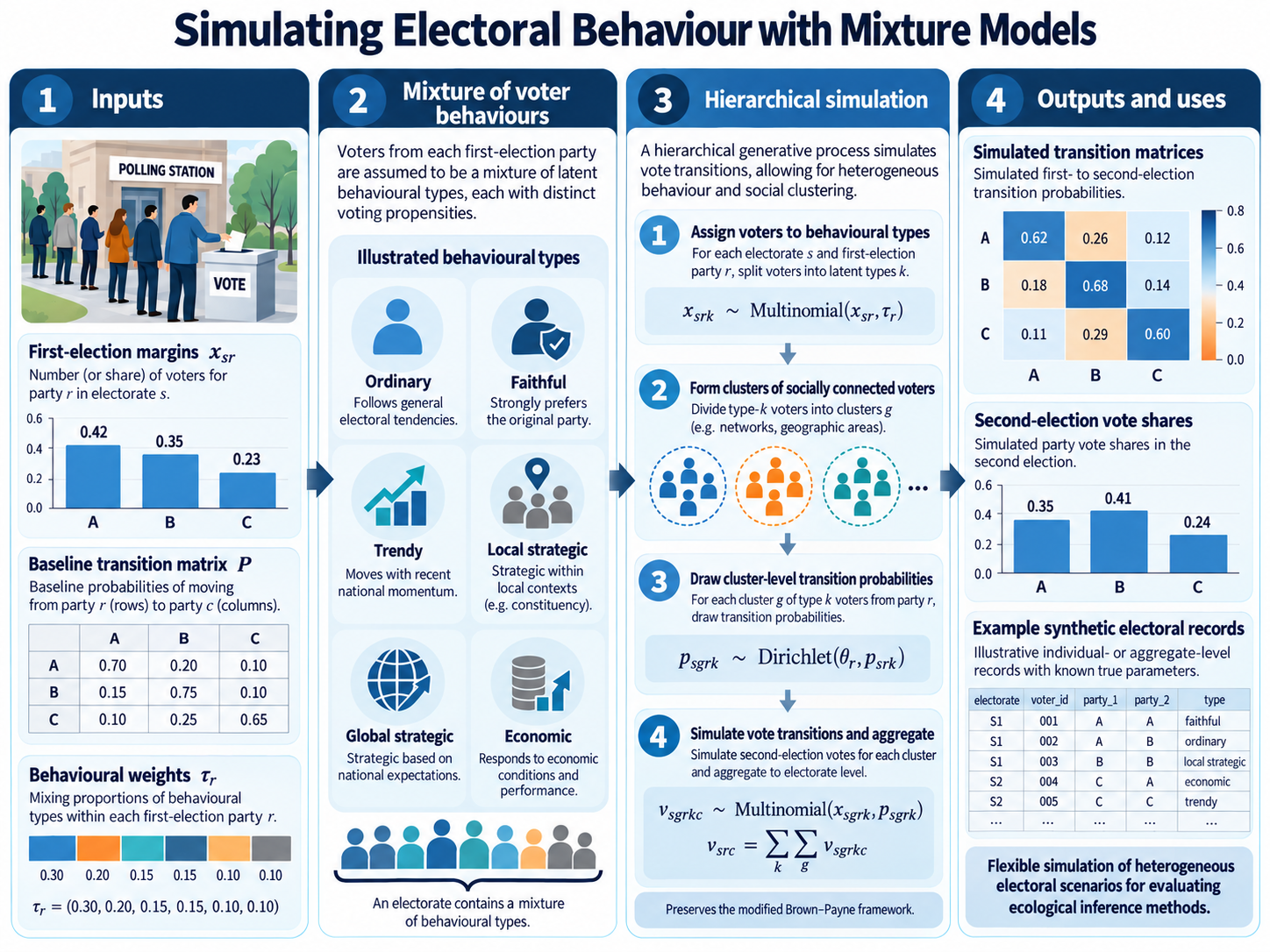
The algorithm implemented in the function simula_mixture extends this framework by first splitting the \(x_{sr}\) voters in each unit into behavioural types, then allocating them to clusters, and finally drawing cluster-level second-election counts from a Dirichlet–multinomial distribution with transition probabilities that depend on the unit, the first-election choice, and the behavioural type, before aggregating them to obtain unit-level outcomes.
3. A Mixture Framework for Electoral Behaviour
The simula_mixture function introduces two main extensions to the simulation framework previously introduced in 6. First, voter heterogeneity is represented through a mixture of behavioural types, which preserves the second-order moment structure of the model. Second, it allows for a larger set of behavioural types, increasing the range of possible voter behaviours.
Compared to the simula_BPF_with_deviations function 6, which assigns to each unit a single transition matrix obtained as a mixture of four voter types (ordinary, loyal, trending, and local strategic), the simula_mixture function allows distinct transition matrices for up to ten behavioural types. This flexibility implies a relatively rich set of function arguments, allowing for a high degree of user customisation. Details on the inputs and outputs of the function are provided in Appendix A.
Under this framework, voters at polling station \(s\) are assumed to belong to latent groups characterised by different preferences. The composition of these groups may vary across polling stations and may depend on the option chosen in the first election.
Following the standard mixture-model framework 16, voters are assumed to belong to latent types, and the numbers of voters of each type within a polling station are modelled using a multinomial distribution determined by user-specified probabilities. Since the likelihood of belonging to a given type may reasonably depend on the party supported in the previous election, we assume that the numbers of voters of the different types among those who voted for option \(r\) in the earlier election follow a multinomial distribution:
We consider up to ten behavioural types: ordinary, faithful, trendy, economic, and three types of strategic voters, with each strategic type having two variants. All strategic voter types are obtained by modifying the logits of the transition probabilities for ordinary voters through a strength-dependent adjustment term. Specifically,
-
Ordinary:
These voters behave according to the modified Brown–Payne model, with transition probabilities determined by the global baseline \(R\times C\) transition matrix \(\pmb{P} = [p_{rc}]\).
-
Faithful:
These are militants or voters strongly attached to a party who will vote for the same party again with probability close to one. Because competing parties may change across elections, the user provides a matrix \(\pmb{F}\) of transition probabilities for faithful voters. Most entries in each row will typically be zero, with the remaining ones summing to one. If the same voting options are available in the two elections, \(\pmb{F}\) will usually be the identity matrix.
-
Trendy:
These voters are assumed to have chosen party \(r\) in the first election only by chance, perhaps because it was in fashion or because they were following the advice of friends or relatives, without a stable attachment to that party. Their behaviour is determined by a vector \(\pmb{t}\) provided by the user, whose entries are non-negative and sum to one. Ordinarily, \(\pmb{t}\) is the vector of expected results in the second election implied by polls, or is derived from the matrix \(\pmb{P}\), assuming that all voters behave as ordinary voters.
Formally, these voters follow the matrix of transition probabilities \(\pmb{1}_R \pmb{t}\).
-
Local retrospective strategic:
The decisions of these voters depend on the local strength of the party they supported in the previous election. If their party was a minor one, they support it again when it appears sufficiently strong locally; otherwise they may switch to avoid wasting their vote. If their party was a major one, they support it again when it appears to need their support, otherwise they may feel free to choose differently. Transition probabilities are obtained by modifying the logits of the ordinary voters according to the local vote share \(\pi_{sr}\) relative to a threshold \(a_r\).
Formally, let \(\pmb{f}_r\) denote the \(r\)-th row of the matrix \(\pmb{F}\), and let \(\pmb{\lambda}_r\) denote the vector of logits \(\log(\pmb{p}_r/p_{rC})\) derived from the matrix of transition probabilities for ordinary voters (after deleting the last element, which is equal to zero). The vector of locally strategy-modified logits for polling station \(s\) is defined as
\begin{equation} \label{eq:4} \pmb{\lambda}^{LRS}_{sr} = \pmb{\lambda}_r + \beta_r\left(\pi_{sr}-a_r\right)\pmb{f}_r, \tag{4} \end{equation}where \(\pi_{sr}\) is the proportion of votes obtained by party \(r\) in polling station \(s\) in the first election and \(a_r\) is a threshold parameter. If \(\beta_r>0\), voters are more likely to support their party again when it appears sufficiently strong locally, whereas if \(\beta_r<0\) they become less likely to support the party when it appears too strong.
-
Global retrospective strategic:
These voters behave similarly to the previous type, but their decisions depend on the global electoral strength of the party they supported in the first election rather than on local results. Transition probabilities are obtained by modifying the logits of ordinary voters according to the global vote share \(\pi_r\) relative to a threshold \(b_r\).
Formally, the strategy-modified logits are defined as
\begin{equation} \label{eq:5} \pmb{\lambda}^{GRS}_{r} = \pmb{\lambda}_r + \gamma_r\left(\pi_r-b_r\right)\pmb{f}_r, \tag{5} \end{equation}where \(\pi_r\) denotes the overall vote share of party \(r\) in the first election and \(b_r\) is a threshold parameter.
-
Global strategic:
These voters base their decisions on the expected strength of parties in the second election. If the party they supported in the first election is expected to be sufficiently strong, they are more likely to support it again; otherwise they may switch strategically. Transition probabilities are obtained by modifying the logits of ordinary voters according to the expected second-election vote share \(\sum_j \pi_j p_{jr}\) relative to a threshold \(c_r\).
Formally, assuming that the order of parties coincides in the two elections for the relevant options, the strategy-modified logits are defined as
\begin{equation} \label{eq:6} \pmb{\lambda}^{GS}_{r} = \pmb{\lambda}_r + \varphi_r \left(\sum_j \pi_j p_{jr} - c_r\right) \pmb{f}_r, \tag{6} \end{equation}where \(\sum_j \pi_j p_{jr}\) represents the expected vote share of party \(r\) in the second election and \(c_r\) is a threshold parameter.
-
Economic:
These voters prioritise economic performance and reward or punish parties belonging to the governing coalition depending on the perceived change in the economic situation. Their behaviour modifies the logits of ordinary voters through a parameter linking economic variation in each voting unit with the parties belonging to the governing coalition.
Formally, let \(v_{s}\) denote the perceived measure of economic variation in unit \(s\) and \(\mathbf{g}\) a vector with entries equal to 1 for parties in the governing coalition and 0 otherwise. The vector of economically modified logits for unit \(s\) is then defined as
\begin{equation} \label{eq:7} \pmb{\lambda}_{sr}^{E} = \pmb{\lambda}_{r} + \alpha_{r}\,v_{s}\,\mathbf{g}, \tag{7} \end{equation}with \(\alpha_{r} > 0\) being a mapping parameter. Under this specification, these voters are more likely to support government parties when the local economy improves and punish them when it deteriorates.
Each behavioural group generates transition probabilities according to specific rules derived from the overdispersed multinomial model that modify baseline transition probabilities. This mixture structure allows the simulation of complex electoral scenarios in which multiple behavioural mechanisms coexist within the same electorate.
4. Comparison with Previous Simulation Functions
The simula_mixture function extends the simulation tools previously introduced in the eiCircles package 9, namely simula_BPF and simula_BPF_with_deviations 6. Although all three functions are grounded in the modified Brown–Payne framework, they differ in the way heterogeneity in voting behaviour is introduced.
The simula_BPF function generates artificial electoral data under the assumption that the transition probabilities between the two elections are homogeneous across polling units. In this case, all voters are assumed to follow the same set of baseline transition probabilities, while overdispersion arises only from the Dirichlet–multinomial structure associated with cluster-level interactions. In this sense, simula_BPF can therefore be viewed as a particular instance of simula_mixture when all the voters in all the units behave as ordinary voters.
The simula_BPF_with_deviations function relaxes this homogeneity assumption by allowing the transition probabilities to vary across polling units. In this framework, each unit-specific transition matrix is constructed as a weighted combination of several underlying transition mechanisms associated with different behavioural types, including loyal voters, trend-following voters, and contextually influenced voters.
The approach adopted in simula_mixture differs from that of the previous two functions in that behavioural heterogeneity is introduced directly at the level of individual voters rather than through unit-specific transition matrices. Instead of constructing a different transition table for each polling unit, the electorate is assumed to be composed of a mixture of latent behavioural types, each characterised by its own mechanism for generating transition probabilities. This modelling strategy provides greater flexibility in representing heterogeneous voting behaviour.
Because different behavioural types may coexist within the same polling unit, the resulting simulation framework can reproduce complex electoral environments where strategic behaviour, party loyalty, trend-following dynamics, and economic voting operate simultaneously.
In addition, the simula_mixture function removes several restrictions present in earlier simulation tools. In particular, it is not limited to square transition matrices and can therefore simulate elections in which the number of options differs between the two contests. Furthermore, the mixture structure typically produces datasets with greater variability in transition patterns, which may be particularly useful when evaluating the robustness of ecological inference methods.
5. Hierarchical Generative Model
In addition to providing greater flexibility in representing heterogeneous voting behaviour, the simulation mechanism implemented in simula_mixture can be interpreted, from a statistical viewpoint, as a hierarchical generative model that combines three sources of heterogeneity: behavioural heterogeneity, cluster-level correlation, and multinomial sampling variability.
For each polling unit \(s = 1,\dots,n\) and each option \(r\) in the first election, let \(x_{sr}\) denote the number of voters who supported option \(r\) in election 1. The simulation proceeds through the following hierarchical structure.
-
Behavioural heterogeneity:
Each voter belonging to group \(r\) is assigned, according to a multinomial distribution, to one of \(K\) behavioural types, which in turn behave according to a vector of transition probabilities \(\mathbf{p}_{srk}\) obtained by modifying the baseline transition probabilities \(\mathbf{p}_r\) through the behaviour-specific mechanisms described in Section 3. These mechanisms may depend on local electoral conditions, global electoral results, or contextual economic indicators.
-
Cluster-level heterogeneity:
Within each unit and behavioural group, voters are divided into clusters representing socially connected individuals. For each cluster \(g\), a vector of transition probabilities, \(\mathbf{p}_{sgrk}\), is drawn from a Dirichlet distribution centred on the behaviour-specific vector:
\begin{equation} \label{eq:8} \mathbf{p}_{sgrk} \sim \mathit{Dirichlet}\left(\theta_r, \mathbf{p}_{srk}\right), \tag{8} \end{equation}where \(\theta_r\) controls the degree of overdispersion around the baseline transition probabilities.
-
Individual vote transitions:
Conditional on the cluster-specific probability vector \(\mathbf{p}_{sgrk}\), the number of voters moving from option \(r\) in the first election to option \(c\) in the second election is generated from a multinomial distribution:
\begin{equation} \label{eq:9} \mathbf{v}_{sgrkc} \sim \mathit{Multinomial}\left(x_{sgrk}, \mathbf{p}_{sgrk}\right). \tag{9} \end{equation}Finally, transitions across clusters and behavioural types are aggregated to obtain the joint distribution of votes within each polling unit:
\begin{equation} \label{eq:10} v_{src} = \sum_{k} \sum_{g} v_{sgrkc}. \tag{10} \end{equation}This hierarchical structure combines three layers of stochastic variation: behavioural heterogeneity across voters, correlated decisions within social clusters, and individual-level randomness in voting decisions. As a result, the simulated datasets can reproduce a wide range of electoral dynamics commonly observed in empirical settings.
-
Generation of first-election
margins:
When the numbers of voters who supported option \(r\) in each polling unit \(s\) in election 1, \(x_{sr}\), are not provided, an additional layer of stochastic variation is introduced. In this case, the
simula_mixturefunction generates the vectors \(\mathbf{x}_s\) using a two-step procedure. Conditional on the unit size \(s_s = \sum_r x_{sr}\), a vector of expected probabilities \(\mathbf{r} = (r_1, \dots, r_R)\) for the options in election 1, and an overdispersion parameter \(\theta_r\), the process proceeds as follows. First, a probability vector \(\mathbf{r}_s\) is drawn from a Dirichlet distribution, \(\mathbf{r}_s \sim \mathit{Dirichlet}(\theta_r, \mathbf{r})\). Then, the vector of counts is generated from a multinomial distribution, \(\mathbf{x}_s \sim \mathit{Multinomial}(s_s, \mathbf{r}_s)\). Smaller values of \(\theta_r\) lead to greater variability across units, whereas larger values imply that the row-marginal unit-level proportions \(\mathbf{x}_s / s_s\) are closer to \(\mathbf{r}\).
6. Illustrative Simulation Examples
Previous sections introduce the statistical foundations of the simula_mixture function and the behavioural mechanisms embedded in the proposed simulation framework. While the mathematical formulations in Section 3 describe how each behavioural mechanism modifies individual transition probabilities, its practical implications are more clearly demonstrated through illustrative simulation examples. Accordingly, this section examines a set of representative simulation scenarios illustrating how variations in the behavioural composition of the electorate and in the parameters governing specific behavioural mechanisms systematically shape the resulting transition matrices and aggregate vote distributions.
The objective of these examples is not to replicate a specific empirical election but to evaluate, under controlled conditions, the contribution of each behavioural mechanism to the simulated electoral dynamics. To facilitate meaningful cross-scenario comparisons, all simulation parameters remain fixed except for the specific behavioural mechanism under evaluation. Consequently, any observed variations can be directly attributed to the behavioural assumptions embedded within the model. The selected scenarios correspond to the principal behavioural mechanisms introduced in Section 3, defining stylised electoral configurations that align with empirical patterns documented in the electoral literature.
Throughout this section, the baseline transition matrix for ordinary voters is set to
The simulated electoral system therefore consists of three competing parties. Additionally, we set the number of polling stations to 100, simulate polling-station sizes from a uniform distribution between 300 and 800, fix the expected first-election vote shares equal to (0.30, 0.45, 0.25), and consider the default values of the dispersion parameters implemented in the package (see Table 1 for details). Unless otherwise stated, each scenario is evaluated 100 times, using 100 independent replicates, and the reported transition matrices and second-election vote distributions correspond to the averages obtained across those experimental runs.
| Parameter | Value |
| Parties | 3 |
| Polling stations | 100 |
| Polling size (voters) | Uniform \((300,800)\) |
| 1st election vote shares | \((0.30,0.45,0.25)\) |
| \(\theta_1,\theta_2\) | Default values |
| \(\xi\) | Default value |
| Baseline matrix | Eq. (11) |
| Replicates | 100 |
6.1. Baseline Simulation with Ordinary Voters
The first scenario considers the configuration in which all individuals are assumed to behave as ordinary voters. Under this scenario, transition probabilities are governed exclusively by the baseline transition matrix defined previously, without the additional behavioural adjustments introduced by the remaining voter types (Section 3). This scenario therefore serves as a control benchmark against which the subsequent effects of alternative behavioural mechanisms can be evaluated.
Figure 1 compares the baseline transition matrix specified as an input to simula_mixture with the average transition matrix obtained from 100 independent simulation replicates.
The simulated transition probabilities closely reproduce the baseline values, indicating that the simulation algorithm accurately preserves the expected transition structure while incorporating the stochastic variability induced by the hierarchical Dirichlet–multinomial model. The small differences between the input and model-derived matrices are entirely consistent with the random variation inherent to the simulation process. They provide empirical evidence that the implementation correctly reproduces the theoretical behaviour of the baseline model.
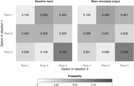
Fig. 1. Baseline transition matrix supplied to simula_mixture (left) and average transition matrix obtained from 100 independent simulation replicates assuming ordinary voting behaviour only (right).
6.2. Effect of Alternative Behavioural Mechanisms
The behavioural mechanisms introduced in Section 3 are illustrated through six representative simulation scenarios under a common baseline electoral setting. The first five scenarios isolate the effects of individual behavioural mechanisms and comprise: (i) ordinary voters only; (ii) mixtures of ordinary and faithful voters; (iii) mixtures of ordinary and trendy voters; (iv) mixtures of ordinary and local retrospective strategic voters; and (v) mixtures of ordinary and economically motivated voters. The sixth scenario combines several behavioural mechanisms simultaneously within the same electorate, illustrating one of the principal methodological features of simula_mixture.
For each of the four pairwise mixed scenarios, ordinary voters represent \(50\%\), \(80\%\), and \(20\%\) of the previous supporters of Parties 1, 2, and 3, respectively. The remaining voters are assigned to the behavioural mechanism under consideration. These proportions are kept identical across scenarios so that any observed differences can be attributed exclusively to the behavioural mechanism being introduced. The baseline transition matrix, first-election vote shares, polling-station sizes, dispersion parameters, and all remaining simulation settings remain unchanged (see Table 1).
The combined-mixture scenario adopts the same behavioural composition for the previous supporters of every first-election party: \(30\%\) ordinary voters, \(30\%\) faithful voters, \(20\%\) trendy voters, and \(20\%\) economically motivated voters. This configuration is intentionally illustrative and is included to demonstrate the flexibility of the proposed framework rather than to represent a particular electoral setting.
Figure 2 presents the average transition matrices obtained from 100 independent simulation replicates under the six behavioural configurations, while Table 4 (in Appendix A) provides an example of the simula_mixture call used in each scenario.
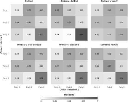
Fig. 2. Average transition matrices obtained under six illustrative behavioural configurations. The first five scenarios isolate the effects of individual behavioural mechanisms. The final scenario illustrates the simultaneous coexistence of four behavioural types within the same electorate (30% ordinary, 30% faithful, 20% trendy, and 20% economically motivated voters for each first-election party). All matrices correspond to the average of 100 independent simulation replicates and are displayed using a common colour scale.
Faithful voters use the identity matrix as their transition matrix, thereby remaining with the party supported in the first election. Consequently, the diagonal entries of the aggregate transition matrix increase, reflecting stronger party loyalty and lower electoral mobility. As expected from the specified mixture proportions, the strongest reinforcement of the diagonal is observed for Party 3, whose previous supporters include the largest proportion (\(80\%\)) of faithful voters. This stylised mechanism represents persistent party attachment, one of the most widely recognised regularities in electoral behaviour.
Trendy voters follow a common second-election probability vector rather than transition probabilities conditional on their first-election choice. In the present illustration, this common probability vector is obtained from the expected second-election vote distribution implied by the baseline transition matrix. As a result, the rows of the transition matrix become more homogeneous, reducing the dependence between voting choices across the two elections. This provides a stylised representation of trend-following behaviour, whereby voting decisions are influenced by the expected aggregate electoral outcome rather than by previous partisan preferences.
Local retrospective strategic voters modify their transition probabilities according to the adjustment defined in Eq. (4), which depends on the local electoral strength of the party they supported in the first election together with the corresponding threshold and elasticity parameters. In the simulations, Party 3 is treated as a minor party, with parameters \(a_3 = 0.2\) and \(\beta_3 = 1.2\), whereas Parties 1 and 2 are treated as major parties, with parameters \(a_1 = 0.5\), \(a_2 = 0.6\), \(\beta_1 = -0.1\), and \(\beta_2 = -0.2\) (see Table 4 in Appendix A for details of how these parameter values are specified in the calls to simula_mixture). The resulting aggregate transition matrix reflects the interaction between the specified strategic parameters and the heterogeneous electoral composition of individual polling stations. This scenario provides a stylised representation of context-dependent voting behaviour, consistent with the importance of local electoral environments documented in the electoral behaviour literature 13,14.
Economically motivated voters modify their transition probabilities through the adjustment defined in Eq. (7), which combines the local economic conditions with the parties belonging to the governing coalition. In the present illustration, Party 1 is assumed to be the sole governing party, with the variation in economic performance across polling stations following a uniform distribution between \(-1\) and \(1\) (see Table 4 in Appendix A for details of how this is specified in the calls to simula_mixture). The same vector of local economic conditions is used in all replicates, so that differences between them are attributable solely to the stochastic variation rather than to changes in the simulated economic environment. Moreover, the positive sensitivity parameters adopted in the simulation (\(\alpha_1 = 1.1\), \(\alpha_2 = 0.9\), and \(\alpha_3 = 0.6\)) imply that favourable economic conditions increase the probability of transitions towards Party 1, whereas adverse conditions decrease it. The larger value of \(\alpha_1\) makes former Party 1 voters more responsive to local economic conditions than voters of the other parties. This mechanism provides a stylised representation of economically motivated voting by linking local economic conditions with support for the governing party/coalition, consistent with the reward–punishment mechanisms discussed in the economic voting literature 17.
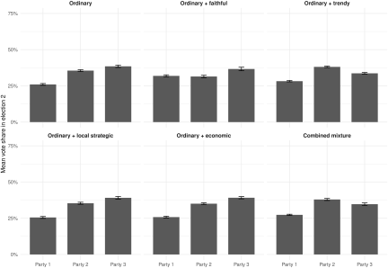
Fig. 3. Average second-election vote distributions obtained under the six illustrative behavioural configurations. Error bars denote one standard deviation across the 100 simulation replicates.
The final scenario combines faithful, trendy, and economically motivated voters within the same electorate (see Table 4 in Appendix A). Unlike the previous examples, which isolate individual mechanisms for interpretability, this scenario demonstrates the full flexibility of simula_mixture. Different behavioural types coexist within each first-election group and jointly determine the aggregate transition structure. The resulting transition matrix therefore captures the interaction between several behavioural processes, producing electoral patterns that cannot be generated by any single mechanism in isolation.
Figure 3 shows how the structural differences observed in the transition matrices translate into distinct aggregate vote distributions in the second election. Although all six scenarios share the same baseline transition matrix and first-election vote shares, their aggregate electoral outcomes differ because each behavioural composition modifies the underlying transition probabilities differently.
The comparison is particularly relevant for ecological inference, which is generally based on observed electoral margins rather than on the latent transition matrix itself. The examples demonstrate that alternative behavioural assumptions—including scenarios in which multiple mechanisms operate simultaneously—can generate clearly distinguishable aggregate electoral outcomes despite sharing a common baseline electoral setting.
6.3. Sensitivity to the Intensity of Strategic Voting
The previous subsection examines the effect of changing the behavioural composition of the electorate. A complementary analysis consists of assessing how the simulated electoral outcomes vary when the intensity of a given behavioural mechanism is modified while all other model components remain unchanged. To illustrate this capability, a sensitivity analysis is conducted for the local retrospective strategic voting mechanism.
The analysis considers three levels of strategic intensity by varying the elasticity parameters in the adjustment defined in Eq. (4). In the first scenario, the elasticity parameters are set equal to zero, so that no strategic adjustment is applied. The second scenario uses the baseline elasticity parameters adopted in the illustrative example. Finally, the third scenario multiplies those parameters by three, representing a substantially stronger response to local electoral conditions. All remaining simulation inputs, including the mixture proportions, threshold parameters, and baseline transition matrix, are kept unchanged.
Figure 4 presents the average transition matrices obtained under the three levels of strategic intensity. When the elasticity parameters are equal to zero, voters assigned to the local retrospective strategic category behave almost identically to ordinary voters because no strategic adjustment is introduced. As the elasticity parameters increase, the transition probabilities progressively depart from the baseline configuration, illustrating the increasing influence of local electoral conditions on individual voting behaviour.
The direction and magnitude of these changes depend jointly on the signs of the elasticity parameters, the local first-election vote shares, and the corresponding threshold values. Consequently, the parameters of simula_mixture do not merely determine the presence or absence of a behavioural mechanism but also provide continuous control over its influence on the simulated electorate.
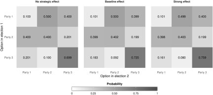
Fig. 4. Average transition matrices obtained under three levels of local retrospective strategic voting. From left to right: no strategic adjustment, baseline elasticity parameters, and elasticity parameters multiplied by three.
Figure 5 shows the corresponding second-election vote distributions. The progressive differences between the three scenarios demonstrate how modifications introduced at the level of individual transition probabilities propagate to observable aggregate electoral outcomes. This example illustrates the usefulness of simula_mixture for constructing controlled simulation experiments in which the strength of a specific behavioural mechanism can be varied systematically while all other components of the model remain fixed.
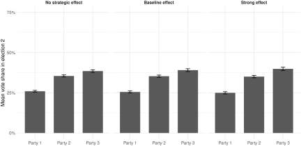
Fig. 5. Average second-election vote distributions under three levels of local retrospective strategic voting. Error bars denote one standard deviation across the 100 simulation replicates.
6.4. Variability Across Simulation Replicates
The previous examples compare the effects of different behavioural mechanisms under identical simulation settings. It is also useful to assess the Monte Carlo variability introduced by the stochastic simulation procedure itself. Table 2 reports, for each behavioural scenario, the average cell-specific standard deviation of the simulated transition probabilities together with the average standard deviation of the second-election vote shares across the 100 simulation replicates.
These quantities measure the variability generated by the simulation procedure itself rather than the sampling uncertainty associated with an empirical estimator. Their inclusion makes it possible to distinguish differences attributable to the behavioural mechanisms from those arising solely from stochastic simulation.
| Scenario |
Mean cell SD |
Mean vote SD |
| Ordinary | 0.007 | 0.007 |
| Faithful | 0.005 | 0.009 |
| Trendy | 0.008 | 0.005 |
| Local strategic | 0.007 | 0.007 |
| Economic | 0.007 | 0.007 |
| Combined | 0.006 | 0.007 |
The reported standard deviations remain consistently small across all six behavioural scenarios. The combined-mixture scenario exhibits a level of Monte Carlo variability comparable to those observed for the individual behavioural mechanisms, indicating that allowing several behavioural types to coexist does not introduce substantial additional stochastic variability into the simulation process.
Overall, these results indicate that the differences observed in the transition matrices and aggregate vote distributions are primarily driven by the behavioural mechanisms incorporated into the simulation model rather than by Monte Carlo variability.
Taken together, the illustrative examples demonstrate that simula_mixture can generate markedly different electoral transition structures and aggregate vote distributions from a common baseline electoral setting through controlled modifications of either the behavioural composition of the electorate or the intensity of individual behavioural mechanisms. They also show that the proposed framework naturally accommodates scenarios in which several behavioural mechanisms operate simultaneously within the same electorate, thereby providing a flexible and reproducible simulation environment for methodological studies in ecological inference.
7. Conclusions
This paper introduces simula_mixture, a new simulation function implemented in the R package eiCircles for generating artificial electoral data under a flexible mixture of voter behaviours within the framework of the overdispersed multinomial model.
The proposed framework allows up to ten behavioural mechanisms to coexist within the same electorate, thereby providing a flexible tool for constructing synthetic electoral datasets with heterogeneous transition structures. By combining different behavioural mechanisms and adjusting their relative proportions or intensities, the simulator can reproduce a broad range of stylised electoral scenarios within a common modelling framework.
The illustrative examples presented in this paper demonstrate how alternative behavioural assumptions lead to markedly different transition matrices and aggregate vote distributions while all other simulation settings remain unchanged. They also show that the influence of individual behavioural mechanisms can be controlled continuously through their associated model parameters, providing a transparent framework for designing reproducible simulation experiments.
These characteristics make simula_mixture particularly useful for benchmarking ecological inference methods, investigating the effects of behavioural heterogeneity on electoral outcomes, studying the consequences of strategic or economically motivated voting, and generating synthetic electoral data for methodological research and teaching.
Future research may extend the framework by incorporating additional behavioural mechanisms, considering interactions between existing mechanisms, or simulating electoral transitions across more than two elections.
Acknowledgments
The authors are deeply grateful to Antonio Forcina for his invaluable contributions to the conception, design, and implementation of simula_mixture, as well as for his insightful comments and constructive suggestions throughout the development of this work. The authors would also like to express their sincere gratitude to the Editor and the anonymous reviewers for their careful evaluation of the manuscript and for their insightful comments and constructive suggestions, which have significantly contributed to improving the clarity, quality, and overall presentation of the work. Any remaining errors or omissions are solely the responsibility of the authors. This research was supported by the Generalitat Valènciana, Conselleria de Educación, Cultura y Universidades (grant CIACO/2023/031); the MCIN/AEI/10.13039/501100011033 and the European Regional Development Fund (ERDF) (grant PID2022-139469NB-I00); the Junta de Castilla y León and the European Regional Development Fund (ERDF) (grant CLU-2025-2-03); and Fundación Ramón Areces (grant CISP18A6216). The funding bodies had no role in the study design; the collection, analysis, or interpretation of the data; the writing of the manuscript; or the decision to submit the paper for publication.
- [1] J. M. Pavía and R. Romero, “Symmetry estimating R×C vote transfer matrices from aggregate data,” J. of the Royal Statistical Society, Series A – Statistics in Society, Vol.187, No.4, pp. 919-943, 2024. https://doi.org/10.1093/jrsssa/qnae013
- [2] J. M. Pavía, P. Pérez-Asurmendi, and R. de Andrés Calle, “Ecological inference for electoral analysis: A computational perspective on human decision-making,” V. Torra, Y. Narukawa, and J. Domingo-Ferrer (Eds.), “Modeling Decisions for Artificial Intelligence, MDAI 2025, Lecture Notes in Computer Science, Vol.15957,” Springer, pp. 15-26, 2026. https://doi.org/10.1007/978-3-032-00891-6_2
- [3] T. Abou-Chadi and L. Stoetzer, “How parties react to voter transitions,” American Political Science Review, Vol.114, No.3, pp. 940-945, 2020. https://doi.org/10.1017/S0003055420000155
- [4] A. Penadés and J. M. Pavía, “An ecological inference approach to the origins of proportional representation,” Social Science Information, Vol.63, No.2, pp. 168-192, 2024. https://doi.org/10.1177/05390184241250179
- [5] A. Klima, P. W. Thurner, C. Molnar, T. Schlesinger, and H. Küchenhoff, “Estimation of voter transitions based on ecological inference: An empirical assessment of different approaches,” AStA-Advances in Statistical Analysis, Vol.100, No.2, pp. 133-159, 2016. https://doi.org/10.1007/s10182-015-0254-8
- [6] J. M. Pavía and A. Forcina, “Simulating electoral behavior,” V. Torra, Y. Narukawa, and J. Domingo-Ferrer (Eds.), “Modeling Decisions for Artificial Intelligence, MDAI 2025, Lecture Notes in Computer Science, Vol.15957,” Springer, pp. 54-65, 2026. https://doi.org/10.1007/978-3-032-00891-6_5
- [7] M. Barreto, L. Collingwood, S. Garcia-Rios, and K. A. R. Oskooii, “Estimating candidate support in voting rights act cases: Comparing iterative EI and EI-R_C methods,” Sociological Methods & Research, Vol.51, No.1, pp. 271-304, 2022. https://doi.org/10.1177/0049124119852394
- [8] J. M. Pavía and R. Romero, “Improving estimates accuracy of voter transitions. Two new algorithms for ecological inference based on linear programming,” Sociological Methods & Research, Vol.53, No.4, pp. 1491-1533, 2024. https://doi.org/10.1177/00491241221092725
- [9] A. Forcina and J. M. Pavía, “eiCircles: Ecological Inference of RxC Tables by Overdispersed-Multinomial Models,” R-package, version 0.0.1-14, CRAN, 2026. https://doi.org/10.32614/CRAN.package.eiCircles
- [10] A. Forcina, M. Gnaldi, and B. Bracalente, “A revised Brown and Payne model of voting behaviour applied to the 2009 elections in Italy,” Statistical Methods & Applications, Vol.21, pp. 109-119, 2012. https://doi.org/10.1007/s10260-011-0184-x
- [11] P. J. Brown and C. D. Payne, “Aggregate data, ecological regression, and voting transitions,” J. of the American Statistical Association, Vol.81, No.394, pp. 452-460, 1986. https://doi.org/10.2307/2289235
- [12] A. Forcina and J. M. Pavía, “From Corrado Gini’s early contributions to overdispersion to modern models of voting behaviour,” Statistical Science, Vol.11, No.1, pp. 201-210, 2026. https://doi.org/10.1214/24-STS960
- [13] C. Pattie and R. Johnston, “‘People who talk together vote together’: An exploration of contextual effects in Great Britain,” Annals of the Association of American Geographers, Vol.90, No.1, pp. 41-66, 2000. https://doi.org/10.1111/0004-5608.00183
- [14] H. Schmitt, P. Segatti, and C. van der Ejik, “Consequences of Context: How Social, Political and Economic Environments Affect Voting,” ECPR Press, 2021.
- [15] A. Forcina and J. M. Pavía, “Estimating vote transition counts in Ecological Inference,” Statistics and Public Policy, Vol.13, No.2654396, 2026. https://doi.org/10.1080/2330443X.2026.2654396
- [16] G. J. McLachlan and D. Peel, “Finite Mixture Models,” Wiley, 2000.
- [17] M. S. Lewis-Beck and M. Paldam, “Economic voting: an introduction” Electoral Studies, Vol.19, Nos.2-3, pp. 113-121, 2000. https://doi.org/10.1016/S0261-3794(99)00042-6
Appendix
Appendix A. The simula_mixture Function
This appendix provides a schematic overview of the implementation of the simula_mixture function. Table 3 summarises its main arguments, while Table 4 demonstrates their practical use. For a complete description of simula_mixture arguments see the package documentation 9, including both the required inputs and the principal optional arguments (theta1, theta2, cs, TP.f, TP.t, LRSV.par, GRSV.par, GSV.par, and eco.par). Table 3 complements the methodological description presented in the main text and clarifies how the different components of the simulation framework can be specified. The structure of the outputs returned by the function is also described.
As its main outputs, the function provides a three-dimensional \(R \times C \times n\) array containing the simulated vote counts \(\{v_{src}\}\), with index \(s\) running along the third dimension, together with its three marginal two-dimensional distributions: the \(R \times C\) matrix of global vote counts, \([v_{rc}=\sum_{s} v_{src}]\); the \(n \times R\) matrix, \([x_{sr}=\sum_{c} v_{src}]\), containing the vote distributions in Election 1; and the \(n \times C\) matrix, \([y_{sc}=\sum_{r} v_{src}]\), containing the vote distributions in Election 2. Note that, in real elections, the first matrix is usually unobserved, whereas the latter two matrices constitute the inputs to ecological inference models.
While Table 3 summarises the main inputs of simula_mixture, Table 4 demonstrates their practical use by reproducing the basic calls made for each replicate in the scenarios analysed in Section 6.2. The examples present the basic workflow required to generate a simulated election. The returned object contains the complete set of simulated electoral outcomes, whose main components are described above. Starting from the baseline setup (General Specifications), adjustments to the behavioural composition matrix (tau) regulate the voter types within the electorate to reproduce different voting dynamics, while the LRSV.par and eco.par arguments control how the local strategic and economic voters behave in the scenarios simulated. Default options are used for the faithful and trendy voters. More complex behavioural configurations can be implemented through the additional optional arguments.
| Argument | Description |
n.units |
The number of units \(n\) in which the electorate is divided. |
TP |
The row-standardized \(R\times C\) matrix with the underlying baseline global transition probabilities for ordinary voters: \(\boldsymbol{P} = [\boldsymbol{p}'_{1},\dots,\boldsymbol{p}'_{i},\dots,\boldsymbol{p}'_{R}]'\) |
prop1 |
The vector with the initial assumed probabilities of voting for each of the \(R\) competing options in the first election: \(\boldsymbol{r} = (r_1, \dots, r_i, \dots, r_R)\). |
polling.sizes |
Either a vector of two components with two positive integer numbers indicating the minimum and maximum number of voters for each unit or a vector of length \(n\) of positive integers specifying the number of voters in each unit: \((s_1, \dots, s_s, \dots, s_n)\). |
theta1 |
A number between 0 and 1 to be used as overdispersion parameter in election 1: \(\theta_r\). Default, \(0.1\). |
theta2 |
Either a single overdispersion parameter, \(\theta\), or a vector of length \(R\) containing overdispersion parameters \((\theta_1, \dots, \theta_r, \dots,\theta_R)\) to be used in the Dirichlet distributions of election 2. When this argument is a single number, \(\theta_r = \theta, \forall r\). Default, \(0.1\). |
cs |
A positive number indicating the average number of cluster size, \(\xi\). Default, \(50\). |
tau |
An \(R \times 7\) row-standardized matrix with the probabilities of each behavioural type conditional on the first-election option. Each entry \(\tau_{rk}\) gives the probability that a voter who chose option \(r\) behaves as type \(k\). |
TP.f |
An \(R \times C\) row-standardized matrix of transition probabilities for faithful voters, \(\pmb{F}\), typically close to the identity matrix. |
TP.t |
A vector of length \(C\) defining the transition probabilities for trendy voters, \(\pmb{t}\). By default, it reflects the expected second-election results. |
LRSV.par |
A \(4 \times R\) matrix of parameters, \([a'_{-}, \beta'_{-}, a'_{+},\beta'_{+}]'\), governing local retrospective strategic voting, based on past results within each unit. \(\beta_{-}=(\beta_1^{-}, \dots,\beta_R^{-})\) and \(\beta_{+}=(\beta_1^{+}, \dots,\beta_R^{+})\) are the elasticity parameters of minor-party and major-party voters, respectively, and \(a_{-}=(a_1^{-}, \dots, a_R^{-})\) and \(a_{+}=(a_1^{+}, \dots, a_R^{+})\) the corresponding thresholds. |
GRSV.par |
A \(4 \times R\) matrix of parameters, \([b'_{-},\gamma'_{-},b'_{+},\gamma'_{+}]'\), governing global retrospective strategic voting, based on aggregate past results. \(\gamma_{-}=(\gamma_1^{-}, \dots,\gamma_R^{-})\) and \(\gamma_{+}=(\gamma_1^{+}, \dots,\gamma_R^{+})\) are the elasticity parameters of minor-party and major-party voters, respectively, and \(b_{-}=(b_1^{-}, \dots, b_R^{-})\) and \(b_{+}=(b_1^{+}, \dots, b_R^{+})\) the corresponding thresholds. |
GSV.par |
A \(4 \times \min(R,C)\) matrix of parameters, \([c'_{-},\varphi'_{-},c'_{+},\varphi'_{+}]'\), governing forward-looking (global) strategic voting based on expected results. \(\varphi_{-}=(\varphi_1^{-}, \dots,\varphi_L^{-})\) and \(\varphi_{+}=(\varphi_1^{+}, \dots,\varphi_L^{+})\) are the elasticity parameters of minor-party and major-party voters, respectively, and \(c_{-}=(c_1^{-}, \dots, s_L^{-})\) and \(c_{+}=(c_1^{+}, \dots, c_L^{+})\) the corresponding thresholds, with \(L = \min(R,C)\). |
eco.par |
A list of parameters governing economic voting, including local economic variation, \([v_1,\dots, v_n]\), party-specific sensitivities, \([\alpha_1, \dots, \alpha_R]\), and government participation indicators, \(\textbf{g}\). |
simula_mixture for the considered behavioural scenarios.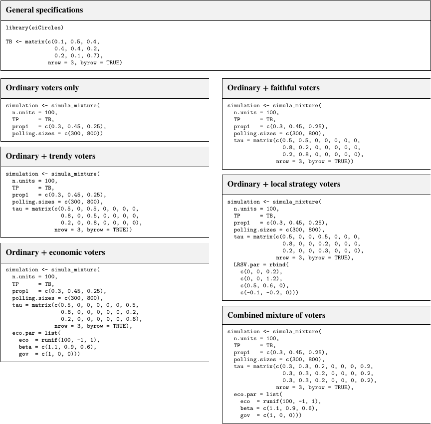
This article is published under a Creative Commons Attribution-NoDerivatives 4.0 Internationa License.