
Research Paper:
High-Speed Railway Train Delay Prediction Based on Improved CTGAN Generative Data Fusion
Qingyun Fu*,**
 , Tao Zhang*,**
, Shuxin Ding*,**,†
, Yanhao Sun*,**
, and Zhiming Yuan*,**
*Signal and Communication Research Institute, China Academy of Railway Sciences Co., Ltd.
No.2 Daliushu Road, Haidian District, Beijing 100081, China
**Traffic Management Laboratory for High-Speed Railway, National Engineering Research Center of System Technology for High-Speed Railway and Urban Rail Transit, China Academy of Railway Sciences Co., Ltd.
No.2 Daliushu Road, Haidian District, Beijing 100081, China
†Corresponding author

To address the issues of imbalanced and insufficient delay samples in training datasets for high-speed railway (HSR) delay prediction, this study proposes an HSR train delay prediction method based on improved Conditional Tabular Generative Adversarial Network (CTGAN) data fusion. This method employs an enhanced CTGAN for delay data generation, in which a transformer is integrated into the generator to better capture the spatiotemporal correlation features constructed from train operation scenarios. The quality of the generated delay data was rigorously analyzed using statistical and distribution similarity metrics, thereby validating the rationality of fusing the generated samples with the original data. Subsequently, a training delay prediction model based on CBLA (CNN-BiLSTM-Attention) was constructed and trained on the augmented dataset derived from data fusion. The output performance of the trained model was tested, and the optimal data fusion ratio was determined. Experimental results demonstrate that incorporating CTGAN-generated data significantly enhances the prediction accuracy. Specifically, when the generated data were fused at an optimal ratio of 4:1, the mean absolute error was reduced by approximately 38% and the root mean square error by approximately 78%.
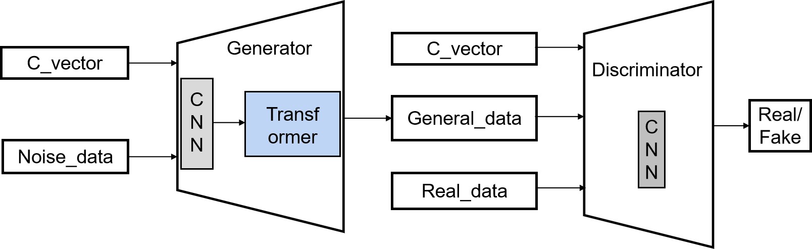
The overall network architecture of the transformer-enhanced CTGAN
1. Introduction
As an important development direction for railway dispatching and command equipment 1, an intelligent centralized traffic control system relies on relevant artificial intelligence technologies and algorithms to enhance its capabilities in auxiliary decision-making, delay prediction, and emergency response 2. With the rapid development of high-speed railways, the application of train operation data has become increasingly widespread 3. The continuous upgrading and optimization of train dispatching systems have enabled the collection and storage of massive amounts of train operation data 4. As important operational data, train delay data are of significant value for train operation analysis, dispatch optimization, and service quality improvement 5. However, in actual operation, trains usually run on time and delay data are relatively scarce; in particular, large delay data are even rarer. This scarcity severely limits the performance improvement of data-driven train delay analysis and related applications. Previous studies have typically adopted the following methods to address the scarcity of train delay data.
A traditional method for generating delay data involves simulating delays under different operational scenarios by constructing train operation simulation models. Considerable research has been devoted to developing simulation methods for analyzing train operations in large and complex railway networks 6,7,8,9, predicting train punctuality, and estimating delays 10,11. However, although simulation models provide a means of generating large amounts of data in a virtual environment, the difficulty of accurately modeling complex operational environments makes it challenging to ensure the fidelity of the generated data, thereby limiting their application in generating high-fidelity train-delay data. In addition, traditional statistical methods, such as using Gaussian mixture models and hidden Markov models, generate synthetic data by learning the distribution of delay data. However, these methods have limited ability to model high-dimensional, complex data distributions, resulting in low-quality generated data that fail to capture the complex nonlinear relationships and long-tailed characteristics of train-delay data.
In addition to studies addressing the lack of train delay data, various data-generation techniques have been explored for other railway applications to address data scarcity. For example, some studies have proposed methods for generating power current time-series data to monitor the status of railway switches 12. To address the shortage of defective fastener data in railway infrastructure inspection, researchers have generated synthetic image data using techniques such as style transfer to assist in defect detection 13. In addition, simulation frameworks such as TrainSim 14 have been used to generate LiDAR and camera datasets, providing large-scale labeled data for testing novel algorithms and training deep neural networks. Synthetic data have also been applied to construct digital twins of railway signals 15 and to improve the semantic segmentation accuracy of railway infrastructure using data generated from virtual models 16. Although successful in their respective application scenarios, these approaches have mainly focused on generating images, specific sensor data, or particular types of time-series data. They have also primarily emphasized data augmentation rather than generating complete sequences of train delay events with complex spatiotemporal correlations from scratch.
In recent years, generative adversarial networks (GANs) 17, first proposed by Goodfellow et al., have achieved remarkable results as powerful deep generative models in image and text generation. GANs can learn complex distributions of real data and generate high-quality synthetic data. For tabular data generation, Xu et al. proposed the Tabular GAN 18 and subsequently developed the conditional tabular generative adversarial network (CTGAN) 19. CTGAN is specifically designed for tabular data and can efficiently capture the mixed distributions of discrete and continuous variables. CTGAN has been successfully applied to address data imbalance problems and generate high-quality synthetic data, such as photorealistic data for balancing fault categories in power transformer dissolved gas analysis data augmentation 20, and feature generation to improve predictive model performance in the early detection of lung cancer 21. In addition, studies have proposed EID-GAN for processing extremely imbalanced data 22 and Anomaly-GAN for data augmentation in surface anomaly detection 23. However, train delay data are not merely tabular data, but also exhibit time-series characteristics and are subject to complex operational scenario constraints with intricate spatiotemporal correlations. Moreover, the generator in the traditional CTGAN mainly relies on convolutional neural networks (CNNs), which may have limited capability to capture long-range dependencies and complex relationships within complex spatiotemporal data sequences.
Based on the above background, this study aims to overcome the shortcomings of existing train delay data generation methods. We propose a train-delay data generation method based on an improved CTGAN. By optimizing the generator network architecture, the proposed method is designed to better capture the temporal and operational scenario characteristics of train delay data. It aims to generate high-quality synthetic train delay data that reflect diverse operational scenarios. This approach effectively addresses the issue of limited train delay data and offers robust support for subsequent data-driven applications, including train operation analysis, delay prediction, and scheduling optimization.
The remainder of this paper is organized as follows. Section 2 describes the improved CTGAN model proposed in this study. Section 3 presents the dataset and data processing methods. Section 4 presents the generation and evaluation of the delay data. Section 5 presents and analyzes the experimental results of the train delay prediction to validate the proposed methodology. Finally, Section 6 summarizes the study.
2. Model Construction
2.1. Network Architecture of Improved CTGAN
To create an improved CTGAN model, a transformer structure was added to the traditional CNN discriminator network of the generative adversarial CTGAN model. By leveraging the self-attention mechanism of the transformer, the model can better capture the spatiotemporal correlations between continuous variables (station delay times) and discrete variables (scenario features) in the train delay data. The improved generator network is responsible for generating delay data, whereas the discriminator network differentiates real from generated data. This adversarial collaboration between the generator and discriminator drives the generated data to progressively approximate the real data.
The transformer primarily comprises input embedding, positional encoding, an encoder, and output layers.
The input-embedding layer converts discrete input data into a continuous vector representation. The positional encoding layer is usually generated using sine and cosine functions so that the model can learn the relative positional information, and positional and dimension-specific encoding is implemented according to Eqs. (1) and (2):
The encoder processes an input sequence and transforms it into a series of representations containing contextual information. An encoder typically comprises a stack of \(N\) identical encoder layers. Each positional encoder consists of two main sublayers: a multi-headed self-attention network and a feed-forward network.
The multi-head attention mechanism is central to the encoder. The key to implementing the multi-head attention mechanism is the scaled dot product attention, whose input is a collection of three vectors: query vector (\(Q\)), key vector (\(K\)), and value vector (\(V\)).
The input query vector \(Q\), key vector \(K\), and value vector \(V\) are projected to different low-dimensional spaces by different linear transformations, that is, multiplying by different weight matrices \(W_i^Q\), \(W_i^K\), and \(W_i^V\) to form multiple pairs \((Q_{i}, K_{i}, V_{i})\), and the pairs \((Q_{i}, K_{i}, V_{i})\) of each group have the following linear transformation formulas in Eqs. (3), (4), and (5).
For each set \((Q_{i}, K_{i}, V_{i})\), the scaled dot product attention computation was performed independently. The specific computational procedure for the scaled click attention mechanism is given in Eqs. (6) and (7).
According to Eq. (6), if \(Q\) is a matrix representing its query for more than one piece of information, and \(K\) is a matrix representing the matching feature information with more than one element, the result \(\textit{Scores}\) is a matrix representing the matching feature information with more than one element, where element (\(i\), \(j\)) is the dot product of \(Q_i\) and \(K_j\), and each row of this matrix represents the similarity scores of a query for all the keys.
Equation (7) shows the process of calculating the attention weights, where \(d_k\) is the split sub-dimension allocated to each individual attention head, with a value of 64. The dot product result is scaled by dividing it by the square root of the key \(\sqrt{d_{k}}\), to prevent the dot product from being too large and causing the gradient of the softmax function to become very small. Softmax denotes the scaling of the scores by normalizing them, with the aim of converting them into attention weights.
The output \(\textit{head}_{i}\) for each head is obtained after scaling the dot-product attention for each group \((Q_{i}, K_{i}, V_{i})\) and the result is shown in Eq. (8).
The outputs of all the heads \(\textit{head}_{1}, \textit{head}_{2}, \ldots, \textit{head}_{n}\) are spliced together, and the spliced result is then subjected to a linear transformation to obtain the final multi-head attention output, as shown in Eq. (9).
After the encoder layer enters the decoder layer, it is responsible for generating the target sequence step-by-step based on the output of the encoder and the previously generated sequence. After the decoder layer enters the output layer, the model applies a linear transformation which converts the output of the decoder into a final probability distribution that is used to predict the next word.
According to the above network structure, transformer combines CNN with transformer to construct the generator network in the improved CTGAN model and utilizes the self-attention mechanism in the transformer to capture the spatiotemporal feature relationship between the train arrival delay interval time series and the operational scenario features, which enables the generative model to better utilize the original data in the scene features for data generation. The generator model structure was designed as follows.
-
・
Input layer: This layer receives the spliced inputs of noise vectors and condition vectors with an input dimension of nine (including the initial late point, incremental late point features, and run scene condition columns).
-
・
Feature extraction layer: Local features are extracted by a CNN multilayer fully connected network; the number of convolutional layers is three, the size of the convolutional kernel is \({(256, 256)}\), and the activation function is ReLU.
-
・
Transformer layer: This layer uses Multi-head Attention to capture the long-term dependencies of incremental features and logical correlations between scene features, setting the number of layers to two and the number of heads to eight to enhance the capability of spatiotemporal hybrid sequence modeling.
-
・
Output layer: This layer uses the tanh function to generate synthetic data with the same dimensions as the input.
In addition, the discriminator network in the CTGAN adopts the original convolutional structure, four layers of a fully connected network, the activation function is ReLU, and the output layer uses sigmoid, which is used to distinguish the real data from the data generated by the generator. The generator and discriminator work together to make the generated data constantly approach the real data. The overall network architecture of the transformer-enhanced CTGAN is shown in Fig. 1.
Fig. 1. The overall network architecture of the transformer-enhanced CTGAN.
2.2. Loss Functions of the Improved CTGAN
The loss function of the CTGAN introduces conditional constraints and feature coding optimization based on a traditional GAN, which is specifically divided into generator (\(G\)) and discriminator (\(D\)) losses.
The discriminator loss is calculated as shown in Eq. (10).
The goal of the discriminator is to maximize its ability to distinguish between real and generated data; thus, it aims to maximize the output of the discrimination of real data \(D(x|c)\) and minimize the output of the discrimination of generated data \(D(G(z|c))\). The loss function \(L_D\) is designed to achieve this goal, and the smaller the loss function, the stronger the ability of the discriminator.
The generator loss is calculated as shown in Eq. (11).
Configuring the training parameters of the improved CTGAN model according to the characteristics of the train delay input data in order to balance the strong and weak capabilities of the generator and the adversary, it is necessary to reasonably set the learning rate of the generator and the adversary, and at the same time, set the other training parameters for the network training. The specific parameter settings are shown in Table 1.
| Parameter | Value |
| Generator learning rate | 3e-4 |
| Discriminator learning rate | 2e-4 |
| Epoch | 800 |
| Batch size | 64 |
| dropout | 0.1 |
| Tn | D1 | D2 | D3 | D4 | D5 | D6 |
| C2557 | 0 | 0 | 3 | 3 | 2 | 2 |
| C2559 | 5 | 5 | 8 | 8 | 10 | 9 |
| Tn | D1 | Di2 | Di3 | Di4 | Di5 | Di6 |
| C2557 | 0 | 0 | 3 | 0 | \(-1\) | \(-1\) |
| C2559 | 5 | 0 | 3 | 0 | 2 | \(-1\) |
3. Data Processing
The data processing includes the following steps.
-
・
Collecting raw train delay interval data.
-
・
Calculating the incremental delay intervals of neighboring stations.
-
・
Constructing operational scenario features.
-
・
Designing an input data form containing discrete conditional columns and continuous variables.
A total of 1,598 arrival delay interval time series data points for each train at six stations along the Beijing–Tianjin intercity line in a given year were collected as the original features. Examples of specific data formats are listed in Table 2.
The train delay increment between adjacent stations was calculated according to Eq. (13), retaining the initial station delay time (Station 1 delay) and increment features, and removing the original station data to reduce redundancy.
Table 3 shows the delay increment information features calculated from the example data, where Tn denotes the train number, D1 represents the delay time at the first station, and Di2 indicates the delay increment at the second station; the same definition applies to Di3, Di4, Di5, and Di6. By leveraging train operation knowledge rules and integrating raw train feature data, we constructed operational scenario features, such as train delay propagation, train delay severity, and train delay origin interval.
The specific knowledge rules are as follows:
-
(1)
Delay Propagation: If delay occurs at a station and the delay time at the subsequent station is greater than that at the current station, delay propagation is considered to have occurred and is marked as 1; otherwise, it is marked as 0.
-
(2)
Delay Severity: Classified into different severity levels based on the magnitude of the delay time at the final station. When the delay time was less than 10 min, the delay severity was marked as 1. When the delay time was between 10 and 30 min, the delay severity was marked as 2. When the delay time was greater than 30 min, the delay severity was marked as 3.
-
(3)
Delay Origin Interval: This refers to the location at which the first arrival delay occurs. There are six stations along this line. Excluding the origin station, five stations handled the arrival operations. When the first arrival delay occurs at the second station, it is considered that the delay occurs in the first interval and is marked as 1, taking values from 1 to 5.
Based on these rules, the delay scenario features calculated from the sample data in Table 2 are listed in Table 4.
| Tn | Delay origin interval | Delay severity | Delay propagation |
| C2557 | 2 | 1 | 0 |
| C2559 | 1 | 1 | 1 |
The train operational scenario features (such as train delay propagation, train delay severity, train delay origin interval) and other data were one-hot encoded as discrete conditional columns to ensure that the model could distinguish different scenario categories, whereas the initial station delay time (Station 1 delay) and incremental features were input into the CTGAN model as continuous variables.
Specifically, one-hot encoding was used to convert discrete categorical variables into numerical forms. Let the discrete variable \(X\) have \(N\) categories. Its specific calculation formula for the one-hot encoded vector is shown in Eq. (14).
For example, for delay severity, which is divided into three categories based on time, the corresponding one-hot encodings for Categories 1, 2, and 3 are \([1,0,0]\), \([0,1,0]\), and \([0,0,1]\), respectively.
The one-hot encoding of the delay scenario features, calculated based on the instance data in Table 2, is presented in Table 5.
| Tn | Delay origin interval | Delay severity | Delay propagation |
| C2557 | \([0,1,0,0,0]\) | \([1,0,0]\) | \([1,0]\) |
| C2559 | \([1,0,0,0,0]\) | \([1,0,0]\) | \([0,1]\) |
4. Delay Data Generation and Evaluation
The CTGAN model was trained using the prepared train delay input data with scenario feature data and one-hot encoding as discrete variable conditions. During training, the generator and discriminator networks were engaged in adversarial competition, continuously optimizing the model parameters. The training was stopped after the maximum number of epochs was reached. Specifically, the loss function value of the generator was \(-0.27\), and that of the discriminator was 0.2.
The trained improved CTGAN model was used to generate synthetic delay-increment feature data equal in quantity to the original data. These synthetic data comprise the delay time for the first station and operational scenario feature data.
To reconstruct the original delay data from these incremental features, the delay times for subsequent stations were calculated station by station according to Eq. (15), using the generated delay time for the first station and the delay increment data for the subsequent stations.
Metrics are used to evaluate the statistical similarity of the model to measure the similarity between synthetic and real data in terms of statistical features, such as mean and variance. The specific metric calculation formula is given in Eq. (16).
The KS Complement metric was used to evaluate the similarity in distribution between the synthetic and real data. The specific calculation formula is given by Eq. (17).
| Station | Statistical similarity | KS complement | ||
| Traditional | Improved | Traditional | Improved | |
| Station 1 | 0.967 | 0.980 | 0.908 | 0.927 |
| Station 2 | 0.955 | 0.983 | 0.861 | 0.926 |
| Station 3 | 0.940 | 0.969 | 0.816 | 0.887 |
| Station 4 | 0.925 | 0.959 | 0.747 | 0.885 |
| Station 5 | 0.922 | 0.957 | 0.732 | 0.849 |
| Station 6 | 0.928 | 0.963 | 0.760 | 0.884 |
Ablation experiments were conducted to evaluate the effect of the integrated transformer module on the data-generation performance of the improved CTGAN model. Data were generated using both the improved and traditional CTGAN models, and the quality of the generated data was validated through statistical and distributional similarity. The scores for different models are presented in Table 6, where “Statistical similarity” represents the statistical similarity score and “KS complement” denotes the distributional similarity score.
Based on the results in Table 6, the improved CTGAN model with the transformer module yielded higher scores in both statistical and distributional similarities for per-station delay data compared to the traditional model. Specifically, the statistical similarity scores exceeded 0.95, whereas the distributional similarity scores remained approximately 0.9. These results demonstrate that the delay data generated by the transformer-improved CTGAN model maintained strong consistency with the original data and exhibited superior quality compared with the data generated by the traditional CTGAN model.
A distribution comparison chart for delay data exceeding 5 min at the destination station (Station 6) is shown in Fig. 2. In Fig. 2, it can be observed that both the generated and original data exhibit long-tailed distributions, which are relatively similar. However, the generated data contained more instances of delays exceeding 30 min than the original data. Fusing the generated and original data can, to some extent, compensate for the sparsity of large-delay samples in the original data.
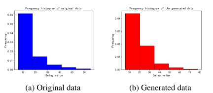
Fig. 2. Comparison of frequency distribution between generated and original data for terminal delays.
5. Train Delay Prediction Based on Data Fusion with Generated Data
The train operation data exhibit a strong spatiotemporal correlation. To enhance the ability of the model to capture temporal and spatial features, a CBLA neural network model was constructed for training delay prediction. Specifically, a CNN is first employed to extract multidimensional features from the training operation data. Subsequently, a bidirectional long short-term memory (BiLSTM) network was used to capture temporal dependencies in the data. Finally, an attention mechanism is introduced to enhance the focus of the model on delay-related key information. Detailed parameter settings for each network layer are listed in Table 7.
| Parameter name | Value |
| Number of CNN layers | 1 |
| CNN kernel size | 3 |
| Number of CNN kernels | 64 |
| Bi-LSTM hidden dimension | 64 |
| Number of Bi-LSTM layers | 2 |
| Time steps | 2 |
| Activation function | ReLU |
The specific procedure for training delay prediction based on the data generated by the improved CTGAN is as follows: First, raw train operation data were collected, and delay increments and scenario features were constructed based on train operation knowledge. Next, an improved CTGAN model was designed according to the constructed delay-related features and trained to learn the data distribution. Then, the trained improved CTGAN model was used to generate the training delay data. Subsequently, similarity-based evaluation metrics were used to assess the quality of the generated data. Finally, the generated data are combined with the original data to form an augmented dataset, which is used to train the delay prediction model. The trained model was then tested on the same dataset, and the prediction performances of the models trained on the original and augmented datasets were compared.
A network model was constructed based on the parameters listed in Table 7. The dataset was partitioned into training and validation sets that accounted for 85% and 15% of the total data, respectively. Model training was conducted using the training parameters listed in Table 8.
| Parameter | Value |
| Optimizer | Adam |
| Epochs | 1500 |
| Dropout rate | 0.1 |
| Input dimension | 2 |
| Number of input features | 4 |
| Batch size | 256 |
| Loss function | MAE |
A total of 1,725 delay records were collected from a specific railway line in China between 2019 and 2020. The synthetic delay data were generated at ratios of \({1{\times}}\), \({2{\times}}\), \({4{\times}}\), \({6{\times}}\), and \({8{\times}}\) relative to the original dataset. Considering that the proportion of generated data to real data may affect the model performance, different amounts of data were randomly generated such that the ratios of generated data to original data were \({8:1}\), \({6:1}\), \({4:1}\), \({2:1}\), and \({1:1}\).
The augmented datasets obtained by fusing data with different ratios as well as the original dataset were used as the training sets for the CBLA prediction model. Based on the test outputs of the trained model, error metrics including the mean absolute error (MAE) and root mean square error (RMSE) were calculated. The results are presented in Tables 9 and 10.
| Data type | Delay range [min] | |||
| \({<}10\) | \([10,30)\) | \({\geq}30\) | Overall | |
| Original | 0.218 | 0.947 | 5.305 | 0.513 |
| \({\text{Gen}: \text{Ori}}={8:1}\) | 0.302 | 0.620 | 1.318 | 0.381 |
| \({\text{Gen}: \text{Ori}}={6:1}\) | 0.335 | 0.683 | 1.496 | 0.427 |
| \({\text{Gen}: \text{Ori}}={4:1}\) | 0.247 | 0.699 | 0.830 | 0.316 |
| \({\text{Gen}: \text{Ori}}={2:1}\) | 0.230 | 0.905 | 2.159 | 0.386 |
| \({\text{Gen}: \text{Ori}}={1:1}\) | 0.229 | 0.827 | 1.942 | 0.370 |
| Data type | Delay range [min] | |||
| \({<}10\) | \([10,30)\) | \({\geq}30\) | Overall | |
| Original | 0.475 | 1.247 | 9.037 | 2.727 |
| \({\text{Gen}: \text{Ori}}={8:1}\) | 0.538 | 0.889 | 1.573 | 0.664 |
| \({\text{Gen}: \text{Ori}}={6:1}\) | 0.569 | 0.877 | 1.700 | 0.704 |
| \({\text{Gen}: \text{Ori}}={4:1}\) | 0.472 | 1.028 | 1.114 | 0.591 |
| \({\text{Gen}: \text{Ori}}={2:1}\) | 0.464 | 1.116 | 3.509 | 0.924 |
| \({\text{Gen}: \text{Ori}}={1:1}\) | 0.462 | 1.044 | 2.494 | 0.766 |
In Tables 9 and 10, “\({\text{Gen}: \text{Ori}}\)” denotes the ratio of CTGAN-generated data to the original data. According to the results shown in Tables 9 and 10, the delay prediction model trained on the dataset constructed by fusing the data generated by the improved CTGAN with the original data achieved the best overall performance, with an MAE of 0.316 min and an RMSE of 0.591 min. By contrast, when the model was trained using only the original dataset, the overall MAE and RMSE were 0.513 and 2.727 min, respectively. Comparatively, the use of fused data reduced the MAE by approximately 38% and the RMSE by approximately 78%, indicating a significant improvement in prediction performance.
Furthermore, a detailed analysis was conducted under different delay scenarios by categorizing the delay samples into three intervals: less than 10, 10–30, and greater than 30 min. For small delays (less than 10 min), the prediction errors of the models trained on the original and fused datasets were comparable. However, as the delay duration increased, the performance gap between the two models became more pronounced. In particular, for large delays (greater than 30 min), the best prediction results obtained using the fused dataset yielded an MAE of 0.830 min and an RMSE of 1.114 min, which were reduced by approximately 80% and 87%, respectively, compared with those obtained using the original dataset. These results demonstrate that the fused data significantly improve the prediction performance in large-delay scenarios where samples are relatively scarce.
Table 9 also shows that the delay prediction performance reached its optimum when the ratio of generated to original data was \({4:1}\), whereas fusion ratios that were either too low or too high adversely affected the results. When the proportion of generated data was excessively high, the predictive performance for small-delay samples (0–10 min) decreased. For instance, at ratios of \({8:1}\) or \({6:1}\), the MAE for 0–10 min samples exceeds 0.3 min, compared to 0.218 min for the original data. Combined with the scatter plot (Fig. 3), it can be observed that an excessive proportion tends to lead to an overestimation of small delay samples, which causes the total number of large delay samples to increase disproportionately, thereby obscuring the underlying patterns of small delays within the real data. Conversely, when the proportion was too small (e.g., \({2:1}\) or \({1:1}\)), the performance for large-delay samples (\({>}30\) min) deteriorated with an MAE of approximately 2 min. However, when the ratio exceeds \({2:1}\), the MAE for samples exceeding 30 min decreases to approximately 1.4 min.
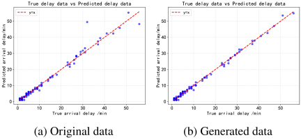
Fig. 3. Comparison of delay prediction performance between original data and CTGAN-augmented data.
To illustrate the delay prediction performance of the models trained on different datasets more intuitively, scatter plots of all test samples were constructed, where the horizontal axis represents the actual arrival delay and the vertical axis represents the predicted arrival delay. The results are shown in Fig. 3(a), which presents the prediction results obtained from the model trained on the original dataset, while Fig. 3(b) shows the prediction results obtained from the model trained on the dataset formed by fusing the generated data with the original data at a ratio of \({4:1}\).
The red diagonal line in Fig. 3 represents the conditions under which the predicted values are equal to the true values. The closer the scatter points were to the diagonal line, the closer the predictions were to the ground truth. Fig. 3 shows that for delays greater than 30 min, the prediction results based on the original dataset show significant deviations from the true values. In contrast, when the CTGAN-generated data were fused with the original data, the scatter points were more closely aligned with the diagonal line, indicating better agreement with the true values. In particular, the prediction performance for large-delay scenarios (greater than 30 min) improved significantly. This demonstrates that the data generated by the improved CTGAN model can effectively alleviate the issue of insufficient samples in large-delay scenarios, thereby enhancing the accuracy of delay forecasting.
6. Conclusion
This study performed CBLA high-speed railway train delay prediction based on the generated data fusion. By designing an improved CTGAN model, the feature correlations of delay scenarios within the original data were captured to generate synthetic delay samples. These generated samples are fused with real data to construct an augmented train delay dataset, effectively addressing the sparsity of the major delay samples in the original data. The augmented dataset was used to train the CBLA delay-prediction model. The experimental results determined the optimal data fusion ratio and demonstrated that data fusion using the improved CTGAN-generated data significantly enhanced the prediction accuracy of the CBLA model, particularly in scenarios where the data were limited and major delay samples were sparse. The prediction performance reached its optimum when the ratio of the generated to the original data was \({4:1}\), with the MAE reduced by approximately 38% and the RMSE reduced by approximately 78%.
Acknowledgments
This work was supported in part by the National Natural Science Foundation of China under Grant 62203468, Technological Research and Development Program of China State Railway Group Co., Ltd. under Grant N2024G040, Research Program of China Academy of Railway Sciences Co., Ltd. under Grant 2025YJ327, and Research Program of the Signal and Communication Research Institute under Grant 2025HT03.
- [1] X. Zhou et al., “Research on multiple rules flexible configuration method for default arrival and departure tracks in intelligent CTC system,” Railw. Signal. Commun., Vol.61, No.10, pp. 9-15, 2025 (in Chinese). https://doi.org/10.13879/j.issn.1000-7458.2025-10.25002
- [2] L. Liu et al., “Research on intelligent operation and maintenance system of centralized traffic control system based on edge-cloud collaboration,” Railw. Signal. Commun., Vol.62, No.3, pp. 8-14, 2026 (in Chinese). https://doi.org/10.13879/j.issn.1000-7458.2026-03.25308
- [3] J. Wang, “Study on intelligent centralized traffic control system,” Railw. Signal. Commun., Vol.58, No.7, pp. 7-12, 2022 (in Chinese). https://doi.org/10.13879/j.issn.1000-7458.2022-07.21395
- [4] Z. Fu, Z. Wang, Y. Song, and W. Xu, “Research on optimization scheme of station information acquisition technology for TDCS/CTC systems,” Railw. Signal. Commun., Vol.61, No.11, pp. 26-33, 2025 (in Chinese). https://doi.org/10.13879/j.issn.1000-7458.2025-11.25052
- [5] S. Ding, T. Zhang, R. Wang, and Z. Yuan, “Research on rescheduling of arrival and departure tracks at high-speed railway passenger station,” Railw. Signal. Commun., Vol.58, No.8, pp. 32-36, 2022 (in Chinese). https://doi.org/10.13879/j.issn.1000-7458.2022-08.21484
- [6] M. M. Dessouky and R. C. Leachman, “A simulation modeling methodology for analyzing large complex rail networks,” Simulation, Vol.65, No.2, pp. 131-142, 1995. https://doi.org/10.1177/003754979506500205
- [7] Q. Lu, M. Dessouky, and R. C. Leachman, “Modeling train movements through complex rail networks,” ACM Trans. Model. Comput. Simul., Vol.14, No.1, pp. 48-75, 2004. https://doi.org/10.1145/974734.974737
- [8] A. Moeinaddini, Y. Shafahi, and R. M. Hasany, “A simulation model for train movements in the rail network,” Proc. Inst. Civ. Eng. Transp., Vol.172, No.3, pp. 152-163, 2019. https://doi.org/10.1680/jtran.16.00082
- [9] E. R. Petersen and A. J. Taylor, “A structured model for rail line simulation and optimization,” Transp. Sci., Vol.16, No.2, pp. 192-206, 1982. https://doi.org/10.1287/trsc.16.2.192
- [10] S. F. Hallowell and P. T. Harker, “Predicting on-time performance in scheduled railroad operations: Methodology and application to train scheduling,” Transp. Res. A: Policy Pract., Vol.32, No.4, pp. 279-295, 1998. https://doi.org/10.1016/S0965-8564(97)00009-8
- [11] P. Murali, M. Dessouky, F. Ordóñez, and K. Palmer, “A delay estimation technique for single and double-track railroads,” Transp. Res. E: Logist. Transp. Rev., Vol.46, No.4, pp. 483-495, 2010. https://doi.org/10.1016/j.tre.2009.04.016
- [12] M. del Álamo, J. Heusel, and D. Narezo Guzmán, “Synthetic data generation for condition monitoring of railway switches,” Dependable Computing – EDCC 2022 Workshops, pp. 76-88, 2022. https://doi.org/10.1007/978-3-031-16245-9_6
- [13] S. Qiu et al., “Automated detection of railway defective fasteners based on YOLOv8-FAM and synthetic data using style transfer,” Autom. Constr., Vol.162, Article No.105363, 2024. https://doi.org/10.1016/j.autcon.2024.105363
- [14] G. D’Amico et al., “TrainSim: A railway simulation framework for LiDAR and camera dataset generation,” IEEE Trans. Intell. Transp. Syst., Vol.24, No.12, pp. 15006-15017, 2023. https://doi.org/10.1109/TITS.2023.3297728
- [15] G. Salierno, L. Leonardi, and G. Cabri, “A big data architecture for digital twin creation of railway signals based on synthetic data,” IEEE Open J. Intell. Transp. Syst., Vol.5, pp. 342-359, 2024. https://doi.org/10.1109/OJITS.2024.3412820
- [16] B. Yan et al., “Semantic segmentation of railway infrastructure based on virtual model synthetic data,” IEEE 26th Int. Conf. Intell. Transp. Syst. (ITSC), pp. 3831-3836, 2023. https://doi.org/10.1109/ITSC57777.2023.10422077
- [17] I. Goodfellow et al., “Generative adversarial networks,” Commun. ACM, Vol.63, No.11, pp. 139-144, 2020. https://doi.org/10.1145/3422622
- [18] L. Xu and K. Veeramachaneni, “Synthesizing tabular data using generative adversarial networks,” arXiv:1811.11264, 2018. https://doi.org/10.48550/arXiv.1811.11264
- [19] L. Xu, M. Skoularidou, A. Cuesta-Infante, and K. Veeramachaneni, “Modeling tabular data using conditional GAN,” Adv. Neural Inf. Process. Syst., Vol.32, pp. 7335-7345, 2019.
- [20] N. L. Agu, S. M. Haider, G. G. Pillai, I. Bashir, and G. Lacey, “Power transformer DGA data augmentation using conditional tabular generative adversarial network,” 59th Int. Univ. Power Eng. Conf. (UPEC), 2024. https://doi.org/10.1109/UPEC61344.2024.10892386
- [21] A. Alzahrani, “Early detection of lung cancer using predictive modeling incorporating CTGAN features and tree-based learning,” IEEE Access, Vol.13, pp. 34321-34333, 2025. https://doi.org/10.1109/ACCESS.2025.3543215
- [22] W. Li et al., “EID-GAN: Generative adversarial nets for extremely imbalanced data augmentation,” IEEE Trans. Ind. Inform., Vol.19, No.3, pp. 3208-3218, 2023. https://doi.org/10.1109/TII.2022.3182781
- [23] R. Liu et al., “Anomaly-GAN: A data augmentation method for train surface anomaly detection,” Expert Syst. Appl., Vol.228, Article No.120284, 2023. https://doi.org/10.1016/j.eswa.2023.120284
This article is published under a Creative Commons Attribution-NoDerivatives 4.0 Internationa License.