Research Paper:
Tsallis Entropy-Regularized Fuzzy c-Varieties
Haruki Kobayashi and Yuchi Kanzawa

Shibaura Institute of Technology
3-7-5 Toyosu, Koto-ku, Tokyo 135-8548, Japan

Fuzzy c-means (FCM) and its variants, including entropy-regularized FCM and Tsallis entropy-based FCM (TFCM), are widely used in fuzzy clustering. Although these algorithms are effective, they cannot model the cluster-specific subspaces that are often present in high-dimensional data. To address this limitation, fuzzy c-varieties (FCV) represent each cluster as a low-dimensional variety and iteratively alternate between dimension reduction and clustering, thereby capturing intrinsic cluster structures. Building on this, we propose a Tsallis entropy-regularized FCV (TFCV), which generalizes both standard FCV (SFCV) and entropy-regularized FCV (EFCV) by regularizing the SFCV objective with Tsallis entropy. TFCV inherits the enhanced flexibility of TFCM, leading to improved clustering performance. Theoretical analysis of the fuzzy classification functions confirmed that TFCV generalizes SFCV and EFCV. Empirical evaluations on 14 real datasets demonstrated that TFCV achieves a higher clustering accuracy than the existing methods with statistical significance, establishing its effectiveness as a robust approach that integrates dimension reduction and fuzzy clustering.
FCF example of TFCV
1. Introduction
Fuzzy \(c\)-means (FCM) 1 is widely recognized as a prototypical algorithm for fuzzy clustering. To distinguish it from its extensions, it is commonly referred to as the standard FCM (SFCM). Several variants have been proposed, including entropy-regularized FCM (EFCM) 2 and Tsallis entropy-based FCM (TFCM) 3. TFCM is formulated by incorporating Tsallis entropy regularization into SFCM 4, thereby serving as a generalization of both SFCM and EFCM. By adjusting its fuzzification parameters, TFCM yields more flexible clustering structures and frequently achieves improved accuracy compared to SFCM and EFCM.
Individuals often lie in subspaces with a lower dimensionality than the apparent ambient space, and capturing such subspaces is crucial for understanding the intrinsic structure of data. However, FCM and its variants lack a mechanism for modeling these underlying subspaces. A seemingly straightforward solution is to apply a dimension-reduction method, such as principal component analysis (PCA), before clustering. This approach may appear attractive, as it enables more efficient application of the FCM family in a reduced-dimensional space than in the original but unnecessarily high-dimensional space. Nevertheless, applying PCA globally to an entire dataset risks overlooking clusters associated with distinct subspaces. For example, consider two clusters embedded in a 2D space, each generated from a 1D subspace orthogonal to the other. Any global reduction of objects to a single 1D space inevitably obscures one or both the cluster-specific subspaces. To address this limitation, the fuzzy \(c\)-varieties (FCV) 5 algorithm was proposed. This algorithm represents each cluster by a low-dimensional variety and alternates between two procedures: identifying the variety through a dimensionality-reduction step akin to PCA, and clustering objects based on their dissimilarity to the variety associated with each cluster. Through this iterative procedure, the FCV successfully captures cluster-specific subspaces, thereby providing a more faithful representation of the data structure.
Given that FCV employs the same fuzzification method as SFCM, we refer to it as the standard FCV. Moreover, analogous to SFCV, which simultaneously performs dimension reduction and clustering, another variant has been proposed that incorporates Shannon entropy regularization such as EFCM, which we refer to as entropy-regularized FCV (EFCV) 6. Because TFCM—a generalization of both SFCM and EFCM—has demonstrated superior clustering performance through its enhanced flexibility, it is reasonable to expect that an algorithm generalizing both SFCV and EFCV would achieve even higher clustering accuracy in approaches that integrate dimension reduction and clustering. This consideration served as a key impetus for developing the proposed algorithm.
In this paper, we propose Tsallis entropy-regularized fuzzy \(c\)-varieties (TFCV). This algorithm is derived from an optimization problem in which the SFCV objective function is regularized using Tsallis entropy. Thus, TFCV directly generalizes SFCV and has also been shown to generalize EFCV in terms of objective functions. Furthermore, we demonstrated that TFCV generalizes both SFCV and EFCV with respect to their update rules. In numerical experiments using an artificial dataset, the intrinsic properties of SFCV, EFCV, and TFCV were clarified by observing their corresponding fuzzy classification functions (FCFs) 7. Notably, revealing the relationships between the algorithms through the observation of FCFs represents the first such attempt for both the proposed algorithm, TFCV, and the conventional algorithms, SFCV and EFCV. These experiments corroborated the theoretical finding that TFCV generalizes both SFCV and EFCV. Furthermore, we demonstrated that at the intersection of varieties corresponding to cluster representatives, the FCF of SFCV is undefined. In contrast, the FCF of EFCV is well defined and equals the reciprocal of the number of clusters. Notably, TFCV, which generalizes both SFCV and EFCV, inherits the property of EFCV and equals the reciprocal of the number of clusters. In addition, experiments using 14 real datasets showed that the proposed TFCV achieved a significantly higher clustering accuracy than the conventional SFCV and EFCV algorithms.
The remainder of this paper is organized as follows. In Section 2, we introduce the notations and the existing conventional algorithms. Section 3 describes our proposed clustering algorithm. Section 4 presents the results of numerical experiments conducted to validate the effectiveness of the proposed algorithm. Finally, we conclude the paper in Section 5.
2. Preliminaries
2.1. Shannon Entropy and Tsallis Entropy
Let \(P\) be the probability distribution. The Shannon entropy of \(P\), denoted \(H_{\text{Shannon}}(P)\), is defined as follows.
2.2. Conventional Fuzzy Clustering Algorithms
2.2.1. Family of Fuzzy \(c\)-Means Algorithms
We consider the task of partitioning a dataset of \(D\)-dimensional observations, \(X=\{x_k \mid{} x_k\in\mathbb{R}^D, k\in\{1,\dots,N\}\}\), into \(C\) clusters. The fuzzy membership is denoted as \(u=\{ u_{i,k} \mid{} u_{i,k}\in [0,1], i\in\mathbb\{1,\dots,C\},k\in\mathbb\{1,\dots,N\}\}\), where \(u_{i,k}\) represents the degree of belongingness between object \(x_k\) and the \(i\)-th cluster. These membership values must satisfy the following normalization constraint:
2.2.2. Family of Fuzzy \(c\)-Varieties Algorithms
Let \(w=\{ w_{i,d'} \mid{} w_{i,d'}\in\mathbb{R}^D, i\in\mathbb\{1,\dots,C\},d'\in\mathbb\{1,\dots,D'\}\}\) denote the set of basis vectors spanning the subspace of the \(i\)-th cluster, where \(D'\) denotes the dimension of the subspace. \(w\) satisfies the following constraint:
Algorithm 1—SFCV and EFCV:
- Step 1.
Specify the cluster number \(C\), the dimension of subspace \(D'\). Set the fuzzification parameters \(m>1\) for SFCV, and \(\lambda>0\) for EFCV. Initialize the membership \(u\).
- Step 2.
Calculate the initial cluster center \(v\) using
\begin{align} & v_i=\dfrac{ \displaystyle\sum_{k=1}^N \left(u_{i,k}\right)^m x_k }{ \displaystyle\sum_{k=1}^N \left(u_{i,k}\right)^m }\quad(i\in\{1,\dots,C\}), \label{eq:v-SFCV} \end{align}for SFCV, and
\begin{align} & v_i=\dfrac{ \displaystyle \sum_{k=1}^Nu_{i,k} x_k }{ \displaystyle \sum_{k=1}^Nu_{i,k} } \quad (i\in\{1,\dots,C\}).\label{eq:v-EFCV} \end{align}for EFCV.
- Step 3.
Obtain \(w\) by constructing from the eigenvectors associated with the \(D'\) space’s largest eigenvalues of the matrix \(\sum_{k=1}^N(u_{i,k})^m(x_k-v_i)(x_k-v_i)^\mathsf{T}\) for SFCV, and \(\sum_{k=1}^Nu_{i,k}(x_k-v_i)(x_k-v_i)^\mathsf{T}\) for EFCV sorted in descending order.
- Step 4.
Evaluate the dissimilarity between the objects and the cluster centers \(d\) using Eq. \(\eqref{eq:d-FCV}\).
- Step 5.
Update the membership \(u\) using
\begin{align} u_{i,k}&=\left[ \sum_{j=1}^C \left(\frac{d_{i,k}}{d_{j,k}} \right)^{\frac{1}{m-1}} \right]^{-1} \quad(i\in\{1,\dots,C\}) ,\label{eq:u-SFCV} \end{align}for SFCV, and
\begin{align} u_{i,k}=\left[ \sum_{j=1}^C \exp\left(\lambda \left(d_{i,k}-d_{j,k}\right)\right) \right]^{-1} ~~(i\in\{1,\dots,C\}) , \label{eq:u-EFCV} \end{align}for EFCV.
- Step 6.
Assess the convergence of \((u, v, w)\). If the stopping criterion is not met, return to Step 2.
∎
An FCF characterizes the extent to which a point in an object space belongs to each cluster by distributing the membership values over the entire space. This function provides a convenient means for highlighting the characteristics of fuzzy clustering algorithms. The FCFs for SFCV and EFCV, denoted by \(u(x)=\{u_i(x) \in [0,1],i\in\{1,\dots,C\}\}\) corresponding to a new point \(x \in \mathbb{R}^D\), are defined as
3. Proposed Algorithm
We propose a new algorithm called Tsallis entropy-regularized fuzzy \(c\)-varieties (TFCV). Given that the application of Tsallis entropy regularization to SFCM has been shown to yield higher clustering accuracy than both SFCM and EFCM, we designed an extended optimization framework. Specifically, the objective function of the SFCV in Eq. \(\eqref{eq:SFCV-objective}\) was modified by incorporating a Tsallis entropy regularization term, leading to the following TFCV optimization problem:
The TFCV algorithm is derived as follows. First, we define the Lagrangian function as
Algorithm 2—TFCV:
- Step 1.
Specify the number of clusters \(C\) and the dimension of subspace \(D'\). Set the fuzzification parameters \(m>1\) and \(\lambda>0\). Initialize membership \(u\).
- Step 2.
Calculate the initial cluster center \(v\) using Eq. \(\eqref{eq:v-TFCV}\).
- Step 3.
Obtain \(w\) by constructing from the eigenvectors associated with the \(D'\) space largest eigenvalues of matrix \(\sum_{k=1}^N (u_{i,k})^{m}(x_k-v_i)(x_k-v_i)^\mathsf{T}\), sorted in descending order.
- Step 4.
Evaluate the dissimilarities \(d\) between the objects and cluster centers using Eq. \(\eqref{eq:d-FCV}\).
- Step 5.
Update membership \(u\) using Eq. \(\eqref{eq:u-TFCV}\).
- Step 6.
Assess the convergence of \((u, v, w)\). If the stopping criterion is not met, return to Step 2.
∎
Note that numerical overflow or “not a number” (NaN) values may occur in computation when using extreme values of \(m\) or \(\lambda\), as follows. When the parameter \(m\) is set extremely close to 1—for example, \(m=1+10^{-16}\)—floating-point rounding may cause \(1-m\) to be evaluated as zero. In such cases, the exponent appearing in the membership update given in Eq. \(\eqref{eq:u-TFCV}\) become NaN, and the iteration cannot proceed. This issue also arises in conventional SFCM algorithms. Conversely, if \(m\) is selected to be extremely large, such as \(m=10^{300}\), the terms of the form \((1-(1-m)\lambda d_{i,k})\) in the membership update formula may overflow. In the update of the cluster centers \(v\) given in Eq. \(\eqref{eq:v-TFCV}\), the denominator may underflow to zero, which can lead to NaN values and terminate the computation. This issue also arises in conventional SFCM algorithms. If the parameter \(\lambda\) is set to an extremely large (e.g., \(\lambda=10^{300}\)), the same overflow problem can occur in the membership update step for the terms \((1-(1-m)\lambda d_{i,k})\).
At the beginning of this section, TFCV was noted as a generalization of both SFCV and EFCV using their objective functions. We observe that TFCV generalizes both SFCV and EFCV at the algorithm level.
First, we observe that TFCV is a generalization of the SFCV. The first four steps of TFCV (Algorithm 2) are identical to those of SFCV (Algorithm 1). Although Step 5 in TFCV seems to differ from that in SFCV, the TFCV membership equation in Eq. \(\eqref{eq:u-TFCV}\) can be reduced to the SFCV membership equation (Eq. \(\eqref{eq:u-SFCV}\)) in the limit \(\lambda\to\infty\), as follows:
Next, we observe that TFCV is also a generalization of EFCV. Step 1 of TFCV coincides with that of EFCV, and Steps 2 and 3 reduce to their EFCV counterparts when \(m=1\). Step 4 is identical for both methods. Although Step 5 in the TFCV differs in form, the membership equation in Eq. \(\eqref{eq:u-TFCV}\) converges to the EFCV membership equation expressed in Eq. \(\eqref{eq:u-EFCV}\) as \(m\searrow1\):
The above discussions and those at the beginning of this section show that TFCV generalizes both SFCV and EFCV at both the objective function and algorithm levels.
The FCF of TFCV, denoted by \(u(x)=\{u_i(x) \in \mathbb{R},i\in\{1,\dots,C\}\}\) regarding new object \(x\in\mathbb{R}^D\), is defined as
4. Numerical Experiments
4.1. Behaviors of FCFs for SFCV, EFCV, and TFCV
In the first experiment, we analyzed the behaviors of the FCFs for SFCV, EFCV, and TFCV. Furthermore, we observed a close relationship between TFCV and existing conventional algorithms. In this experiment, we applied TFCV, SFCV, and EFCV to an artificial dataset, as illustrated in Fig. 1, which formed two linear clusters in a 2D space. Notably, across all variations in the fuzzification parameter values, the proposed algorithm consistently yielded satisfactory clustering results, as shown in Fig. 2 (objects belonging to Cluster #1 are shown in green and those in Cluster #2 are shown in red), with \(v_1 \simeq v_2 \simeq (0, 0)^\mathsf{T}\), \(w_{1,1} \simeq (0, 1)^\mathsf{T}\), and \(w_{2,1} \simeq (1, 0)^\mathsf{T}\). Note that the cluster center \(v_1\), indicated by a green cross, is not visible in the figure because it coincides with \(v_2\), and the red cross marker for \(v_2\) completely overlays it.
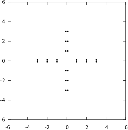
Fig. 1. Artificial dataset.
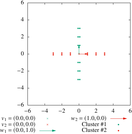
Fig. 2. Visualization of proper clustering result.
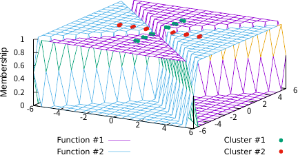
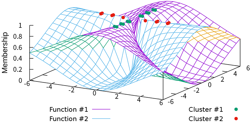
Fig. 3. TFCV (\((m, \lambda)=(1.01, 100)\)).
To avoid misunderstanding, we emphasize that the purpose of this experiment was not to evaluate the clustering performance of the methods. Artificially simple dataset was deliberately selected so that the differences in algorithmic behavior with respect to the tuning parameters could be clearly observed, without the confounding effects of complex data structures. A thorough performance comparison between the proposed method and conventional methods on multiple real datasets is presented in the next subsection.
Figures 3–5 illustrate the FCFs of TFCV with various fuzzification parameter values. For comparison, Fig. 6 shows the FCF of SFCV with \(m=2\) and Fig. 7 shows the FCF of EFCV with \(\lambda=0.2\). In these figures, objects belonging to the first cluster are shown as green points, those in the second cluster as red points, and the FCFs for the first and second clusters are represented by purple and sky-blue surfaces, respectively. The base plane represents the data space and the vertical axis indicates the FCF value. Figs. 3 and 4 show the effect of the fuzzification parameter \(m\) on the FCF and the clustering results, indicating that larger values of \(m\) produce a fuzzier clustering in regions away from all objects. Figs. 3 and 5 indicate the effect of parameter \(\lambda\); smaller values of \(\lambda\) produce fuzzier clustering in regions where \(u_1(x)=u_2(x)\). Note that Figs. 4 and 6 are similar, which substantiates the theoretical result that TFCV with \(\lambda\to\infty\) is reduced to SFCV shown in the previous section. In addition, Figs. 5 and 7 are similar, which substantiates the theoretical result that TFCV with \(m\searrow1\) was reduced to EFCV, as shown in the previous section.
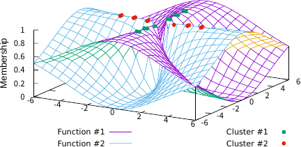
Fig. 4. TFCV (\((m, \lambda)=(2, 100)\)).
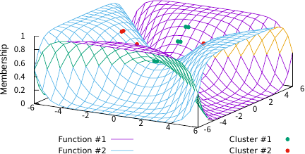
Fig. 5. TFCV (\((m, \lambda)=(1.01, 0.2)\)).

Fig. 6. SFCV (\(m=2\)).
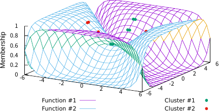
Fig. 7. EFCV (\(\lambda=0.2\)).
In Fig. 6, the FCF values \(u_1(x)\) on the subspace \(v_1+\alpha w_{1,1}\) (\(\alpha \in \mathbb{R}\)) seems to be similar to that of \(u_2(x)\) on the subspace \(v_2+\alpha w_{2,1}\) (\(\alpha \in \mathbb{R}\)). This raises to the question of the FCF value at \(x= (0, 0)^\mathsf{T}\), the intersection point of the two subspaces because the FCF constraint \(u_1(x)+u_2(x)=1\) implies that \(u_1(0)=1\) and \(u_2(0)=1\) cannot hold simultaneously. We address this question theoretically, and show that the FCF value of SFCV at \(x= (0, 0)^\mathsf{T}\) is not well-defined as it depends on the direction from which \(x\) approaches this point. First, we consider limit \(a\to0\) with \(x=(a, 0)\), where \(a\in\mathbb{R}\setminus {0}\). In this setting, the values of \(d_1(x)\) and \(d_2(x)\) are calculated using Eq. \(\eqref{eq:d-FCV-FCF}\), as follows:
TFCV generalizes both SFCV and EFCV from the perspectives of both the optimization problem and the algorithm. This fact, along with the above discussion, yields another question: whether the FCF value of TFCV is well-defined at \(x= (0, 0)^\mathsf{T}\). We show that the FCF value of TFCV at \(x= (0, 0)^\mathsf{T}\) is well-defined, inheriting the property of EFCV because we have
4.2. Comparison of Clustering Accuracy Using Real Datasets
In the second set of experiments, we assessed the clustering performance of the proposed algorithm in comparison with conventional approaches across 14 real datasets. The Breast Cancer Coimbra (BCC), Breast Cancer Wisconsin (Original) (BCW), Glass Identification (Glass), Optical Recognition of Handwritten Digits (Optdigits), Seeds, and Yeast datasets were obtained from the UCI Machine Learning repository 8. The Coffee and Olive datasets were retrieved from the pgmm package 9 in R, whereas the Crabs dataset was retrieved from the MASS package 10 in R. The Wine dataset was accessed using the rattle package 11, and the Australian Institute of Sport (AIS) dataset was obtained from the Australasian Data and Story Library 12. Bupa and Heart data were obtained from the Keel website at University of Granada 13, and Pima Indians Diabetes (PID) data were obtained from the Kaggle website 14.
All datasets were clustered using SFCV, EFCV, and the proposed TFCV algorithms. For each dataset, the number of clusters was fixed to match the number of ground truth classes. Table 1 summarizes the characteristics of the datasets, including the number of objects, clusters, and dimensions.
Table 1. Real datasets.

The fuzzification parameters were varied according to the following rationale. As observed in the artificial data experiments, a larger value of \(m\) yielded fuzzier clustering results, whereas a smaller value produced crisper clustering results. If \(m\) becomes excessively large, the membership degrees approach \(1/C\) for all objects, causing all cluster centers to collapse to a single point and resulting in a meaningless clustering structure. Conversely, if \(m\) is set too small, the memberships become overly crisp, forcing objects near cluster boundaries, where fuzzy assignments are inherently appropriate, to be assigned values close to \(1\) or \(0\), thereby degrading the clustering accuracy. Moreover, excessively small values of \(m\) can lead to numerical instability, eventually producing NaN values that prevent the algorithm from continuing. Similarly, a smaller value of \(\lambda\) yields fuzzier results, whereas a larger value produces crisper results. When \(\lambda\) is too small, the memberships again approach \(1/C\), causing all cluster centers to collapse and producing an uninformative clustering. On the other hand, if \(\lambda\) is set too large, the memberships become overly crisp, leading to the same degradation in accuracy near cluster boundaries. Furthermore, extremely large values of \(\lambda\) may cause numerical overflow, preventing the algorithm from proceeding. A clustering result that is excessively fuzzy and thus meaningless can be detected by the partition entropy (PE) 1; if the PE value associated with a result is equal to the logarithm of the number of clusters, the result is discarded because such a solution does not correspond to a meaningful clustering structure. Considering this, preliminary experiments were performed to identify the parameter ranges that avoid overflow or NaN values, yielding a PE value lower than \(\ln(C)\). Balancing these considerations, we varied the parameter values as follows: \(m \in \{1+10^{-15}\), \(1+10^{-10}\), \(1+10^{-5}\), \(1+10^{-3}\), \(1+10^{-2}\), \(1.1\), \(1.5\), \(2.0\), \(3.0\), \(4.0\), \(5.0\), \(10.0\}\) and \(\lambda \in \{0.001\), \(0.01\), \(0.1\), \(0.5\), \(1.0\), \(1.5\), \(2.0\), \(5.0\), \(10\), \(100\), \(10^{3}\), \(10^{10}\}\). The dimensions of the subspace also influence clustering accuracy. In accordance with the general principle of dimensionality reduction that the data are expected to lie in relatively low-dimensional subspaces, we varied the dimension of subspace as follows: \(D'\in\{1, 2,\dots,\lceil D/2 \rceil\}\). For the Optdigits dataset, however, the dimension of subspace was varied as \(D'\in\{1, 2,\dots,10\}\) because of its higher intrinsic dimensionality. Each algorithm was executed ten times with randomly initialized memberships for every parameter setting, and the trial with the lowest objective function value was retained. Trials in which at least one object attained the highest membership value in two or more clusters were excluded from the analysis.
Table 2. ARI and PE values along with corresponding subspace dimensions and fuzzification parameter values.

Clustering quality was evaluated using the adjusted Rand index (ARI) 15, which is defined for unique crisp partitions. Consequently, trials where ties occurred at maximum membership values were excluded from the evaluation. Each algorithm also involves its own fuzzification parameter along with a certain dimension of the subspace as a hyperparameter. For each hyperparameter value, the highest ARI value was selected as the representative ARI for that algorithm on the given dataset.
Table 2 presents, for each dataset, the ARI values obtained by the three methods, SFCV, EFCV, and TFCV, along with the corresponding PE values and the parameter settings \((D', m, \lambda)\) under which these values were achieved. For each dataset, the five rows correspond to ARI, PE, \(D'\), \(m\), and \(\lambda\), respectively. Because SFCV does not use \(\lambda\) and EFCV does not use \(m\), the entries that do not apply are marked with “—.” The three columns represent SFCV, EFCV, and TFCV, respectively, and the highest ARI value for each dataset is highlighted in bold. Some readers may raise concerns that the clustering results for certain datasets are excessively fuzzy, based on the PE values reported in Table 2. In particular, for two-cluster datasets, PE values close to \(\ln(2)=0.6931\) may give the impression that the memberships are nearly uniform. However, a closer inspection of the detailed results shows that such values do not necessarily correspond to degenerating clustering solutions. For the BCW dataset, although the PE value of TFCV is relatively high (\(0.6888\)), the squared Euclidean distance between the two cluster centers is \(1.1063\), indicating that the centers do not form a single point. In addition, \(35\) out of the \(683\) objects have a membership difference of at least \(0.2\) (i.e., one membership is \(\ge 0.6\) and the other is \(\le 0.4\)), confirming that a meaningful clustering structure is preserved. The PE value of SFCV (\(0.6861\)) is slightly lower and likewise does not indicate a degenerate solution. A similar interpretation applies to the PID dataset. Although the PE value of SFCV is \(0.6383\), the squared distance between the two cluster centers is \(1421.6830\), and \(526\) out of the \(768\) objects exhibit a membership difference of at least \(0.2\). These observations indicate that the obtained clustering structure is nontrivial. The PE value of TFCV (\(0.6264\)) is lower yet and does not suggest excessive fuzziness. These observations confirm that the resulting clustering is not excessively fuzzy and retains interpretable structure. Readers may also raise the following concern: EFCV, which has only the fuzzification parameter \(\lambda\), does not seem to perform as well as SFCV, which has only the parameter \(m\). If this is the case, a question may arise whether the proposed method—TFCV, which incorporates both \(m\) and \(\lambda\)—can truly achieve better performance. This concern can be addressed as follows. The experiments using artificial datasets demonstrated that \(m\) and \(\lambda\) exhibit distinct and complementary effects on fuzzification behavior. Consequently, TFCV, which simultaneously utilizes both parameters, is capable of providing greater flexibility in controlling the degree of fuzziness and therefore has the potential to achieve higher clustering accuracy than methods that rely on only one of them. For the Yeast dataset, SFCV achieves an ARI of \(0.0849\) at \(m = 1.01\), and EFCV achieves the ARI of \(0.0779\) at \(\lambda = 1000.0\). In contrast, TFCV attains a higher ARI of \(0.0952\) when evaluated with the identical parameter values \(m = 1.01\) and \(\lambda = 1000.0\) that yielded the best results for SFCV and EFCV, respectively. For Optdigits dataset, SFCV achieves an ARI of \(0.6007\) at \(m = 1.1\). However, at the same parameter value \(m = 1.1\), TFCV achieves a higher ARI of \(0.6425\) under \(\lambda = 2.0\). These values illustrate the advantage of combining the two fuzzification parameters within a unified framework. Fig. 8 provides a boxplot visualization of the ARI values shown in Table 2. This figure is included to present the relative performance of the algorithms in an intuitive manner and to illustrate the overall tendency of their clustering accuracy across the 14 datasets. The median ARI achieved by TFCV was \(0.2432\), outperforming those of both SFCV (\(0.2217\)) and EFCV (\(0.2139\)). The Wilcoxon signed-rank test with Holm correction confirmed the statistical significance of these improvements (\(p=0.0359\) and \(p=0.0152\), respectively). These results demonstrate that TFCV provides a better performance advantage than SFCV and EFCV, because TFCV serves as a generalization for both algorithms.
Unfortunately, for datasets such as Seeds, Crabs, AIS, and Heart, performance improvement was not observed for any of the methods. However, the underlying mechanism remains unclear. In short, the power-based fuzzification controlled by \(m\) in SFCV and TFCV and the entropy-based fuzzification controlled by \(\lambda\) in EFCV and TFCV do not appear to provide differential advantages for enhancing clustering accuracy on these datasets. This suggests that achieving higher accuracy for such datasets may require a third type of fuzzification mechanism that is distinct from both the power-based and entropy-based approaches. Further, in the context of combining dimensionality reduction with fuzzy clustering, which is the central topic of this study, improving the accuracy is not limited to modifications of the fuzzification scheme. In this study, we restricted the dimensionality-reduction step to PCA and explored the effects of alternative fuzzification strategies under this framework. For these datasets, improved clustering performance may be obtained by adopting different dimensionality reduction techniques, such as probabilistic PCA. Investigating these approaches is an important direction for future research.
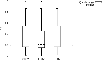
Fig. 8. Quartile range of ARI.
5. Conclusion
In this study, a new clustering algorithm called TFCV is proposed. Analysis of artificial data revealed the effects of fuzzification parameter \(m\) and regularization coefficient \(\lambda\) on the algorithm behavior, and elucidated its connection to traditional approaches. Subsequent experiments on 14 real datasets further showed that TFCV achieved superior clustering accuracy compared to alternative algorithms. In future work, we aim to extend this strategy to other dimension-reduction-based methods such as probabilistic PCA.
- [1] J. C. Bezdek, “Pattern Recognition with Fuzzy Objective Function Algorithms,” Plenum Press, 1981. https://doi.org/10.1007/978-1-4757-0450-1
- [2] S. Miyamoto and M. Mukaidono “Fuzzy c-Means as a Regularization and Maximum Entropy Approach,” Proc. 7th Int. Fuzzy Systems Association World Congress (IFSA’97), pp. 86-92, 1997.
- [3] M. Ménard, V. Courboulay, and P.-A. Dardignac, “Possibilistic and Probabilistic Fuzzy Clustering: Unification within the Framework of the Non-extensive Thermostatistics,” Pattern Recognition, Vol.36, No.6, pp. 1325-1342, 2003. https://doi.org/10.1016/S0031-3203(02)00049-3
- [4] C. Tsallis, “Possible Generalization of Boltzmann–Gibbs Statistics,” J. of Statistical Physics, Vol.52, Nos.1-2, pp. 479-487, 1988. https://doi.org/10.1007/BF01016429
- [5] J. C. Bezdek, C. Coray, R. Gunderson, and J. Watson, “Detection and Characterization of Cluster Substructure II. Fuzzy c c-Varieties and Convex Combinations Thereof,” SIAM J. on Applied Mathematics, Vol.40, No.2, pp. 358-372, 1981. https://doi.org/10.1137/0140030
- [6] G. E. Hinton, P. Dayan, and M. Revow, “Modeling the Manifolds of Images of Handwritten Digits,” IEEE Trans. on Neural Networks, Vol.8, No.1, pp. 65-74, 1997. https://doi.org/10.1109/72.554192
- [7] S. Miyamoto, H. Ichihashi, and K. Honda, “Algorithms for fuzzy clustering: Methods in c c-means clustering with applications,” Springer, 2008. https://doi.org/10.1007/978-3-540-78737-2
- [8] UCI Machine Learning Repository. https://archive.ics.uci.edu/ [Accessed August 11, 2025]
- [9] P. D. McNicholas, A. ElSherbiny, K. R. Jampani, A. F. McDaid, T. M. Murphy, and L. Banks, “pgmm: Parsimonious Gaussian Mixture Models,” R package, 2011. https://doi.org/10.32614/CRAN.package.pgmm
- [10] W. N. Venables and B. D. Ripley, “Modern Applied Statistics with S,” 4th ed., Springer, 2002. https://doi.org/10.1007/978-0-387-21706-2
- [11] G. Williams, “Data mining with Rattle and R: The art of excavating data for knowledge discovery,” Springer, 2011. https://doi.org/10.1007/978-1-4419-9890-3
- [12] G. K. Smyth, “Australasian Data and Story Library (OzDASL)," 2011. https://gksmyth.github.io/ozdasl [Accessed August 11, 2025]
- [13] Keel. http://www.keel.es. [Accessed December 23, 2025]
- [14] Kaggle, Pima Indians Diabetes Database. https://www.kaggle.com/datasets/uciml/pima-indians-diabetes-database [Accessed December 23, 2025]
- [15] L. Hubert and P. Arabie, “Comparing Partitions,” J. of Classification, Vol.2, No.1, pp. 193-218, 1985. https://doi.org/10.1007/BF01908075
This article is published under a Creative Commons Attribution-NoDerivatives 4.0 Internationa License.