Research Paper:
Total Fresh Weight Estimation Model for Herbaceous Plant Based on Improved YOLOv5 and 3D Point Clouds
Yitong Han
 and Xiangyang Xu†
Department of Automation, Beijing Institute of Technology
No.5 Zhongguancun South Street, Haidian District, Beijing 100081, China
†Corresponding author

The real-time quantitative estimation of herbaceous plant growth status holds significant potential for investigating fertilization effects, predicting growth curves, and enhancing crop yield. This study constructed a growth quantification model using an improved YOLOv5 architecture integrated with 3D point cloud processing, with pak choi as an exemplar crop. To improve the recognition accuracy while reducing the number of parameters, we employed a lightweight YOLOv5 model enhanced with Atrous Spatial Pyramid Pooling and Ghost convolution modules for individual pak choi plant localization and growth stage classification. We also developed a segmentation method based on the HSV color space to segment leaves. To estimate the total fresh weight of individual plants, we first calculated the leaf surface area by generating a triangular mesh from the corresponding leaf point clouds and predicted the chlorophyll content using a stacking ensemble model. Subsequently, to address the leaf occlusion issues, the leaf pixel ratio in the images, leaf surface area, and mean leaf chlorophyll content were collectively used as independent variables. Finally, a multiple linear regression model was developed to accurately estimate the total fresh weight of individual pak choi plants. Experimental results demonstrate that the modified YOLOv5 architecture achieves a 3.5% improvement in mAP@0.5 (reaching 96%) and a 4.66% increase in F1-score (attaining 90.26%), while significantly reducing the computational complexity compared to the baseline model. Statistical tests verified that the fitted equation could explain 79% of the variation in the total fresh weight, with an average relative error of 12.16%. This enables non-contact and accurate measurement of the pak choi growth status.
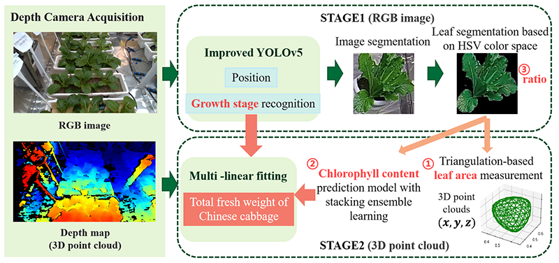
Pipeline of growth quantification
1. Introduction
Herbaceous plants, including rice, wheat, pak choi, and tobacco, exhibit extraordinary species diversity and wide distribution. These plants have significant agricultural and economic value. They are widely used in many fields such as food, medicine, spices, and cosmetics. Accurate real-time tracking of plant growth facilitates the study of the effects of fertilization and gene selection. It also lays the groundwork for predicting plant growth curves and enriches the research aimed at regulating herbaceous plant growth.
Currently, research on plant growth tracking falls into three main categories: manual detection, contact detection, and non-contact detection 1. Manual detection suffers from poor timeliness, low credibility, limited detection range, and a high cost of experience transfer, making it unsuitable for large-scale industrial production and cultivation. Lo Presti et al. 2 proposed equipping specific plant organs with wearable sensors based on fiber Bragg gratings (FBGs), which are expensive and susceptible to natural factors such as wind and rain in outdoor environments. Joshi et al. 3 proposed a wearable sensor for monitoring plant stomatal transpiration that is attached to the underside of leaves and may cause leaf lodging.
In recent years, the application of non-contact recognition based on image processing and remote sensing has become more widespread owing to its advantages of high efficiency, precision, real-time performance, and non-interference. Yulianto et al. 4 proposed the use of satellite imagery and radar-sensing technology to identify the growth stages of rice and predict its spatial distribution using the CART algorithm. This method is suitable for large-scale cultivation testing but cannot be used for detailed characterization. Song et al. 5 proposed the SEYOLOX-tiny model for detecting corn heading in the field, which achieved key feature extraction and noise suppression through an embedded attention mechanism, with an average accuracy of 95.0%, but lacked estimation of plant growth parameters. Zhu et al. 6 implemented direct triangular mesh reconstruction from wheat point clouds, enabling subsequent leaf semantic information extraction. This methodology represents a novel approach for monitoring plant growth.
Current research on plant growth status recognition is predominantly oriented towards qualitative classification, whereas quantitative estimation of biomass has received comparatively less attention. Furthermore, because of the unique morphological characteristics of herbaceous plants and practical agricultural requirements, the leaves in photographs taken by ordinary cameras may have varying degrees of occlusion, and existing leaf area measurement models are difficult to use for calculating growth parameter values. To address the research gap in quantitative plant parameter estimation and to better align it with practical agricultural application requirements, this study proposes a quantitative calculation model for the growth status of herbaceous plants based on the improved YOLOv5 model and 3D point cloud technology, which enables accurate measurement of total fresh weight in a non-contact manner. Pak choi, a characteristic herbaceous plant, is one of China’s most ubiquitous, extensively cultivated, and commonly consumed leafy vegetables 7,8. Owing to its short growth cycle and well-defined morphological features, pak choi was selected as the research subject for this study.
Table 1. Environmental settings in the chamber.

First, a lightweight YOLOv5 model incorporating Atrous Spatial Pyramid Pooling (ASPP) and Ghost convolution modules was employed to simultaneously accomplish the localization, growth stage classification, and individual plant image segmentation of pak choi. This structural enhancement contributes to improved recognition accuracy and computational efficiency. Subsequently, leaf segmentation is performed using a method based on the HSV color space, which reduces computational cost and strengthens robustness against environmental and illumination changes. To comprehensively integrate multiple leaf traits, the leaf surface area was calculated by applying triangular mesh generation to the corresponding point clouds, whereas the chlorophyll content was predicted using a stacking ensemble model. Finally, a multiple linear regression model was established to estimate the total fresh weight of individual pak choi plants, with leaf pixel ratio in the images, leaf surface area, and chlorophyll content as independent variables.
2. Dataset and Feature Preparation
2.1. Constructing Datasets
Owing to the lack of datasets documenting plant growth processes, we constructed an RGB image dataset covering the complete growth stages of pak choi. The experiments were conducted in a controlled environmental chamber. To accurately simulate the typical growth conditions of a greenhouse, the environmental parameters of the chamber were regulated according to the settings listed in Table 1.
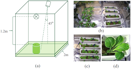
Fig. 1. Collection and production process of the pak choi dataset. (a) is the internal layout of the dual camera incubator. The original camera image is shown in (b). This image undergoes perspective transformation to produce (c), which is cropped to obtain the single-plant image in (d).
Table 2. Datasets summary statistics.

A camera with a resolution of \(1920 \times 1080\) pixels was used to record the complete growth cycle of the pak choi. As shown in Fig. 1(a), the camera was fixed in the middle position above the incubator, one at the front and one at the back, and the lens was shot at a perpendicular distance of 1.2 m from the target leaves, skewed downward by 45°. The photographing interval was 4 h 9.
An image of the pak choi growth process is shown in Fig. 1(b). First, the top view was restored by perspective transformation, and an image was obtained, as shown in Fig. 1(c), which was used to produce the growth stage dataset of pak choi (GS-PC). Based on experimental requirements and the standardized BBCH scale, we categorized the pak choi growth process into three primary stages: germination, seedling, and vigorous growth 10,11. The germination stage is characterized by a field emergence rate exceeding 10% and the full expansion of cotyledons. The seedling stage was identified by the presence of at least one true leaf, along with a plant height below 7 cm or a total leaf number no greater than nine. Progression into the vigorous growth stage was defined as an average leaf count exceeding nine leaves, accompanied by a marked increase in above-ground dry matter accumulation. This classification scheme provides a clear basis for subsequent quantitative observations and experiments on pak choi growth.
The statistical profiles of the datasets are listed in Table 2. To improve the efficiency of the model training and ensure the accuracy of the training results, the pixel size of the images was uniformly compressed to \(640 \times 640\) pixels.
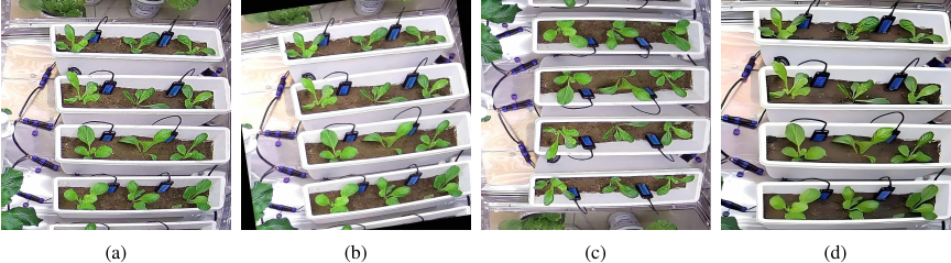
Fig. 2. Data enhancement of pak choi pictures. (a) is the original image. (b) is the image after rotation and brightness enhancement. (c) is a vertical flip of the image, and (d) is the enlarged image.
Table 3. Pearson correlation analysis between total fresh weight and physiological and morphological traits in pak choi.

Owing to the limited and uneven number of collected images of pak choi, as well as the uniform lighting and background, data augmentation processing was performed on the growth images of pak choi to improve model accuracy and robustness. We used a random mixture of techniques such as brightness adjustment (\(\pm10\)%), flipping, angle rotation (\(\pm15{°}\)), and image scaling (up to 15%). The image obtained after data enhancement is shown in Fig. 2. Additionally, the YOLOv5 model utilizes mosaic data enhancement 12, which splices four input images into a single large mosaic image. This approach can effectively simulate the interrelationships and interactions between the backgrounds of pak choi planting in a real scene.
2.2. Feature Selection
To investigate the relationship between the morphological traits and total fresh weight of pak choi, a series of experiments was designed to collect quantitative measurements of chlorophyll content, maximum leaf length, maximum leaf width, average leaf thickness, and total leaf surface area. Pearson correlation analysis was conducted to evaluate the contribution of each morphological feature to the prediction of total fresh weight, as listed in Table 3.
The results showed strong positive correlations (\(p < 0.01\)) between total fresh weight and maximum leaf length (\(r = 0.898\)), maximum leaf width (\(r = 0.813\)), and leaf surface area (\(r = 0.860\)). In contrast, total fresh weight was not significantly correlated with leaf thickness (\(p > 0.05\)). However, further assessment identified strong multicollinearity among the leaf surface area, maximum leaf length, and maximum leaf width. The simultaneous inclusion of these three variables in a regression model results in severe multicollinearity, compromising the stability and interpretability of the regression coefficients. Consequently, leaf surface area was chosen as a representative morphological variable for subsequent modeling.
Chlorophyll content was incorporated as a key predictor. Although chlorophyll content demonstrated a comparatively weaker correlation with total fresh weight, it served as an indicator of photosynthetic capacity and physiological activity, thereby contributing a distinct functional perspective to biomass estimation. This selection effectively avoids multicollinearity when introducing complementary information. The resulting model, which combines leaf surface area and chlorophyll content, integrates both structural and functional traits, and enhances its stability and physiological relevance for predicting the total fresh weight of pak choi.
3. Proposed Methodology
3.1. Total Fresh Weight Estimation Model for Pak Choi
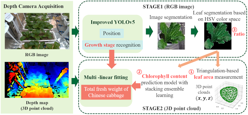
Fig. 3. Flowchart of the quantitative computational modeling of growth states.
This study proposed a quantitative calculation model for the growth status of pak choi, as shown in Fig. 3. A depth camera was used to capture the RGB images and 3D point cloud data of the target scene simultaneously. As a single image contains multiple plants, we used an improved YOLOv5 model based on the ASPP module and Ghost convolution in the first stage to locate individual pak choi plants and identify their growth stages (germination, seedling, and vigorous growth). Based on the localization results, images of individual plants were cropped, as shown in Fig. 1(c). Subsequently, a method based on the HSV color space was used to segment the leaves.
In the second stage, the growth parameters of the pak choi were calculated. Based on the leaf area obtained through segmentation, the corresponding 3D point cloud data, which included the spatial coordinates \((x, y)\) and depth information \(z\), were extracted. After applying SOR filtering to the extracted point cloud, the convex hull algorithm was used to construct a continuous triangular mesh surface from a discrete point cloud. The leaf surface area (\(A_{l}\)) was calculated using the triangular element accumulation method. Simultaneously, the chlorophyll content (\(C_{\mathit{chl}}\)) was predicted from the RGB image of the leaf region using a stacking ensemble model developed for chlorophyll estimation. Considering the issue of leaf occlusion, we added the ratio of image pixels occupied by the leaf surface (\(R_{l}\)) to the independent variables and used multiple linear regression to calculate the total fresh weight of the pak choi.
\(R_{l}\) represents the probability of unidentified leaf presence, derived from the HSV color space-based leaf segmentation. For pak choi at the germination stage (Index1), the ratio was set to 0 due to minimal leaf occlusion. The ratio was calculated based only on the leaf pixel occupancy rate when the growth stage recognition model predicted the seedling (Index2) or vigorous growth (Index3) stages. Let the width of the single pak choi image be \(w\), height be \(h\), and leaf segmentation area region be \(C\). If the growth stage recognition results in \(x\), the formula for the independent variable of the image pixel ratio occupied by the leaf surface is shown in Eq. \(\eqref{eq:Equation1}\).
Finally, we obtained an equation for calculating the total fresh weight of a single pak choi using multivariate linear fitting, as shown in Eq. \(\eqref{eq:Equation2}\).
3.2. Lightweight YOLOv5 Model Based on ASPP Module and Ghost Convolution
Substantial morphological variations during the growth cycle of pak choi, combined with frequent inter-plant occlusion under high-density planting conditions, significantly degrade the detection performance of conventional YOLOv5. Furthermore, the computational constraints of devices in agricultural settings require lightweight architectures for real-time inference. Therefore, this study incorporates Ghost convolutions and ASPP modules into YOLOv5’s Backbone and Neck networks. The proposed modifications enhance multi-scale recognition accuracy while reducing the parameter count and improving computational efficiency 13,14,15.
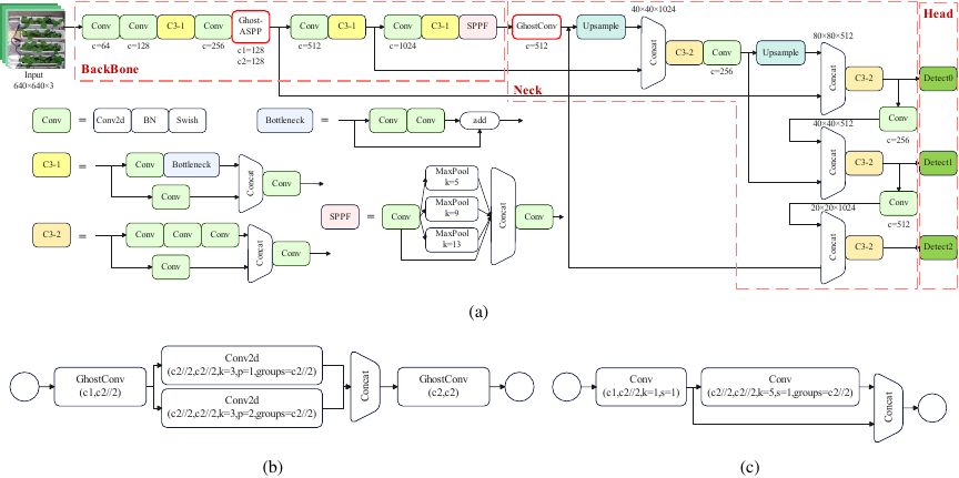
Fig. 4. The framework of improved YOLOv5. (a) is an improved YOLOv5 network architecture that replaces the second C3 module in the Backbone with a Ghost-ASPP module (b) and introduces GhostConv (c) in the first convolutional layer of the Neck to replace the standard convolution.
The improved YOLOv5 network architecture is shown in Fig. 4(a), and the specific improvements are divided into the following two parts:
-
(1)
The second C3 module in the Backbone is replaced with the Ghost-ASPP module, as shown in Fig. 4(b). This module first uses GhostConv to reduce the number of channels, and then employs parallel deep separable convolutions with different dilation rates (dilation rates \(=\) 1, 2) to capture local details and global contextual information, respectively. Finally, the spatial features of different scales are fused through concatenation and GhostConv. This module enhanced the robustness of the model, enabling the effective identification of pak choi at different growth stages.
-
(2)
In the Neck, GhostConv was introduced to replace part of the standard convolution, as shown in Fig. 4(c), which uses linear convolution to reduce the number of model parameters. The Ghost module adopts a dual-path feature generation mechanism. The main path generates a basic feature map through a standard convolution (\(1 \times 1\)), and the number of output channels is compressed to half of the original size. The secondary path applies a \(5 \times 5\) depth-separable convolution to the main path output to generate the remaining channels through an inexpensive linear computation.
3.3. Leaf Segmentation Method Based on HSV Color Space
Leaf image segmentation affects the quality of the subsequent 3D point cloud selection and the accuracy of the total fresh weight calculations. Traditional segmentation methods in the RGB color space are highly susceptible to changes in the light intensity and color temperature 16,17,18. In natural agricultural settings, the chromatic characteristics of leaves exhibit significant variability owing to fluctuating environmental conditions including illumination changes, weather variations, and heterogeneous soil backgrounds. We propose a lightweight leaf segmentation method based on the HSV color space, which improves segmentation quality and robustness while meeting the real-time requirements of monitoring systems.
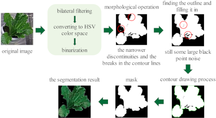
Fig. 5. Flowchart of leaf color segmentation based on HSV space.
A flowchart of the leaf segmentation process image is shown in Fig. 5. First, a bilateral filter is applied to the cropped image to smooth textures and suppress noise, thereby enhancing the subsequent color segmentation. The image is then converted from RGB space to HSV space, and a binary image (mask) is generated by segmenting it according to the green range. The green part is the white pixel and the other colors are black pixels. Next, the segmented binary image is subjected to a closed operation to bridge the narrower discontinuities and fill the breaks in the contour lines making the contours smoother. Subsequently, the processed image was subjected to an open operation to eliminate the white noise and fine parts. Although a more completely segmented image was obtained at this stage, some larger black noise spots remained. Considering the morphological characteristics of pak choi with larger leaves and coarser rhizomes in the late stages of growth, we identified the outline of the plant and filled it internally. Finally, the leaf regions are segmented and isolated from the image.
3.4. Chlorophyll Content Prediction Model with Stacking Ensemble Learning
Based on the methodology of Zhang et al. 19, six color indices (\(B\), GI, GLA, \(g\), \(g - b\), and CIVE) are extracted from the RGB images of segmented leaf regions and selected as feature variables to estimate chlorophyll content, whose definitions are provided in Eqs. \(\eqref{eq:gi}\) to \(\eqref{eq:cive}\). Among these, the \(B\) channel reflects chlorophyll absorption characteristics in the blue spectrum. The GI and CIVE indices enhanced the distinction between vegetation and background, whereas GLA and \(g\) intensified the leaf greenness from different perspectives. The \(g - b\) index highlights chlorophyll-sensitive responses by leveraging the spectral difference between green and blue bands.
Based on the selected features, a stacking ensemble modeling strategy was implemented. At the first level, three base learners, multiple linear regression (MLR), support vector regression (SVR), and random forest (RF), were employed to generate preliminary predictions of chlorophyll content, capturing both linear and non-linear relationships among the multidimensional vegetation indices. At the second level, ridge regression was utilized as the meta-learner, integrating the base learners’ predictions through regularized linear weighting. This design mitigates multicollinearity among the base predictions, resulting in a more stable and robust model for estimating chlorophyll content in pak choi. The ensemble model achieved a coefficient of determination (\(R^2\)) of 0.713 and a root mean square error (RMSE) of 3.094 on the test set, demonstrating strong predictive performance.
3.5. Leaf Surface Area Computation Based on Triangular Mesh Reconstruction
Common surface area calculation methods include planar projection, voxelization, unstructured point cloud integration, and triangular mesh techniques 20,21,22. Because of the curling and wrinkling of leaves, which creates uneven structures, we used the triangular meshing method to construct a continuous surface model using the convex hull algorithm. This can help fully retain the topological structural characteristics of the leaves and reduce surface area calculation errors.

The point cloud extracted from the leaf section was filtered using SOR filtering, followed by surface reconstruction using the convex hull algorithm. The pseudocode for triangular mesh generation is provided in Algorithm 1. Tetrahedra were initially constructed as the basic structure of the convex hull, and the remaining point cloud data were then inserted point by point. For each point to be inserted, the half-edge data structure is iteratively updated through visible face detection. After removing all the visible faces from the current convex hull, a new point was connected to the boundary edges of the visible faces to generate new triangular faces, thereby expanding the convex hull shell. The final convex hull was used to calculate the surface area of the leaves.
After completing the triangular meshing, the surface area of the leaves was calculated by summing the areas of all triangular elements. Specifically, for each triangular element \(\triangle ABC_{i}\), we first calculated the two edge vectors based on the coordinates of the three vertices \(A_{i}(x_{i1}, y_{i1}, z_{i1})\), \(B_{i}(x_{i2}, y_{i2}, z_{i2})\), and \(C_{i}(x_{i3}, y_{i3}, z_{i3})\). The area of a single element is then calculated using the formula for the magnitude of the cross product of the vectors \(S_{\triangle ABC_{i}}\), as follows:
Through Eq. \(\eqref{eq:Equation5}\), the total surface area of the leaves was obtained by accumulating the areas of the triangles.
4. Experimental Results and Analysis
4.1. Evaluation Metrics
This study evaluated the detection results of the improved YOLOv5 model using commonly used target detection evaluation criteria, including precision (P), recall (R), precision–recall curve (PR curve), mean average precision (mAP) for all classes, and the comprehensive evaluation index F1 value. We also evaluated the computational efficiency of the model using frames per second (fps) and related parameters 23,24.
Precision measures the proportion of correctly predicted positive instances among all model-predicted positives, whereas recall indicates the fraction of actual positives correctly identified by the model. Here, \(\mathit{TP}\) denotes correctly detected bounding boxes with an IoU exceeding a specified threshold, \(\mathit{FP}\) represents incorrect positive predictions, and \(\mathit{FN}\) represents undetected ground-truth instances.
A PR curve can be plotted using recall as the \(x\)-axis and precision as the \(y\)-axis. The area under the PR curve was defined as the AP, which was calculated using interpolation, as shown in Eq. \(\eqref{eq:Equation8}\). Calculate the AP for all categories and calculate the average to obtain the mAP, as shown in Eq. \(\eqref{eq:Equation9}\). Assuming that \(K\) categories exist.
The F1 score is a metric for multi-class classification problems that considers precision and recall as equally important. The formula used is as follows:
The evaluation criteria for the multiple linear regression included model fit, regression significance, residual normality, independence, and variance homogeneity. In this study, we used the coefficient of determination, regression significance test (F-test), and Durbin–Watson test (DW test) to evaluate the fitting effect 25,26,27,28.
The coefficient of determination \(R^2\) represents the percentage of variation in the dependent variable, which can be explained by the independent variable, and reflects the accuracy of the regression equation fit. Adjusted \(R^2\) is commonly used in multiple linear regression to offset the impact of sample size. The calculation formula is as follows:
The numerator in Eq. \(\eqref{eq:Equation11}\) represents the sum of the squared differences between the predicted and true values, whereas the denominator denotes the sum of the squared differences between the mean and true values. As expressed in Eq. \(\eqref{eq:Equation12}\), \(n\) is the sample size and \(p\) is the number of features. An increasing magnitude of \(R^{2}\mathrm{{\_}adjusted}\) indicates an improved goodness-of-fit for the regression model.
The F-test is a test of the overall significance for regression models that tests whether the combined effect of all explanatory variables on an explained variable is significant. According to the principles of hypothesis testing, the null and alternative hypotheses were as follows:
The DW test was used to test the independence of residuals in the regression analysis. The residuals \(e\) are the differences between the predicted and actual values in the population. The correlation equation for each residual is \(e_{t} = \rho e_{t-1} + v_{t}\), the null hypothesis \(H_0\) is \(\rho = 0\), and the statistical formula is given by Eq. \(\eqref{eq:Equation15}\).
As \(d \approx 2(1-\rho)\), \(d\) closer to 2 indicates better residuals. Generally, \(d\) between 1 and 3 indicates that the regression meets the residual independence test.
Table 4. Hyperparameter setting and fine-tuning.

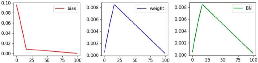
Fig. 6. Learning rate change strategies for training.
Table 5. Experimental environment configuration for the YOLOv5 network model.

Table 6. Ablation test results for the improved YOLOv5 model.

4.2. Training Details
In this study, YOLOv5 was used for localization and growth stage identification of pak choi. The hyperparameters and hyperparameter fine-tuning methods that we set during the model training are listed in Table 4. The learning rate is adjusted through LambdaLR, as shown in Fig. 6. The initial learning rate of the bias layer is 0.1 to ensure faster adjustment. Here, we used a warm-up learning strategy in which the learning rate increased linearly from a smaller value to the initial learning rate within the warm-up phase, and then decayed linearly.
This study was conducted on a computing platform equipped with an Intel Xeon Platinum 8352V CPU and an NVIDIA RTX 4090 GPU. The environment was built on Ubuntu 20.04, and PyTorch 1.11.0 was utilized for deep neural network implementation, with the detection environment including CUDA 11.3 and Python 3.8 (see Table 5).
4.3. Analysis of improved YOLOv5
To validate the effectiveness of the model improvements, we conducted ablation experiments on the improved parts and compared the experimental results, as listed in Table 6. The same hyperparameters and preprocessing operations were used in the experiments to ensure methodological rigor and reproducibility.
The ablation experiment results showed that compared with the baseline model YOLOv5s, introducing the Ghost-ASPP module alone resulted in a slight improvement in P (0.9%) and R (0.9%), with the mAP and F1-score increasing by 1.8% and 1.98%, respectively, and a slight improvement in inference speed. This indicates that the Ghost-ASPP module enhances the feature extraction capabilities while reducing the number of computational parameters and improving the computational efficiency. When only the GhostConv module was used to replace standard convolutions, compared to the baseline model, YOLOv5+GhostConv achieved improvements of 3.4%, 2.5%, 3%, and 3.57% in P, R, mAP, and F1-score, respectively, with a slight increase in inference speed to 120.62 fps. The number of parameters is reduced by 300,416, indicating that the GhostConv module effectively reduces the feature map redundancy and improves the detection accuracy.
The joint model combining the Ghost-ASPP and GhostConv modules achieved the best performance, with P, mAP, and F1-score reaching the highest values, representing increases of 5.9%, 3.5%, and 4.66%, respectively, compared to YOLOv5s. It also maintained a high recall rate. Owing to the parallel structure of the Ghost-ASPP module and the inexpensive linear operations of the GhostConv module, the computational load of the model was significantly reduced, achieving a real-time inference speed of 121.54 fps, an increase of 2.31 compared to the baseline model.
It can be observed that there is a synergistic effect between the Ghost-ASPP and GhostConv modules. Ghost-ASPP enhances multi-scale feature representation capabilities, whereas GhostConv optimizes computational efficiency by reducing redundant features. Both improve the accuracy of identifying the growth stages of pak choi while reducing the number of model parameters and improving computational efficiency.
To fully illustrate the applicability of the proposed model, Fig. 7 shows the recognition results of the baseline model YOLOv 5s and the improved model. It can be observed that the improved model has a higher recognition accuracy for pak choi at different growth stages.
4.4. Results from Fitting the Total Fresh Weight Equation
This study conducted fitting experiments using two variables (\(A_{l}\), \(C_{\mathit{chl}}\)) and three variables (\(A_{l}\), \(C_{\mathit{chl}}\), \(R_{l}\)), and the fitting performances are listed in Table 7. The results indicated that incorporating \(R_{l}\) as an additional independent variable improved the overall model fit, reducing the mean relative error to 12.16%. In this case, the coefficient of determination (\(R^2\)) reached 0.790, suggesting that the predictors collectively explained 79% of the variation in total fresh weight, which aligned with our expectations. The DW test result was \(d = 1.742\), which fell between 1 and 3, indicating that the independence of the fitting residuals was satisfied.
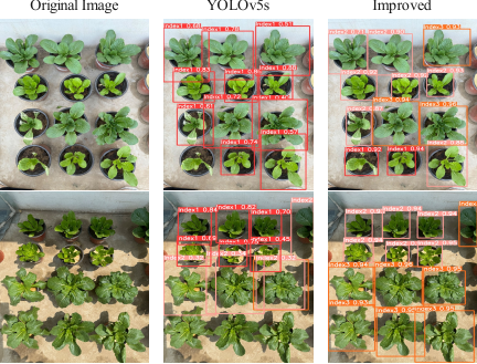
Fig. 7. Comparison of detection results using baseline and improved YOLOv5
Table 7. Model fit summary.

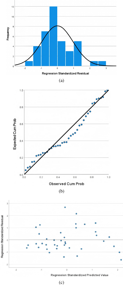
Fig. 8. Residual testing. (a) Histogram of the standardized residuals. (b) Normal probability plot showing the relationship between cumulative frequency distribution and theoretical distribution. (c) Scatter plot showing the characteristics of the residual distribution.
Table 8. Results of regression analysis.

The residuals were then tested. As shown in Fig. 8(a), the mean of the standardized residuals is \(\mbox{$-$1.98E-15} \approx 0\), and the standard deviation is 0.96, which is close to 1. The residuals follow a normal distribution, meeting the normality condition for linear regression. The normal probability plot (P-P plot) of the standardized residuals, shown in Fig. 8(b), is approximately a straight line, indicating conformity with a normal distribution. The standardized residual plot shown in Fig. 8(c) indicates that the residual scatter points were distributed around zero, maintaining an approximately symmetrical distribution without significant changes as the predicted values increased. This indicated that the residuals of the linear regression model for total fresh weight of pak choi met the conditions of homoscedasticity and independence.
The results of the analysis of variance showed that when \(\mathrm{F} = 42.601\), \(p < 0.001\). This indicates that at least one independent variable affects the dependent variable, thereby increasing the regression variance and reducing the residual variance; the model passes the overall significance test.
The regression coefficients were calculated, and significance and multicollinearity tests were performed, as listed in Table 8. It can be observed that the independent variables \(A_{l}\) (\(t = 7.648\), \(p < 0.001\)) and \(C_{\mathit{chl}}\) (\(t = 2.394\), \(p = 0.022\)) have statistically significant effects on the total fresh weight of pak choi, which aligns with practical expectations. Although \(R_{l}\) was not statistically significant, its inclusion in the model, as listed in Table 7, contributed to a reduction in the prediction error and an overall improvement in the model performance. This suggests that \(R_{l}\) provides meaningful information for estimating the total fresh weight of pak choi. The collinearity statistics included two indicators: the variance inflation factor (VIF) and tolerance. Table 8 shows that all variables have \(\textrm{VIF} < 10\) (\(\textrm{tolerance} > 0.1\)), indicating no significant multicollinearity among the independent variables. Therefore, the linear regression model was valid.
The final fitted equation for calculating the total fresh weight of pak choi is expressed in Eq. \(\eqref{eq:Equation2}\).
5. Conclusion
To enable the non-contact measurement of quantitative growth parameters in herbaceous plants, this study proposes a method based on an improved YOLOv5 algorithm combined with 3D point cloud technology to establish a computational model for estimating total fresh weight, with pak choi as the exemplar crop. Considering the requirements for both recognition accuracy and computational speed, the following improvements were made to YOLOv5. (1) Replacing some C3 modules in the Backbone with Ghost-ASPP modules to enhance multi-scale spatial feature extraction and better adapt to the significant size variations of pak choi across different growth stages. (2) Introducing GhostConv to replace some standard convolutions in the Neck by utilizing linear convolutions to reduce the number of model parameters. The experimental results demonstrate that these improvements enhance both detection accuracy and efficiency.
Improved YOLOv5 was used to locate individual pak choi plants and identify their growth stages. After segmenting the images of individual plant, a method based on the HSV color space was used to segment the leaves and extract the corresponding 3D point cloud data. A convex hull algorithm was used to construct a triangular mesh to calculate the leaf surface area. A stacking ensemble model was employed to predict chlorophyll content. Leaf surface area, mean leaf chlorophyll content, and leaf pixel ratio in the images were selected as independent variables. A multiple linear regression model was subsequently developed by integrating these variables with plant’s growth stage to estimate the total fresh weight of pak choi. Consequently, the pak choi fresh weight estimation model demonstrates a favorable balance between predictive accuracy and computational efficiency.
Future work will focus on expanding the dataset to real field cultivation scenarios, including diverse lighting conditions, varying degrees of occlusion, and the presence of other herbaceous species. Additional morphological and phenotypic features will be incorporated to enhance the robustness and generalization capabilities of the model. Simultaneously, more accurate and detailed 3D leaf reconstruction methods will be developed to capture the fine structural characteristics of leaves, thereby improving the precision and applicability of the model to realistic agricultural environments.
- [1] T. Fujinaga, S. Yasukawa, and K. Ishii, “Tomato growth state map for the automation of monitoring and harvesting,” J. Robot. Mechatron., Vol.32, No.6, pp. 1279-1291, 2020. https://doi.org/10.20965/jrm.2020.p1279
- [2] D. Lo Presti et al., “Plant growth monitoring: Design, fabrication, and feasibility assessment of wearable sensors based on fiber bragg gratings,” Sensors, Vol.23, No.1, Article No.361, 2023. https://doi.org/10.3390/s23010361
- [3] S. Joshi, T. R. Naik, R. Patkar, and M. S. Baghini, “Stomatal transpiration monitoring using a wearable leaf sensor,” 2020 IEEE Int. Conf. on Flexible and Printable Sensors and Systems, 2020. https://doi.org/10.1109/FLEPS49123.2020.9239465
- [4] S. Yulianto et al., “Spatial distribution of paddy growth stage using Sentinel-1 based on cart model,” 2021 IEEE Asia-Pacific Conf. on Geoscience, Electronics and Remote Sensing Technology, pp. 73-77, 2021. https://doi.org/10.1109/AGERS53903.2021.9617317
- [5] C.-Y. Song et al., “Detection of maize tassels for UAV remote sensing image with an improved YOLOX Model,” J. of Integrative Agriculture, Vol.22, No.6, pp. 1671-1683, 2023. https://doi.org/10.1016/j.jia.2022.09.021
- [6] S. Zhu, H. Qu, Q. Xia, W. Guo, and Y. Guo, “Parametric reconstruction method of wheat leaf curved surface based on three-dimensional point cloud,” Smart Agriculture, Vol.7, No.1, pp. 85-96, 2025 (in Chinese). https://doi.org/10.12133/j.smartag.SA202410004
- [7] M. Fu et al., “Comparative transcriptome analysis of purple and green flowering Chinese cabbage and functional analyses of BrMYB114 gene,” Int. J. of Molecular Sciences, Vol.24, No.18, Article No.13951, 2023. https://doi.org/10.3390/ijms241813951
- [8] F. Damayanti, S. Yudha S., and A. Falahudin, “Oil palm leaf ash’s effect on the growth and yield of Chinese cabbage (Brassica rapa L.),” AIMS Agriculture and Food, Vol.8, No.2, pp. 553-565, 2023. https://doi.org/10.3934/agrfood.2023030
- [9] S. A. Tsaftaris, M. Minervini, and H. Scharr, “Machine learning for plant phenotyping needs image processing,” Trends in Plant Science, Vol.21, No.12, pp. 989-991, 2016. https://doi.org/10.1016/j.tplants.2016.10.002
- [10] U. Meier, “Growth stages of mono- and dicotyledonous plants: BBCH monograph,” Blackwell, 1997.
- [11] J. Zhang et al., “High-throughput phenotyping of Chinese cabbage using multispectral drone imagery and deep learning for morphological, color, and nutritional traits across growth stages,” Scientia Horticulturae, Vol.346, Article No.114172, 2025. https://doi.org/10.1016/j.scienta.2025.114172
- [12] A. G. C. Gonzalez, G. Venture, I. Mizuuchi, and B. Indurkhya, “VGG-16-based map-less navigation architecture with temporal vision mosaic for autonomous ground robots,” Int. J. Automation Technol., Vol.19, No.4, pp. 651-665, 2025. https://doi.org/10.20965/ijat.2025.p0651
- [13] L.-Y. Zhou et al., “Reclining public chair behavior detection based on improved YOLOv5,” J. Adv. Comput. Intell. Intell. Inform., Vol.27, No.6, pp. 1175-1182, 2023. https://doi.org/10.20965/jaciii.2023.p1175
- [14] Z. Li, Y. Zhang, C. Wang, G. Tan, and Y. Yan, “Improved pedestrian detection algorithm based on YOLOv5s,” J. Adv. Comput. Intell. Intell. Inform., Vol.28, No.4, pp. 768-775, 2024. https://doi.org/10.20965/jaciii.2024.p0768
- [15] Q. Zhou and Y. Liu, “RCT-YOLOv8: A tuna detection model for distant-water fisheries based on improved YOLOv8,” J. Adv. Comput. Intell. Intell. Inform., Vol.28, No.6, pp. 1273-1283, 2024. https://doi.org/10.20965/jaciii.2024.p1273
- [16] E. Hamuda, B. Mc Ginley, M. Glavin, and E. Jones, “Automatic crop detection under field conditions using the HSV colour space and morphological operations,” Computers and Electronics in Agriculture, Vol.133, pp. 97-107, 2017. https://doi.org/10.1016/j.compag.2016.11.021
- [17] Q. Lei, J. Liu, M. Wu, and J. Wang, “Image clustering using active-constraint semi-supervised affinity propagation,” J. Adv. Comput. Intell. Intell. Inform., Vol.20, No.7, pp. 1035-1043, 2016. https://doi.org/10.20965/jaciii.2016.p1035
- [18] Q. Chen et al., “Evaluating goji berry (Lycium barbarum L.) quality change during storage using color and fluorescence imaging system,” J. of Food Composition and Analysis, Vol.141, Article No.107342, 2025. https://doi.org/10.1016/j.jfca.2025.107342
- [19] X. Zhang, H. Yu, J. Yan, and X. Meng, “Study on the detection of chlorophyll content in tomato leaves based on RGB images,” Horticulturae, Vol.11, No.6, Article No.593, 2025. https://doi.org/10.3390/horticulturae11060593
- [20] H. Song, W. Wen, S. Wu, and X. Guo, “Comprehensive review on 3D point cloud segmentation in plants,” Artificial Intelligence in Agriculture, Vol.15, No.2, pp. 296-315, 2025. https://doi.org/10.1016/j.aiia.2025.01.006
- [21] N. Yamaguchi, H. Okumura, O. Fukuda, W. L. Yeoh, and M. Tanaka, “Estimating tomato plant leaf area using multiple images from different viewing angles,” J. Adv. Comput. Intell. Intell. Inform., Vol.28, No.2, pp. 352-360, 2024. https://doi.org/10.20965/jaciii.2024.p0352
- [22] G. Zheng and L. M. Moskal, “Computational-geometry-based retrieval of effective leaf area index using terrestrial laser scanning,” IEEE Trans. on Geoscience and Remote Sensing, Vol.50, No.10, pp. 3958-3969, 2012. https://doi.org/10.1109/TGRS.2012.2187907
- [23] D. M. W. Powers, “Evaluation: From precision, recall and F-measure to ROC, informedness, markedness and correlation,” arXiv:2010.16061, 2020. https://arxiv.org/abs/2010.16061
- [24] M. Fang et al., “Small object detection algorithm based on improved attention mechanism and feature fusion of YOLOv8,” J. Adv. Comput. Intell. Intell. Inform., Vol.29, No.4, pp. 941-955, 2025. https://doi.org/10.20965/jaciii.2025.p0941
- [25] N. R. Draper and H. Smith, “Applied Regression Analysis,” John Wiley & Sons, 1998. https://doi.org/10.1002/9781118625590
- [26] J. Neter, W. Wasserman, and M. Kutner, “Applied Linear Statistical Models: Regression, Analysis of Variance, and Experimental Designs,” 3rd Edition, CRC Press, 1990.
- [27] K.-H. Yuan and P. M. Bentler, “ F F tests for mean and covariance structure analysis,” J. of Educational and Behavioral Statistics, Vol.24, No.3, pp. 225-243, 1999. https://doi.org/10.3102/10769986024003225
- [28] C. Wang, “Expectation and variance of Durbin Watson test statistic DW,” J. of Yanan University (Natural Science Edition), Vol.14, No.3, pp. 38-41, 1995 (in Chinese).
This article is published under a Creative Commons Attribution-NoDerivatives 4.0 Internationa License.