Research Paper:
Reinforced Optimization: An Objective-Based Optimization Algorithm for Reinforcement Learning
Ali Ridho Barakbah†
 , Irene Erlyn Wina Rachmawan, Ira Prasetyaningrum
, Yuliana Setiowati
, and Weny Mistarika Rahmawati
, Irene Erlyn Wina Rachmawan, Ira Prasetyaningrum
, Yuliana Setiowati
, and Weny Mistarika Rahmawati
Politeknik Elektronika Negeri Surabaya
Jl. Raya ITS, Sukolilo, Surabaya 60111, Indonesia
†Corresponding author

Reinforcement learning (RL) is a machine learning paradigm that enables systems to learn from experience within uncertain environments. However, RL is typically suited to goal-oriented problems rather than objective-driven tasks. To address this limitation, this paper proposes a new optimization algorithm, called reinforced optimization (RO). This algorithm leverages an RL framework and reformulates it from a goal-based setting into an objective-based formulation, enabling its application to optimization problems. The algorithm preserves essential RL elements such as rewards and penalties, as well as exploration and exploitation mechanisms. It utilizes sequences of rewards to represent problem states and updates these states through directional steps. The effectiveness of each action with respect to the objective function is evaluated: successful actions lead to increased rewards, while unsuccessful actions result in decreased rewards. This iterative process continues for a predefined number of iterations, aiming to achieve convergence towards a global optimum in optimization tasks. To evaluate the RO algorithm, experiments were conducted on three objective-based problems: centroid optimization, traveling salesman problem, and vehicle routing problem. The algorithm’s performance was compared to other optimization methods: genetic algorithm, ant colony optimization, simulated annealing, and particle swarm optimization. The results indicate that the RO algorithm exhibits behavior analogous to gradient descent during convergence and demonstrates a favorable trade-off between accuracy and execution time, making it a viable alternative for both continuous and combinatorial optimization problems.
Reinforced optimization
1. Introduction
A recent learning theory, developed by many scientists, is based on supervised learning. In supervised learning, a machine learning algorithm learns to infer a function from labeled training data. By analyzing these data, the algorithm generates a function that can be used to make predictions on new, unseen inputs. However, this approach does not create a truly self-improving learning machine. Instead, it results in a trained or “smart” machine that performs well only after a specific training process.
Reinforcement learning (RL) is a learning paradigm that is applied to a machine or computer system to create a smart machine. Inspired by behaviorist psychology, RL concerns how a software agent should take action in an environment and collect as many rewards as possible to reach its goal 1,2. The agent decides which action to take by considering exploitation and exploration. Exploitation is the process of obtaining as much information as possible from one’s existing knowledge or experience. Exploration is the process of collecting new information from an environment by exploring a previously defined state within that environment 3.
RL combines supervised and unsupervised learning theory, which makes it interesting because it learns and becomes more intelligent through interaction with its environment 4. RL improves the agent’s ability to solve a problem by collecting rewards at each step. Thus, RL is a learning paradigm that enables machines to become smarter through autonomous learning 5.
The literature on objective-based optimization, also known as function-based optimization, is also extensive. This particular objective-based problem and its various adaptations are employed across numerous resource management domains, including, but not limited to, cargo loading, industrial production, menu optimization, and resource distribution within multimedia servers. Until recently, precise methodologies for addressing objective-based (function-based) optimization issues have been largely supplanted by metaheuristic techniques that generate solutions using stochastic numerical values across multiple states, as exemplified by genetic algorithm and ant colony optimization 6. The stochastic nature of these numerical values results in divergent solutions across different experimental iterations.
RL algorithms enhance an agent’s ability to solve problems effectively. RL is a relatively recent problem-solving paradigm inspired by human brain functions. Specifically, the brain learns by exploring new situations and storing outcomes as rewards 7. The human brain also learns through experience by exploiting known conditions. Consequently, RL has become a highly successful subfield of artificial intelligence. RL is particularly valuable for solving a wide range of problems for which models are not known in advance, as many RL algorithms have proven to converge to an equilibrium. However, this convergence is typically limited to goal-based problems rather than objective-based problems.
RL is inherently designed for goal-based problems because its framework focuses on learning how an agent takes actions in an environment to optimize a cumulative reward signal to achieve a goal, rather than learning a direct mapping from inputs to outputs, as in objective-based problems. While objective-based problems focus on optimizing a measure of quality or efficiency, enabling evaluation by degree, goal-based problems focus on achieving a specific, predefined outcome and use a binary measure of success (achieved or not). In RL, an agent interacts with its environment over a sequence of time steps. The agent’s behavior is guided toward a long-term goal through the feedback received in the form of rewards or penalties. In RL, goal-based problems frequently involve a sequence of correct actions to achieve the final outcome. RL excels at this by evaluating actions based on their expected future rewards. The success of RL in goal-based problems is binary (success or failure), whereas the success in objective-based problems is graded (real numbers) and measured by how well the objective function is optimized, such as improved precision, reduced error, lower computational cost, increased certainty, or simpler parametrization. RL is therefore well suited to goal-oriented tasks, as it effectively addresses uncertainty, accommodates delayed rewards, and acquires optimal behavior through direct interaction with the environment, beyond the limitations of conventional supervised function approximation. Therefore, in this study, we propose a new algorithm to apply RL to objective-based optimization problems.
2. Basic Concept of Reinforcement Learning
RL is a method used to train an agent by allowing it to learn from experience 8. The agent receives rewards based on its actions and uses this feedback to guide future decisions. Rather than focusing solely on immediate rewards, the agent aims to maximize the total reward over time. To achieve this, it typically interacts with the same environment repeatedly, gradually learning which actions lead to the most favorable long-term outcomes.
Balancing exploitation and exploration is a critical aspect of RL. Exploitation involves using knowledge from the agent’s existing experience or memory to choose actions that are expected to yield high rewards. In contrast, exploration is the process of gathering new information by interacting with different states in the environment. A distinctive feature of RL, compared to other learning methods, is its use of evaluative feedback. This feedback is assigned to each state based on the agent’s experience and is later used during exploitation to guide future decisions. To generate meaningful evaluation feedback, the agent must actively explore various paths in the environment to identify the most optimal states.
The agent may have found a good goal on one path, but there may be an even better one on another path 9. Without a systematic exploration strategy, the agent invariably reverts to its initial goal, thereby failing to identify potentially superior objectives. Alternatively, the optimal goal may be situated in areas characterized by minimal rewards, which the agent would consciously avoid in the absence of exploration. Conversely, excessive exploration by the agent may hinder its ability to adhere to a designated path; indeed, such behavior reflects a lack of genuine learning, as it becomes incapable of leveraging its accrued knowledge and thus behaves as if it possessed no information whatsoever. Therefore, it is essential to create a prudent balance between exploration and exploitation to ensure that the agent successfully develops the ability to perform optimal actions 10.
The basic scenario in RL aims to maximize cumulative reward 11. This reward signal acts as the primary feedback mechanism, in which the system defines specific rewards for desirable outcomes and penalties for unfavorable ones. A reward or penalty is defined by the RL system. Each optimization case has a different rule for determining the rewards and penalties assigned to the RL agent 12. The output is an action that the agent will take to solve the problem, considering the entire problem using a goal-directed approach.
RL allows an agent to interact with an uncertain environment and learn how to map states to actions to maximize numerical rewards. Unlike traditional machine learning methods, in which correct actions are provided, an agent must discover the most rewarding actions through trial and error. The decision-making process is guided by a policy, which is a function that determines the actions to be taken and is learned over time through the agent’s repeated interactions with its environment 13.
3. Our Proposed Reinforced Optimization Algorithm
The proposed RO algorithm is based on the fundamental principles of RL. In practice, it mirrors the behavior of traditional RL by balancing the exploration of new possibilities and the exploitation of existing knowledge to find optimal solutions. Similar to RL, RO incorporates a reward-and-penalty mechanism in which the agent learns to maximize cumulative reward over the learning process. Rewards and penalties are assigned by the environment based on the actions of the agent. In RO, the policy is learned through trial and error. At each step, the agent observes the current state of the environment, selects and executes an action that modifies the environment, and receives a scalar feedback signal \(r\) (either a reward or a penalty).
RO offers advantages in solving optimization problems by applying an intelligent learning-based approach based on RL principles. By incorporating the core characteristics of RL, the algorithm enables experience-driven learning aimed at achieving a global optimum.
3.1. Originality
This paper presents a novel optimization algorithm, called reinforced optimization (RO). This proposed algorithm employs an RL framework and transforms it from a goal-oriented to an objective-oriented formulation, thereby facilitating its application to optimization problems. The proposed RO algorithm incorporates two fundamental principles of RL: (1) reward and penalty, and (2) exploration and exploitation, which are used to address optimization problems and promote convergence toward a global optimum.
3.2. Variables of Reinforced Optimization
RO is fundamentally based on RL principles. Several variants of the algorithm can be introduced, where \(\beta\) is a variable that influences the magnitude or direction of the agent’s next step, and \(\mu\) is a parameter used to adjust the step value relative to the most recent action.
In RO, the objective of the agent is to learn the optimal solution by updating its action as action \(\leftarrow\) \(d_p\cdot\textit{step}_p\), where the action is accumulated from the previous step and the intended direction \(d\).
The direction \(d\) is a binary value, either \(+1\) or \(-1\), that determines the direction of the value change for the new state. During initialization, \(d\) is set to \(+1\). It is updated in the opposite direction under two conditions:
-
(1)
The new state is worse than the current state.
-
(2)
The new state is identical to the current state, so that the opposite direction will make a greedy movement to allow exploration.
The current state is stored in the variable newS, which is updated by combining the current state and computed action, as described in Eq. \(\eqref{eq:1}\).
The RL technique is well known for using a strategy to learn an optimal policy by learning action values. It iteratively approximates new states. In RO, the action value can be obtained from the direction and the changing step value, which is defined in Eq. \(\eqref{eq:2}\). The step decreases with each iteration to allow larger exploration in the early stages and gradual reduction during the optimization process.
The concepts of exploration and exploitation in RO are used to determine the position of the selected state, either from the state with the largest reward \(r_{\mathit{max}}\) or randomly, depending on the greedy rate. The basic variables of RO are described as follows:
-
State (\(S\)): a finite set of states.
-
Reward (\(r\)): a variable used to assign rewards or penalties.
-
Direction (\(d\)): the direction that guides the agent toward the optimal solution.
-
Step (\(\mathit{step}\)): a variable value for updating the states.
-
MinVal (\(\mathit{minval}\)): the minimum value of states.
-
MaxVal (\(\mathit{maxval}\)): the maximum value of states.
-
\(n\): the number of states.
-
\(\mu\): the learning rate for updating states.
-
\(\beta\): the learning rate for updating rewards.
-
Greedy rate: the rate of exploration.
-
State value (\(\mathit{sv}\)): the value of a state.
-
New state value (\(\mathit{new{\_}sv}\)): the value of a new state.
The state represents the initial position of the agent during the problem-solving process. Depending on the specific case, the state can be initialized with either a predefined value or a random number. The reward variable is used to store the reward associated with each state, typically stored in an array. To control the movement of the agent, a direction variable is defined, which can be set to a positive value to move the agent along the positive axis of the grid. The step value determines how the state is updated and is constrained within a specified range between minval and maxval. These variables are designed to be compatible with optimization problems, and adjustments to the heuristic model may require modifications to the definition or management of the state and direction.
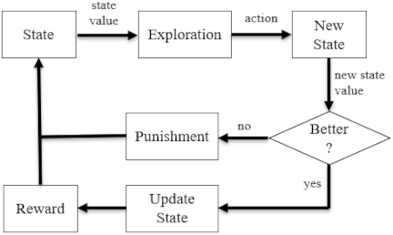
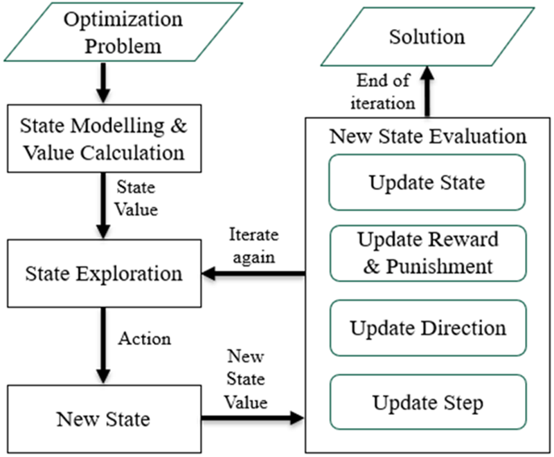
Fig. 1. Computational cycle of the RO.
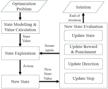
Fig. 2. Overview of the RO algorithm.
3.3. Computational Algorithm
The computational cycle of RO is shown in Fig. 1, which illustrates the flow of RO as it finds the best solution to the optimization problem.
The sequential process of RO is outlined as follows. The algorithm begins by modeling the initial state and calculating its corresponding value. The agent then explores the finite problem environment guided by a predefined exploration rate. If a randomly generated number is greater than the exploration rate, the agent randomly selects a solution within the environment. Conversely, if the random number is less than or equal to the exploration rate, the agent chooses an action based on current reward values. After executing the action, the agent updates its state and recalculates the value of the new state. This value is interpreted as either a reward or a penalty that influences the agent’s subsequent direction of exploration. If the agent receives a penalty, it adjusts its direction accordingly in the next step. This process is repeated for a predefined number of iterations, which is defined as the learning duration of the RO agent. Fig. 2 presents an overview of the RO algorithm.
An extension of this algorithm is presented, in which a parameter is adaptively updated during the execution of the algorithm. Algorithm 1 denotes the computational step of the RO algorithm.

RO begins by initializing the dataset to define the problem environment. The starting position of the agent can be assigned either randomly or based on predefined values, depending on the specific case. After calculating the initial state value, the algorithm decides whether to explore new actions or exploit existing knowledge. It then performs the selected action, updates the state, and calculates the reward based on the new state value. The reward for the new state in the environment is computed using Eq. \(\eqref{eq:3}\).
Equation \(\eqref{eq:3}\) expresses the formula for increasing the reward value when the new state yields a better value. In the case of a penalty, when the new state is worse than the current state, the reward value decreases according to Eq. \(\eqref{eq:4}\).
4. Experimental Study
To evaluate the applicability of the proposed RO algorithm, a series of experiments was conducted on three objective-based problems: centroid optimization, traveling salesman problem, and vehicle routing problem. The performance of RO was compared with other well-known optimization algorithms: genetic algorithm (GA), ant colony optimization (ACO), simulated annealing algorithm (SA), and particle swarm optimization (PSO). Because there are many improved versions of the compared algorithms (GA, ACO, SA, and PSO), the original versions of the compared algorithms were used for the experimental study. The experiments were conducted in MATLAB on a system equipped with an Intel® Xeon® Silver 4114 CPU @2.20 GHz, 64 GB RAM, an Nvidia Quadro P2000 graphics card (5 GB), and a 64-bit operating system running on an x-64-based processor.
4.1. Compared Algorithm
4.1.1. Genetic Algorithm
GA is a search method inspired by the principles of natural evolution. It is commonly applied to find effective solutions for optimization and search problems using mechanisms such as inheritance, mutation, selection, and crossover, which mimic evolutionary processes 14.
In GA, a population of candidate solutions, called individuals, is evolved to find better solutions to an optimization problem. Each individual is represented by a set of characteristics known as chromosomes, which can be modified through mutation and other genetic operations 15.
The evolutionary process typically begins with a population of randomly generated individuals and proceeds iteratively: each iteration is referred to as a generation. In each generation, the fitness of each individual is assessed based on the objective function of the optimization problem. Individuals with higher fitness are probabilistically selected from the current population, and their genetic information is altered to create a new generation. This new generation serves as the population for the next iteration. The algorithm typically stops when either a predetermined maximum number of generations is reached or the population achieves a satisfactory level of fitness 16.
After defining the genetic representation and fitness function, GA begins by initializing a population of solutions. It then iteratively improves this population by applying genetic operators such as mutation, crossover, inversion, and selection. The algorithm consists of two main components: the initialization phase and the iterative process of applying these operators until a satisfactory solution is obtained.
4.1.2. Ant Colony Optimization
ACO is an algorithm inspired by the behavior of ants in nature. Ants move randomly and, when they discover food, return to their colony, leaving behind pheromone trails 17. When other ants encounter a pheromone trail, they tend to follow it rather than wandering randomly. If they also find food, they reinforce the trail by laying down more pheromones 18.
Over time, the pheromone trails naturally evaporate, weakening their attractiveness. The longer it takes an ant to travel along a path and return, the more the pheromone concentration diminishes. In contrast, shorter paths are traversed more frequently, resulting in higher concentrations of pheromones on these routes. This evaporation process helps prevent the algorithm from prematurely converging to a local optimum. Without evaporation, the paths first discovered by the ants would become overly attractive, thereby limiting the exploration of other potential solutions in the search space.
Therefore, when an ant discovers a short and efficient path from the colony to a food source, other ants are more inclined to follow that path. This positive feedback loop eventually causes all ants to converge on the same path. ACO algorithm imitates this natural behavior by having simulated ants explore a graph that represents the problem to be solved 19.
ACO builds solution paths step by step by adding components to the current state. It tracks the transitions observed between pairs of solution components and assigns a desirability value to each transition based on the quality of the solutions in which they appear.
4.1.3. Simulated Annealing
SA is a metaheuristic algorithm designed to find a near-optimal solution to global optimization problems within large search spaces 20. This approach is frequently applied to problems involving discrete search spaces. In some cases, it can be more efficient than exhaustive search methods, particularly when the objective is to find a reasonably good solution within a limited time rather than the absolute best solution 21.
The name and concept of SA are inspired by the annealing process in metallurgy, where a material is heated and then slowly cooled to enlarge its crystal structure and minimize defects, both of which are influenced by the thermodynamic free energy 20. Heating and cooling a material influence both its temperature and thermodynamic free energy. Although the temperature is decreased by the same amount during cooling, the reduction in free energy varies depending on the cooling rate, with slower cooling resulting in a greater decrease in the thermodynamic free energy 22.
In SA, the concept of slow cooling is reflected in the gradual reduction in the probability of accepting worse solutions during the search process. This controlled acceptance of inferior solutions is a key feature of metaheuristic algorithms because it enables a broader exploration of the solution space and helps avoid becoming trapped in local optima.
4.1.4. Particle Swarm Optimization
PSO solves optimization problems using a population of candidate solutions, known as particles, that navigate the search space based on simple mathematical equations that update their positions and velocities 23. Each particle adjusts its movement based on its own best-known position and is influenced by the globally best-known positions found by the swarm. As particles discover better solutions, their positions are updated, guiding the entire swarm toward increasingly optimal solutions 24.
PSO was originally inspired by the social behavior observed in bird flocks and fish schools. The algorithm originated as a simplified model of this movement and was later found to be effective for solving optimization problems 25. PSO is a flexible algorithm that makes minimal assumptions about the nature of a problem and is capable of exploring large solution spaces. However, like other metaheuristic methods, PSO does not guarantee a global optimal solution. Unlike traditional optimization techniques such as gradient descent or quasi-Newton methods, PSO does not rely on gradient information, making it suitable for problems that are non-differentiable, noisy, irregular, or time-varying.
4.2. Experiment in Centroid Optimization
Table 1. Characteristics of datasets used for the centroid optimization problem.

Centroid optimization involves determining the initial starting points or centroids for \(k\)-means clustering. The quality of the final clusters depends heavily on the initial seeds. A common drawback of \(k\)-means is that poor initial centroids cause the algorithm to converge to a local minimum 26. To prevent convergence to a local minimum, the initial centroids are optimized by selecting them to be as far apart as possible. The selection of these starting points significantly influences the clustering process and its outcomes 27. Next, each data point is evaluated by measuring its distance to all cluster centers, and is assigned to the cluster whose center is closest to it 28.
After all the points assigned, a new centroid is calculated for each cluster by averaging the coordinates of the points within that cluster. These mean values represent the coordinates of the updated cluster centers. The assignment step is repeated with the updated centroids in place.
Through this iterative process, the \(k\) centroids gradually shift their positions until they stabilize and no longer change. When the centroids stop moving, or the clustering error no longer decreases, the algorithm reaches a minimum. To optimize the centroid positions, this study uses the sum of squared error (SSE) as a measure, aiming to position the centroids to minimize the SSE 29.
In this experimental study, four benchmark datasets from UCI Repository were used, namely, Iris, Ionosphere, Wine, and Heart datasets, with various characteristics, as shown in Table 1.
For the experiments, the parameters for each algorithm were specified. For the GA, we set a population size of 10, roulette wheel selection, a cross-over probability of 0.9 using a two-point crossover operator, a mutation probability of 0.2 using uniform mutation, and elitism. For the ACO, we set 10 ants, an evaporation rate of 0.5, and a greedy rate of 0.5. For SA, we set \(T_0=1000\), and a cooling rate of 0.5 using a geometric cooling schedule. For PSO, we set 50 swarm particles, an inertia weight of 0.9, and a cognitive and social coefficient of 1.5. For RO, we set \(\mu=0.1\), \(\beta=0.001\), a greedy rate of 0.9, an initial reward \(r=0.5\), an initial \(d=1\), and an initial step value with random values between minval and maxval. Because each algorithm produces non-unique results, we averaged the outcomes of 10 independent runs, each with a time limit of 20 s. Tables 2–5 show the centroid optimization performance of each algorithm for each dataset, including the SSE and the computational time \(t\) [ms].
For the Iris dataset, our proposed RO algorithm and PSO can achieve the minimum SSE; however, RO requires 940 ms, which is substantially less than the 19680 ms required by PSO. For the Ionosphere dataset, RO achieves the minimum SSE among all algorithms with a computational time of 4720 ms. For the Wine and Heart datasets, PSO achieves the minimum SSE compared with the other algorithms. However, RO produces results that are slightly inferior to those of PSO, but RO requires significantly less computational time.
Table 2. Performance of algorithms for centroid optimization on the Iris dataset.

Table 3. Performance of algorithms for centroid optimization on the Ionosphere dataset.

Table 4. Performance of algorithms for centroid optimization on the Wine dataset.

Table 5. Performance of algorithms for centroid optimization on the Heart dataset.

In this experimental study, we analyzed the convergence behavior of each experiment using gradient descent-like curves, as shown in Figs. 3–6. The proposed RO algorithm exhibits smoother convergence with a faster descent rate, leading to more rapid convergence.
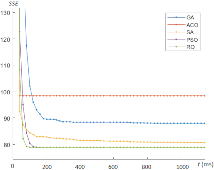
Fig. 3. Convergence behavior for centroid optimization on the Iris dataset.
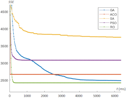
Fig. 4. Convergence behavior for centroid optimization on the Ionosphere dataset.
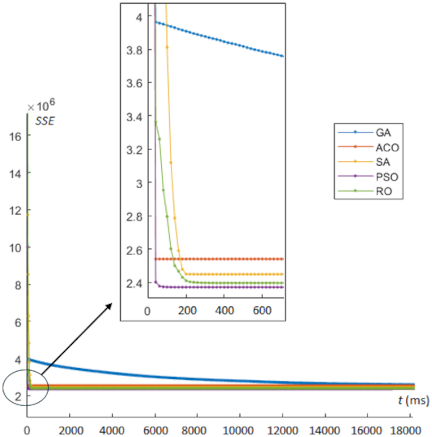
Fig. 5. Convergence behavior for centroid optimization on the Wine dataset.
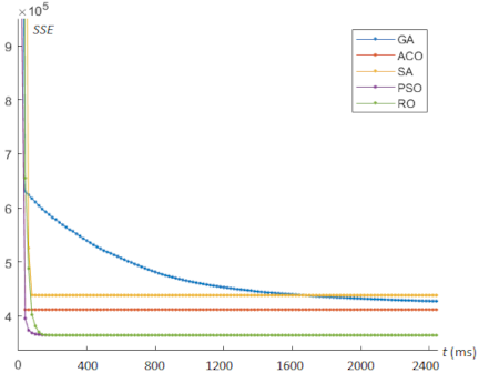
Fig. 6. Convergence behavior for centroid optimization on the Heart dataset.
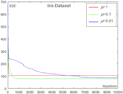
Fig. 7. Convergence behavior showing the effect of the learning rate \(\mu\) on SSE reduction for the Iris dataset.
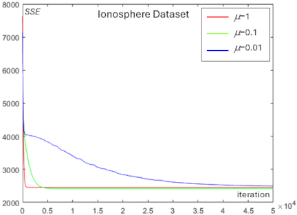
Fig. 8. Convergence behavior showing the effect of the learning rate \(\mu\) on SSE reduction for the Ionosphere dataset.
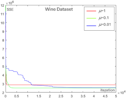
Fig. 9. Convergence behavior showing the effect of the learning rate \(\mu\) on SSE reduction for the Wine dataset.
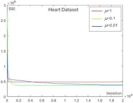
Fig. 10. Convergence behavior showing the effect of the learning rate \(\mu\) on SSE reduction for the Heart dataset.
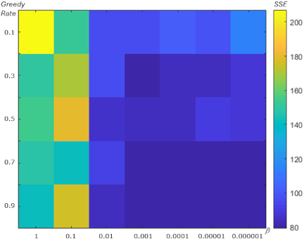
Fig. 11. SSE showing the effect of \(\beta\) and the greedy rate for the Iris dataset.
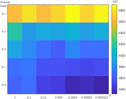
Fig. 12. SSE showing the effect of \(\beta\) and the greedy rate for the Ionosphere dataset.
We analyzed the effect of the learning rate \(\mu\) on the centroid optimization experiments for each dataset. Figs. 7–10 show the convergence behavior resulting from different values of the learning rate \(\mu\) in reducing SSE for the Iris, Ionosphere, Wine, and Heart datasets.
From Figs. 7–10, a higher learning rate \(\mu\) results in a faster initial decrease in SSE; however, it does not converge to the minimum SSE. The largest learning rate with \(\mu=1\) (indicated by the red line), accelerates the reduction of SSE in the early iterations; however, it becomes difficult to reach the minimum SSE in later iterations. In contrast, a moderate learning rate with \(\mu=0.1\) (indicated by the green line) reduces SSE more slowly during the early iterations, but continues to decrease SSE steadily as the iterations progress. However, a very low learning rate, such as \(\mu=0.01\) (indicated by the blue line), slows the descent of SSE considerably and results in higher computational time.
We also analyzed the relationship between the learning rate \(\beta\) and the greedy rate to determine their impact on SSE in the centroid optimization experiments for each dataset. Figs. 11–14 show the SSE values, indicated by color (darker blue indicates lower SSE), as functions of \(\beta\) and the greedy rate.
From Figs. 11–14, the minimum SSE (indicated by the darker blue color) occurs at a greedy rate of 0.9 combined with a lower value of \(\beta\). Across the experiments on the Iris, Ionosphere, Wine, and Heart datasets, as shown in Figs. 11–14, better performance, in terms of lower SSE, is achieved with a higher greedy rate and a lower \(\beta\).
4.3. Experiment in Traveling Salesman Problem
Traveling salesman problem (TSP) is one of the most well-known and challenging computational problems. It involves finding the shortest possible route for a salesperson to visit a set of cities, visiting each city exactly once, and returning to a designated starting city 30. The transportation costs between cities are provided, and the goal is to determine the visiting order that results in the minimum total cost: that is, the most cost-effective route that visits each city once and returns to the starting point 31.
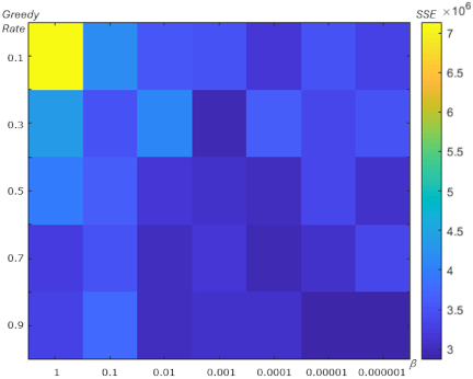
Fig. 13. SSE showing the effect of \(\beta\) and the greedy rate for the Wine dataset.
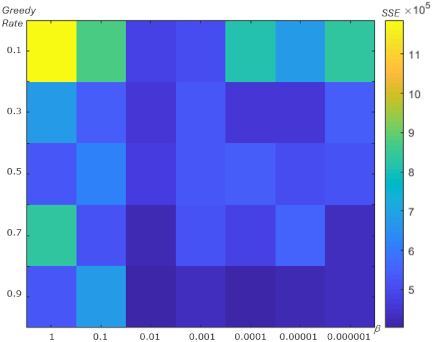
Fig. 14. SSE showing the effect of \(\beta\) and the greedy rate for the Heart dataset.
The algorithm for the standard TSP is described as follows:
-
Initially, all possible solutions are enumerated, which total \((n-1)!\), where \(n\) denotes the number of cities.
-
The cost for each of these \((n-1)!\) solutions is calculated to identify the one with the minimum total cost.
-
Finally, the solution with the lowest cost is selected.
The most common real-world interpretation of the TSP involves a salesperson aiming to find the shortest possible tour through a set of \(n\) clients or cities, represented as nodes. Conceptually, the agent explores all possible paths between nodes, calculates the cost of each path, and identifies the path with the lowest total cost. This process is repeated over a set number of iterations. Once completed, the solution is defined as the path with the minimum total distance, indicating that the optimal route has been found. The TSP is considered a minimization problem, focusing on finding the most efficient route that minimizes the total travel distance.
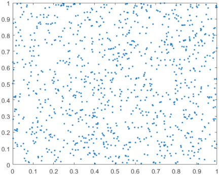
Fig. 15. TSP instance with 1000 nodes (Source: Kaggle, Traveling Salesman Problem by Maxwell).
In this experimental study of the TSP optimization problem, we used a benchmark TSP dataset obtained from Kaggle, namely, Traveling Salesman Problem by Maxwell, which consists of tiny, small, medium, and large instances. For the experiments, we focused on the large instances, using a dataset with 1000 nodes, as shown in Fig. 15.
For the experiments, the parameters for each algorithm were specified. For the GA, we set a population size of 10, tournament selection with a tournament size of 3, a cross-over probability of 0.8 using a two-point crossover operator, a mutation probability of 0.1 with random swap or inversion mutation, and elitism. For the ACO, we set 10 ants, an evaporation rate of 0.8 with \(\alpha=1\), \(\beta=1\), and a pheromone deposit factor \(Q=1\). For the SA, we set \(T_0=1000\), and a cooling rate of 0.8, using a geometric cooling schedule. For the PSO, we set 50 swarm particles, an inertia weight of 0.7, and cognitive and social coefficients of 1.5. For the RO, we set \(\beta=0.001\), a greedy rate of 0.9, an initial reward \(r=0.5\), and an initial direction \(d=1\).
Because the TSP is a combinatorial problem, we slightly modify the proposed RO algorithm to adapt it to this problem through following changes: (1) the reward variable \(r\) is defined as a two-dimensional structure, representing the reward between pairs of nodes; (2) the step component in RO is omitted; and (3) the new state newS is initialized at a random node, and a destination node is selected using a greedy strategy.
Because each algorithm produces non-unique results, we averaged the results over 10 independent runs, each conducted within 3 min (180 s). Table 6 presents the TSP performance of each algorithm with respect to the total tour distance and computational time \(t\) [s].
Table 6. Performance of optimization algorithms for the TSP problem.

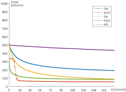
Fig. 16. Convergence behavior for the TSP optimization.
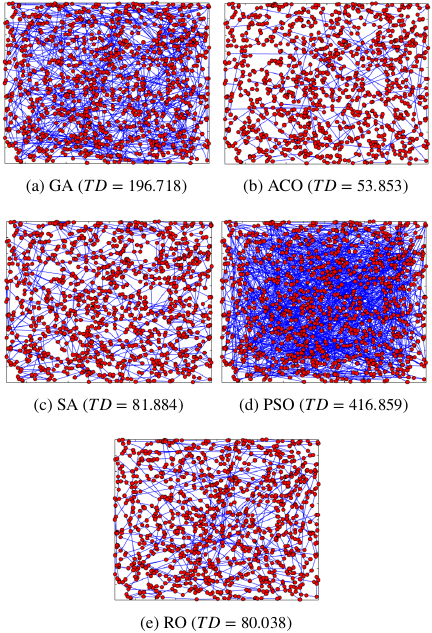
Fig. 17. Visual results of the TSP problem using (a) GA, (b) ACO, (c) SA, (d) PSO, and (e) RO.
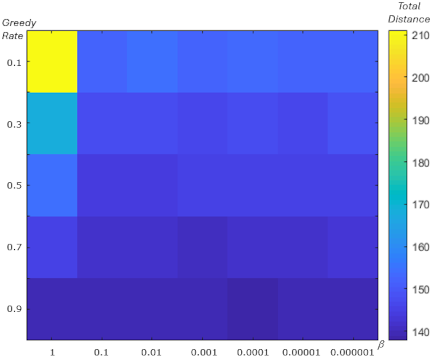
Fig. 18. Total distance showing the effect of \(\beta\) and the greedy rate for the TSP.
Table 6 shows that the proposed RO algorithm is competitive with other optimization algorithms and achieves a minimum distance compared with the other algorithms. However, ACO outperforms RO on this TSP problem, which is expected, as ACO is particularly well suited to the combinatorial problems, such as TSP and VRP 32,33. Moreover, ACO explicitly exploits a precomputed distance metric between nodes to determine transition probabilities during node selection, whereas the other algorithms primarily rely on greedy movement strategies for node selection.
We also analyzed the convergence behavior of the TSP experiment, as shown in Fig. 16. The proposed RO algorithm exhibits smooth convergence with a relatively fast descent rate. Fig. 17 presents visual results obtained using each algorithm for the TSP, indicating that a minimum total distance (\(\mathit{TD}\)) resulted in a slight overlap of lines.
We analyzed the relationship between the learning rate \(\beta\) and the greedy rate to determine their impact on the \(\mathit{TD}\) for the TSP experiment. Fig. 18 shows the \(\mathit{TD}\) values, indicated by color (darker blue indicates lower \(\mathit{TD}\)), as functions of \(\beta\) and the greedy rate. We computed the average \(\mathit{TD}\) from 10 independent runs, each performed with 100000 iterations. From Fig. 18, the minimum \(\mathit{TD}\) (indicated by the darker blue color) occurs at a greedy rate of 0.9 combined with a lower value of \(\beta\), particularly at \(\beta=0.0001\) for a greedy rate of 0.9. Using values of \(\beta<0.0001\) requires substantially higher computational time to further reduce \(\mathit{TD}\). Overall, the results in Fig. 18 indicate that better performance, in terms of lower \(\mathit{TD}\), is achieved with a higher greedy rate and a lower \(\beta\).
4.4. Experiment in Vehicle Routing Problem
Vehicle routing problem (VRP) is one of the most well-known and challenging combinatorial optimization problems. In this problem, an agent must visit \(n\) cities to deliver or collect items while considering the capacity constraints of the vehicle. Each city was visited only once, starting and ending at a central depot. A vehicle can only carry items up to its maximum capacity. The transportation costs between cities are provided, and the goal is to determine the most cost-effective route that completes all deliveries or pickups while minimizing the total travel cost.
The VRP holds a key position in the areas of logistics and physical distribution, where efficient planning of delivery and transportation routes is essential 34. There is a wide variety of VRPs and a broad range of literature on this class of problems. The most common side conditions are as follows:
-
Capacity restrictions: Each city \(i>1\) has an associated non-negative demand \(d_i\), and the total demand served by any vehicle on its route must not exceed its capacity. VRPs with these capacity limits are commonly called capacitated VRPs (CVRPs).
-
The number of cities on any given route is limited to \(q\). This is a specific case of capacity constraints where each city has demand \(d_{i}=1\) for all \(i>1\), and the vehicle capacity is set to \(D=q\).
-
Total time restrictions: The length of any route may not exceed a specified limit \(L\); this length is composed of intercity travel times \(c_{ij}\) and stopping times \(\delta_i\) at each city \(i\) on the route. VRPs with such time or distance constraints are known as distance-constraints VRPs (DVRPs).
-
Time windows: Each city \(i\) must be visited within a specified time frame \([a_{i}, b_{i}]\), and waiting in the city is permitted if the agent arrives earlier than \(a_i\).
-
Precedence constraints between cities: Certain cities must be visited in a specific order, meaning city \(i\) must be visited before city \(j\).
In this experimental study of the VRP optimization problem, we used a benchmark VRP dataset from Kaggle, namely, Solomon VRPTW benchmark by Masud Rahman, which comprises various VRP instances. For the experiment, we used C101 instances from the dataset with 100 nodes, with node \(\ast\) designated as the depot position, as shown in Fig. 19.
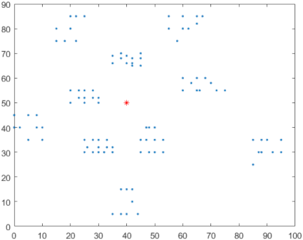
Fig. 19. VRP optimization problem with 100 nodes (Source: Kaggle, Solomon VRPTW benchmark by Masud Rahman).
For the experiments, we set the same parameters for each algorithm in the TSP and applied them to the VRP. Additionally, in this VRP, we set the vehicle capacity to 100, with five vehicles, and \((40,50)\) as the location of the depot (red in Fig. 19). Because each algorithm produced non-unique results, we averaged the results of 10 experiments, each conducted within 1 min (60 s). Table 7 lists the VRP performance of each algorithm in terms of the total distance and computational time \(t\) [s].
Table 7 shows that the proposed RO algorithm achieves the minimum total distance compared to GA, SA, and PSO. Nevertheless, given that ACO is well suited for combinatorial problems such as TSP and VRP, it performs better in this VRP problem 32,33. Furthermore, ACO utilizes a precomputed distance metric between nodes to determine transition probabilities during node selection, whereas the other algorithms employ a greedy approach for this selection process.
We also conducted a convergence analysis for the VRP experiment, as shown in Fig. 20. Our proposed RO algorithm can move smoothly over the execution time to achieve convergence. As shown in Fig. 20, the proposed RO algorithm outperforms the other compared algorithms in the minimization of the VRP. The RO algorithm can proceed smoothly to accomplish a rapid convergence, as shown in Fig. 20.
Table 7. Performance of optimization algorithms for the VRP problem.

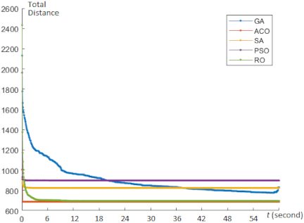
Fig. 20. Convergence behavior for the VRP optimization.
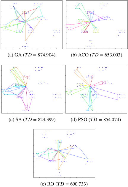
Fig. 21. Visual results of VRP problem using (a) GA, (b) ACO, (c) SA, (d) PSO, and (e) RO.
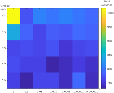
Fig. 22. Total distance showing the effect of \(\beta\) and the greedy rate for the VRP problem.
Figure 21 shows one of the visual results of the VRP problem obtained using each algorithm, indicating that the minimum \(\mathit{TD}\) focuses on visiting nodes closer to the depot boundary.
We analyzed the relationship between \(\beta\) and the greedy rate to determine their impact on the \(\mathit{TD}\) for the VRP experiment. Fig. 22 shows the \(\mathit{TD}\), indicated by color (darker blue indicates lower \(\mathit{TD}\)), from the effects of \(\beta\) and the greedy rate. We used the average \(\mathit{TD}\) values from ten experiments, each conducted with 10000 iterations.
As shown in Fig. 22, the minimum \(\mathit{TD}\) (indicated by dark blue color) occurs at a high greedy rate (0.7 and 0.9) with low \(\beta\). For this VRP problem, more experiments are needed to generalize the effects of \(\beta\) and the greedy rate on reducing the \(\mathit{TD}\) owing to the constraints of the number of vehicles and vehicle capacity. However, from the experiment shown in Fig. 22, better performance with minimum \(\mathit{TD}\) may commonly be achieved by a higher greedy rate combined with a lower \(\beta\).
Among all the experimental schemes for the centroid optimization problem, the proposed RO algorithm achieved the best performance. This means that RO can provide the best solution, in terms of both accuracy and speed, to solve continuous optimization problems such as centroid optimization. In the case of TSP and VRP, RO is also applicable to combinatorial optimization problems, such as TSP and VRP, but it still struggles to compete with ACO, which is the most effective method for these problems. Overall, across all experiments, our proposed RO algorithm can be considered as an alternative solution for both continuous and combinatorial optimization problems, providing a better trade-off between accuracy and execution time.
5. Conclusion
We introduce a novel optimization algorithm called reinforced optimization (RO) that adapts the principles from RL to address objective-based problems. This algorithm incorporates two core concepts from RL: (1) reward and penalty and (2) exploration versus exploitation. It models the problem states as sequences of rewards and updates these states based on the direction of each step. Each action taken to update the state is evaluated according to a defined objective. To assess the effectiveness of the proposed algorithm, we conducted a series of experiments on several objective-based problems: centroid optimization, TSP, and VRP. The performance of RO was compared with that of well-known optimization algorithms: GA, ACO, SA, and PSO.
Experiments on the centroid optimization problem involved various benchmark datasets: Iris, Ionosphere, Wine, and Heart. From experiments with four datasets, the proposed RO algorithm achieved a minimum SSE: 78.942 (Iris), 2419.365 (Ionosphere), 2396153.422 (Wine), and 364425.032 (Heart), compared with other algorithms, GA, ACO, and SA. RO also achieved SSE values close to those of PSO with faster computational time: 940 ms vs. 19680 ms for Iris; 4720 ms vs. 12100 ms for Ionosphere; 3200 ms vs. 16540 ms for Wine; and 2360 ms vs. 17120 ms for Heart. From these experiments, the proposed RO algorithm achieves a better trade-off between accuracy and computational time for the centroid optimization problem. For the experiment of the TSP, the proposed RO algorithm achieved a total distance of 83.958, compared with GA, SA, and PSO, which reached 191.947, 87.564, and 434.674, respectively. For the VRP, the RO algorithm also achieved a minimum total distance of 695.445, compared with GA, SA, and PSO, which reached 830.235, 823.774, and 897.360, respectively. However, the RO algorithm was difficult to achieve a smaller total distance than ACO, which is well suited for combinatorial problems, such as the TSP and VRP. For the parameter setting of the learning rate \(\mu\), smaller values of \(\mu\) result in lower SSE values in the case of centroid optimization for all datasets (Iris, Ionosphere, Wine, and Heart); however, this requires more computational time. For the parameter settings of the learning rate \(\beta\) and the greedy rate, in the case of centroid optimization, TSP and VRP, better performance of optimization is achieved with a greedy rate and a lower \(\beta\). Across all experiments, the proposed RO algorithm can be considered as an alternative solution for both continuous and combinatorial optimization problems, providing a better trade-off between accuracy and execution time.
- [1] B. Bakker and J. Schmidhuber, “Hierarchical reinforcement learning based on subgoal discovery and subpolicy specialization,” Proc. of the 8th Conf. on Intelligent Autonomous Systems, pp. 438-445, 2004.
- [2] K. Matsuda et al., “Hierarchical reward model of deep reinforcement learning for enhancing cooperative behavior in automated driving,” J. Adv. Comput. Intell. Intell. Inform., Vol.28, No.2, pp. 431-443, 2024. https://doi.org/10.20965/jaciii.2024.p0431
- [3] M. Tan, “Multi-agent reinforcement learning: Independent versus cooperative agents,” Proc. of the 10th Int. Conf. on Machine Learning, pp. 330-337, 1993.
- [4] K. Miyazaki and K. Takadama, “Special issue on cutting edge of reinforcement learning and its hybrid methods,” J. Adv. Comput. Intell. Intell. Inform., Vol.28, No.2, p. 379, 2024. https://doi.org/10.20965/jaciii.2024.p0379
- [5] R. S. Sutton and A. G. Barto, “Reinforcement learning: An introduction,” The MIT Press, 1998.
- [6] C. I. Mary and S. V. K. Raja, “Refinement of clusters from k-means with ant colony optimization,” J. of Theoretical and Applied Information Technology, Vol.10, No.1, pp. 28-32, 2009.
- [7] C. J. Watkins and P. Dayan, “Reinforcement learning,” Encyclopedia of Cognitive Science, Nature Publishing Group, 2003.
- [8] A. Gosavi, “A reinforcement learning algorithm based on policy iteration for average reward: Empirical results with yield management and convergence analysis,” Machine Learning, Vol.55, No.1, pp. 5-29, 2004. https://doi.org/10.1023/B:MACH.0000019802.64038.6c
- [9] L. P. Kaelbling, M. L. Littman, and A. W. Moore, “Reinforcement learning: A survey,” J. of Artificial Intelligence Research, Vol.4, No.1, pp. 237-285, 1996. https://doi.org/10.1613/jair.301
- [10] R. A. C. Bianchi, R. Ros, and R. L. de Mantaras, “Improving reinforcement learning by using case based heuristics,” Proc. of the 8th Int. Conf. on Case-Based Reasoning, pp. 75-89, 2009. https://doi.org/10.1007/978-3-642-02998-1_7
- [11] C. Szepesvári, “Algorithms for reinforcement learning,” Springer, 2010. https://doi.org/10.1007/978-3-031-01551-9
- [12] D. Kitakoshi, H. Shioya, and M. Kurihara, “Analysis of a method improving reinforcement learning agents’ policies,” J. Adv. Comput. Intell. Intell. Inform., Vol.7, No.3, pp. 276-282, 2003. https://doi.org/10.20965/jaciii.2003.p0276
- [13] J. Strahl, T. Honkela, and P. Wagner, “A Gaussian process reinforcement learning algorithm with adaptability and minimal tuning requirements,” Proc. of the 24th Int. Conf. on Artificial Neural Networks, pp. 371-378, 2014. https://doi.org/10.1007/978-3-319-11179-7_47
- [14] M. D. Vose, “The simple genetic algorithm: Foundations and theory,” The MIT Press, 1999. https://doi.org/10.7551/mitpress/6229.001.0001
- [15] S. Ding et al., “Improved genetic algorithm for train platform rescheduling under train arrival delays,” J. Adv. Comput. Intell. Intell. Inform., Vol.27, No.5, pp. 959-966, 2023. https://doi.org/10.20965/jaciii.2023.p0959
- [16] K. Ono and Y. Hanada, “Self-organized subpopulation based on multiple features in genetic programming on GPU,” J. Adv. Comput. Intell. Intell. Inform., Vol.25, No.2, pp. 177-186, 2021. https://doi.org/10.20965/jaciii.2021.p0177
- [17] K.-S. Hung, S.-F. Su, and Z.-J. Lee, “Improving ant colony optimization algorithms for solving traveling salesman problems,” J. Adv. Comput. Intell. Intell. Inform., Vol.11, No.4, pp. 433-442, 2007. https://doi.org/10.20965/jaciii.2007.p0433
- [18] M. Dorigo and T. Stützle, “Ant colony optimization,” Bradford Books, 2004.
- [19] C. Ratanavilisagul, “Modified ant colony optimization with route elimination and pheromone reset for multiple pickup and multiple delivery vehicle routing problem with time window,” J. Adv. Comput. Intell. Intell. Inform., Vol.26, No.6, pp. 959-964, 2022. https://doi.org/10.20965/jaciii.2022.p0959
- [20] J. Zheng and X. Gan, “A hybrid algorithm based on multi-agent and simulated annealing,” Proc. of the 2011 Int. Conf. on Future Wireless Networks and Information Systems, Vol.1, pp. 343-351, 2012. https://doi.org/10.1007/978-3-642-27323-0_44
- [21] J. Liu, X. Gao, and X. Chen, “Feasibility analysis of optimization models for natural gas distribution networks using machine learning,” J. Adv. Comput. Intell. Intell. Inform., Vol.29, No.3, pp. 614-622, 2025. https://doi.org/10.20965/jaciii.2025.p0614
- [22] H. Takano, J. Murata, Y. Maki, and M. Yasuda, “Improving the search ability of tabu search in the distribution network reconfiguration problem,” J. Adv. Comput. Intell. Intell. Inform., Vol.17, No.5, pp. 681-689, 2013. https://doi.org/10.20965/jaciii.2013.p0681
- [23] I. C. Trelea, “The particle swarm optimization algorithm: Convergence analysis and parameter selection,” Information Processing Letters, Vol.85, No.6, pp. 317-325, 2003. https://doi.org/10.1016/S0020-0190(02)00447-7
- [24] W. S. Chai, M. I. F. bin Romli, S. B. Yaakob, L. H. Fang, and M. Z. Aihsan, “Regenerative braking optimization using particle swarm algorithm for electric vehicle,” J. Adv. Comput. Intell. Intell. Inform., Vol.26, No.6, pp. 1022-1030, 2022. https://doi.org/10.20965/jaciii.2022.p1022
- [25] T. Matsui et al., “Particle swarm optimization for jump height maximization of a serial link robot,” J. Adv. Comput. Intell. Intell. Inform., Vol.11, No.8, pp. 956-963, 2007. https://doi.org/10.20965/jaciii.2007.p0956
- [26] M. Alzakan et al., “Enhancing k-means clustering results with gradient boosting: A post-processing approach,” Int. J. of Advanced Computer Science and Applications, Vol.15, No.2, pp. 913-921, 2024. https://doi.org/10.14569/IJACSA.2024.0150292
- [27] Y. M. Cheung, “ mathrm{k}^{*} k*-Means: A new generalized k k-means clustering algorithm,” Pattern Recognition Letters, Vol.24, No.15, pp. 2883-2893, 2003. https://doi.org/10.1016/S0167-8655(03)00146-6
- [28] S. S. Khan and A. Ahmad, “Cluster center initialization algorithm for K K-means clustering,” Pattern Recognition Letters, Vol.25, No.11, pp. 1293-1302, 2004. https://doi.org/10.1016/j.patrec.2004.04.007
- [29] A. R. Barakbah and Y. Kiyoki, “A pillar algorithm for K-means optimization by distance maximization for initial centroid designation,” 2009 IEEE Symp. on Computational Intelligence and Data Mining, pp. 61-68, 2009. https://doi.org/10.1109/CIDM.2009.4938630
- [30] R. Matai, S. Singh, and M. L. Mittal, “Traveling salesman problem: An overview of applications, formulations, and solution approaches,” D. Davendra (Ed.), “Traveling Salesman Problem, Theory and Applications,” pp. 1-24, IntechOpen, 2010. https://doi.org/10.5772/12909
- [31] D. S. Johnson, “Local optimization and the traveling salesman problem,” Proc. of the 17th Int. Colloquium on Automata, Languages and Programming, pp. 446-461, 1990. https://doi.org/10.1007/BFb0032050
- [32] C. Chang, J. Cao, N. Weng, and G. Lv, “Ant colony optimization parameters control based on evolutionary strength,” IEEE 31st Int. Conf. on Tools with Artificial Intelligence, pp. 448-455, 2019. https://doi.org/10.1109/ICTAI.2019.00069
- [33] M. Clauß, M. Bernt, and M. Middendorf, “A common interval guided ACO algorithm for permutation problems,” 2013 IEEE Symp. on Swarm Intelligence, pp. 64-71, 2013. https://doi.org/10.1109/SIS.2013.6615160
- [34] G. Laporte, “The vehicle routing problem: An overview of exact and approximate algorithms,” European J. of Operational Research, Vol.59, No.3, pp. 345-358, 1992. https://doi.org/10.1016/0377-2217(92)90192-C
This article is published under a Creative Commons Attribution-NoDerivatives 4.0 Internationa License.