
Paper:
Modeling of Higher-Order Rotor Flap Angle Dynamics for Flybarless Uncrewed Helicopters in High-Speed Flight
Hiroaki Nakanishi
 and Yoshiki Nishimoto
Kyoto University
Kyotodaigaku-Katsura, Nishikyo-ku, Kyoto 615-8540, Japan

Stable autonomous flight at high speeds is essential to expand the operational capabilities of flybarless uncrewed helicopters. This study develops a high-fidelity flapping dynamics model to accurately describe rotor behavior at high speeds. We derive a dynamics model that incorporates higher-order terms of the advance ratio. By expanding the flapping angle into a Fourier series, we obtain an n-th-order constant-coefficient differential equation model that accounts for inter-harmonic coupling. Numerical simulations were conducted at low (μx=0.04) and high (μx=0.25) speeds. Power spectral density analysis revealed that higher-order harmonics (2 /rev and 3 /rev) become significant at high speeds, rendering the conventional first-order approximation inadequate. Furthermore, the impact on the aerodynamic forces and moments of the rotor was quantified. In high-speed flight, the first-order model produces substantial errors in lateral force, drag, and moments owing to lift asymmetry between blades. Second-order or higher models significantly improve accuracy. Considering the balance between computational load and precision, a second-order model is the most practical choice for high-speed aerodynamic evaluation. These findings provide fundamental insights for the advanced control system design of high-speed flybarless uncrewed helicopters.
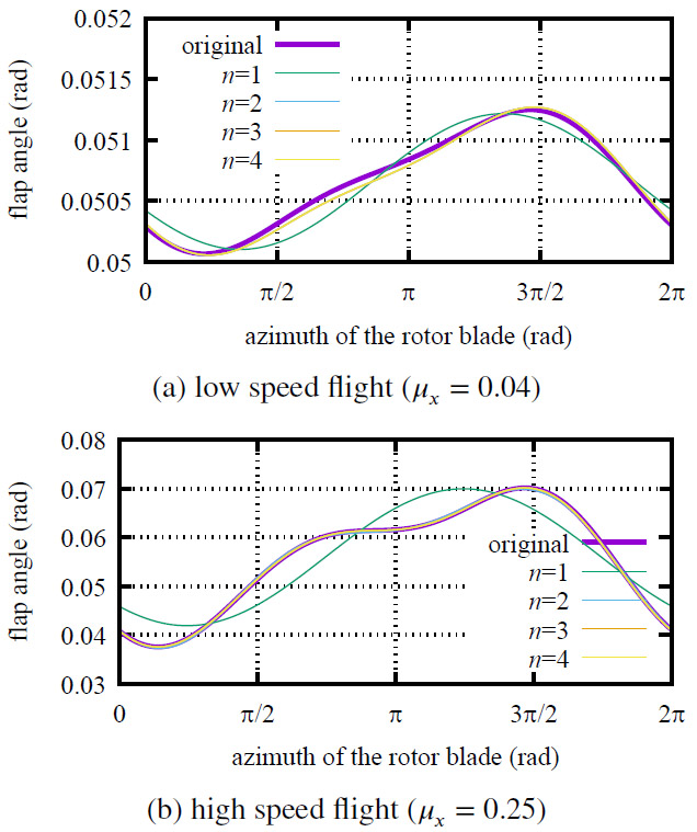
Flap angle models at low and high speed. n is the harmonic expansion order
1. Introduction
In addition to agricultural applications and disaster response 1, the use of uncrewed helicopters is expected to expand into logistics and transportation. To extend the operational envelope, establishing stable autonomous flight control in high-speed regimes is indispensable. A flight dynamics model capable of precisely describing rotor behavior is essential for high-speed flight.
Modeling of the flap angle, a critical factor determining the direction of rotor aerodynamic forces, has been extensively studied through flight-data calibration 2, models for small-scale helicopters 3, and improved induced-velocity distributions 4. However, these studies are primarily limited to low-speed flight conditions. Even in studies addressing forward flight 5,6, higher-order terms of the advance ratio \(\mu\) are generally neglected, rendering them insufficient for describing the dynamics in the high-speed regimes targeted in this study. Furthermore, models compatible with high-speed flight 7 frequently include azimuth-dependent time-varying terms, which pose significant challenges for control system design and real-time computation.
This study focuses on flybarless helicopters, which lack mechanical flybars. Although flybarless configurations are lighter and more energy-efficient, they exhibit large cross-axis coupling and small time constants relative to disturbances 4. For such inherently unstable aircraft, a concise yet high-fidelity dynamics model is indispensable for autonomous high-speed flight.
The purpose of this study is to construct a model that accurately represents the flap angle response of flybarless helicopters during high-speed flight and to clarify the aerodynamic differences from low-speed flight. In high-speed regimes, the inflow owing to forward motion becomes dominant, and the effects of higher-order terms of the advance ratio cannot be ignored. This paper proposes a flap angle dynamics model that incorporates these high-speed effects. The analysis employs the Floquet theory 8 to demonstrate changes in the response period, and numerical simulations confirm the occurrence of higher-order harmonic oscillations. Furthermore, by expanding the flap angle in a Fourier series, we derive a constant-coefficient model that eliminates the rotor blade’s azimuth angle \(\psi\) and verify its validity. Finally, we demonstrate that accounting for higher-order harmonic components is critical for accurately calculating rotor forces and moments in high-speed flight.
The remainder of this paper is structured as follows: Section 2 reviews the basic models, and Section 3 describes the derivation and analysis of the high-speed flight model. Section 4 verifies the effectiveness of higher-order harmonic terms. Finally, Section 5 presents the conclusions.
2. Model of Flap Angle Dynamics
2.1. Coordinate Systems
The coordinate systems shown in Figs. 1 and 2 are defined. First, we define the hub coordinate system \(F_h\), which is fixed to the fuselage and centered at the rotor hub. Each axis of \(F_h\) is parallel to the fuselage axes, with the positive \(x_h\)-axis pointing toward the nose, the positive \(y_h\)-axis pointing to starboard, and the positive \(z_h\)-axis pointing downward relative to the fuselage.
Subsequently, we define the blade coordinate system \(F_b\), which rotates with the blades. For the sake of simplifying the analysis, the flapping hinge is assumed to be at the same location as the rotor hub, with no hinge offset. The \(x_b\)-axis of \(F_b\) is in the spanwise direction of the blade (positive toward the tip), the \(y_b\)-axis is in the chordwise direction (positive in the direction of rotation), and the \(z_b\)-axis is chosen to form a right-handed system.
The main rotor is assumed to rotate at a constant angular velocity \(\Omega\) clockwise as viewed from above, and the azimuth angle \(\psi = \Omega t\) is defined with the nose direction as the reference. Additionally, the flap angle \(\beta\) is defined as the angle formed by the \(x_b\)-axis of the rotor blade with the \(x_h\)-\(y_h\) plane, with the upward (coning) direction taken as positive.
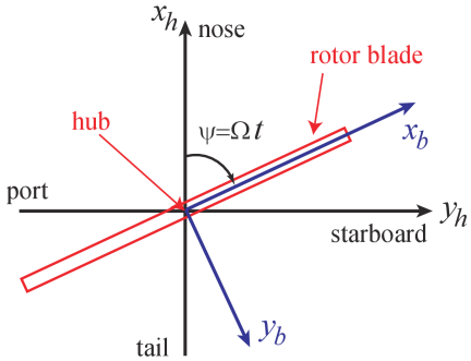
Fig. 1. Coordinate systems \(F_h\), \(F_b\) and blade azimuth angle \(\psi\).
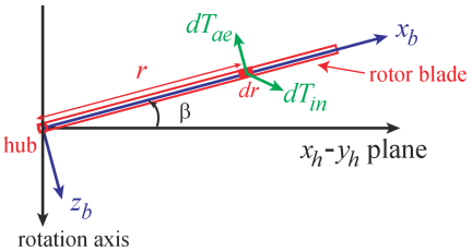
Fig. 2. \(F_b\) coordinate axis and blade flap angle \(\beta\) and forces acting on the blade element.
2.2. Equation of Motion for Flap Angle
The equation of motion for the flap angle of the rotor blade is derived from the balance of moments about the flapping hinge. Considering a minute blade element \(dr\) located at a distance \(r\) from the hub, we define the inertial force acting on it as \(dT_{in}\) and the aerodynamic force be \(dT_{ae}\) as shown in Fig. 2. The moment balance is expressed by the following equation:
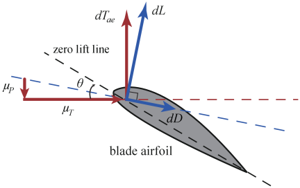
Fig. 3. The flow velocity and aerodynamic forces acting on the blade element.
Next, the aerodynamic force \(dT_{ae}\) acting on the element is determined. For the velocity components of the element shown in Fig. 3, the rotor rotation axis parallel component \(\mu_P\) and the perpendicular component \(\mu_T\), non-dimensionalized by the tip speed \(R\Omega\), are as follows:
Based on blade element theory, using the lift curve slope \(a\) and the chord length \(c\), \(dT_{ae}\) is approximated by the following equation:
2.3. Inflow Ratio Model
Under the high-speed flight conditions targeted in this study, it is essential to appropriately evaluate the air inflow condition (inflow ratio) to the rotor disk plane. Assuming steady level forward flight (\(\mu_y = 0, \mu_z = 0\)), Fig. 4 shows the relationship between the inclination angle \(i\) of the tip path plane (TPP) and the airspeed. Under this assumption, the non-dimensionalized airspeed \(\mu_\infty\) of the helicopter is simply equal to the forward speed component:
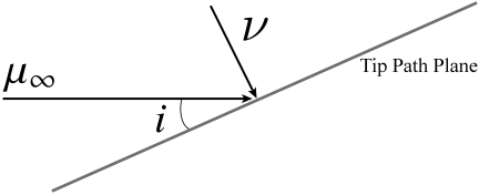
Fig. 4. The inclination of tip path plane.
The advance ratio \(\mu\) and the inflow ratio \(\lambda\) are defined by the following equations as a superposition of the inflow component due to the airspeed of the helicopter and the induced velocity \(\nu\) associated with the rotation of the rotor.
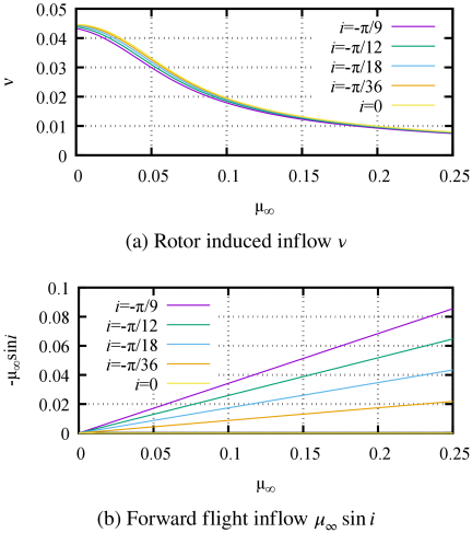
Fig. 5. Comparison of each term in the inflow ratio against forward flight velocity.
In contrast, regarding the high-speed flight that is the main focus of this study, we assume that \(\mu_y\) is small, while \(\mu_\infty \sin i\) becomes non-negligible relative to \(\nu\). As shown in Figs. 5(a) and (b), with the increase in flight speed, the influence of the induced velocity \(\nu\) relatively decreases, and instead, the influence of the inflow component \(\mu_\infty \sin i\) due to the forward tilt of the fuselage becomes dominant. Therefore, as a model for the inflow ratio in the high-speed regime, a format that accounts for all terms is used, as shown in the following equation:
3. Changes in Flapping Angle Characteristics Due to Flight Speed
3.1. Targeted Helicopter and Rotor Parameters
This study targets the uncrewed helicopter “Fazer” with the flybar removed 4.
Its primary parameters are listed in Table 1. In this paper, all physical parameters and specifications are standardized to SI units, and angles are measured in radians.
| Parameter | Symbol | Value |
| Air density | \(\rho\) | 1.225 |
| Acceleration of gravity | \(g\) | 9.8 |
| Main rotor angular velocity | \(\Omega\) | 89 |
| Rotor blade radius | \(R\) | 1.56 |
| Gross mass | \(m\) | 82.3 |
| Blade moment of inertia | \(I_\beta\) | 1.021 |
| Blade mass per unit length | \(m_b\) | 0.807 |
| Flapping stiffness | \(k_\beta\) | 1627 |
| Lock number | \(\gamma\) | 3.3433 |
| Lift curve slope | \(a\) | 1.57 |
| Chord length | \(c\) | 0.3 |
| Moment of inertia about \(X\)-axis | \(I_{xx}\) | 1.6 |
| Moment of inertia about \(Y\)-axis | \(I_{yy}\) | 10.9 |
| Moment of inertia about \(Z\)-axis | \(I_{zz}\) | 10.2 |
| \(X\)-distance from CG to tail rotor | \(l_{tr}\) | 2.5 |
| \(Z\)-distance from CG to tail rotor | \(h_{tr}\) | 0.3 |
| \(Z\)-distance from CG to hub | \(h_h\) | 0.42 |
3.2. Steady Forward Flight Conditions and Equation of Motion
This section examines how flight speed influences the characteristics of the flap angle \(\beta\). Note that the general governing equations prior to any simplification are provided in Appendix A. To simplify the discussion and derive the specific equation of motion for steady forward flight (Eq. (13)), we make the following assumptions:
-
・
The flight speed is constant, and the helicopter is flying forward. That is, \(\mu_x \neq 0\) and \(\mu_y = \mu_z = 0\).
-
・
The attitude of the helicopter is kept constant. That is, \(p = q = r = 0\).
-
・
\(\theta_0\), \(\theta_{1c}\), and \(\theta_{1s}\) are constant.
-
・
The blade parameters \(m_r, \beta, \theta, a, c\) are constant regardless of the spanwise position.
Under these assumptions, the equation of motion for the rotor flap angle is as follows:
The coefficients of \(\beta\) and \(\dot{\beta}\) on the left-hand side of Eq. (13) are functions of \(\psi\). This indicates that the equation of motion for the rotor flap angle constitutes a periodic system with time-varying coefficients. According to Floquet’s theory, the response of a periodic system subjected to periodic external forces (such as cyclic pitch control) contains not only the periodic components of the input but also higher-order harmonic components that are integer multiples of the input period. Especially under high-speed flight conditions where the contribution of higher-order components becomes significant, an approximation that limits the Fourier series expansion of \(\beta\) to only the zeroth and first orders, as in the following equation, is inadequate:
On the other hand, consider the case where flight speed is low, and the higher-order terms of \(\mu_x\), as well as the higher-order terms of the products of \(\mu_x\) with \(\theta\), \(\beta\), and their time derivatives, are sufficiently small. In this case, the equation of motion for the flap angle can be approximated as a constant-coefficient differential equation as follows:
The benchmark trim parameters and control inputs shown in Table 2 are uniquely determined from the steady-state flight equilibrium of the entire helicopter. Specifically, the trim state was calculated by constraining the vehicle velocities to the command values and the angular velocities to zero. The remaining unknown variables, including control inputs and attitude angles, were obtained by simultaneously and numerically solving the equations of motion (for the flap angle, vehicle translation, and vehicle rotation) based on the Fourier series expansion equations shown in Appendix A. This numerical solution was obtained using the “fsolve” command in Maple, which performs iterative calculations. To ensure a fair comparison of how the expansion order \(n\) affects flapping accuracy and aerodynamic calculations, this trim routine is executed using the conventional first-order flapping model (\(n = 1\)), incorporating fuselage aerodynamic drag. Once these benchmark control inputs (\(\theta_0, \theta_{1c}, \theta_{1s}\)) and attitude parameters are determined, they are kept completely constant across all simulations. For each target speed (\(\mu_x = 0.04\) and \(\mu_x = 0.25\)), we then evaluate the multi-harmonic flapping dynamics (Eq. (17)) for each order \(n\) under the exact same control benchmark. This isolated evaluation protocol allows us to evaluate the pure sensitivity of the aerodynamic force/moment estimations to the model order \(n\) under a consistent physical flight state.
| Symbol | Low-speed | High-speed |
| \(\mu_x\) | 0.04 | 0.25 |
| \(i\) | \(-5.24 \times 10^{-4}\) | \(-1.75 \times 10^{-2}\) |
| \(\theta_0\) | \(1.97\times 10^{-1}\) | \(1.51\times 10^{-1}\) |
| \(\theta_{1c}\) | \(3.16\times 10^{-2}\) | \(2.14\times 10^{-1}\) |
| \(\theta_{1s}\) | \(-1.66 \times 10^{-2}\) | \(-1.06 \times 10^{-1}\) |
3.3. Comparison of Numerical Calculation Results
Numerical solutions to the equation of motion (Eq. (13)) for the flap angle \(\beta\) under steady forward flight conditions are presented herein. We evaluate the steady-state response of \(\beta\) at both low-speed (\(\mu_x = 0.04\)) and high-speed (\(\mu_x = 0.25\)) conditions. Fig. 6 illustrates the variations in \(\beta\) as a function of the azimuth angle \(\psi\). Fig. 6 indicates that in low-speed flight, the periodic variation is dominated by the first-order component, with negligible higher-order harmonic content. These results validate the first-order expansion in Eq. (15) for low flight speeds. In contrast, in high-speed flight, \(\beta\) possesses harmonic components with respect to \(\psi\).
Figure 7 presents the power spectral density (PSD) of the flapping angle \(\beta\). Given the rotor angular velocity \(\Omega = 89\) rad/s, the fundamental rotor rotation frequency (1 /rev) corresponds to 14.2 Hz. In the figure, vertical dashed lines indicate the 1 /rev, 2 /rev, and 3 /rev frequencies for reference purposes. We find that in the low-speed regime (\(\mu_x = 0.04\)), the PSD exhibits spectral peaks only at the DC and 1 /rev frequencies. This result validates the treatment of Eq. (16) as a constant-coefficient differential equation and confirms the adequacy of the first-order expansion in Eq. (15) for low-speed conditions. In contrast, for the high-speed regime (\(\mu_x = 0.25\)), significant peaks emerge at the 2 /rev and 3 /rev frequencies in addition to the DC and 1 /rev components. These spectral characteristics demonstrate that as the advance ratio \(\mu_x\) increases, the influence of the azimuth-dependent periodic coefficients in Eq. (13) becomes non-negligible. This quantitatively proves that conventional first-order approximation models are insufficient for capturing rotor dynamics in high-speed flight regimes.
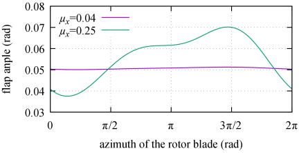
Fig. 6. Flapping angle distribution under steady forward flight conditions.
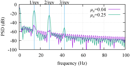
Fig. 7. Power spectral densities of flapping angle responses at different advance ratios.
4. Higher-Order Harmonic Series Expansion of Flap Angle and its Effects
4.1. Higher-Order Harmonic Series Expansion of Flap Angle
To accurately capture the flap dynamics described by Eq. (13), we expand the flap angle \(\beta\) into a higher-order harmonic series. Letting \(n\) denote the highest order of the harmonic terms considered, the expansion is given by
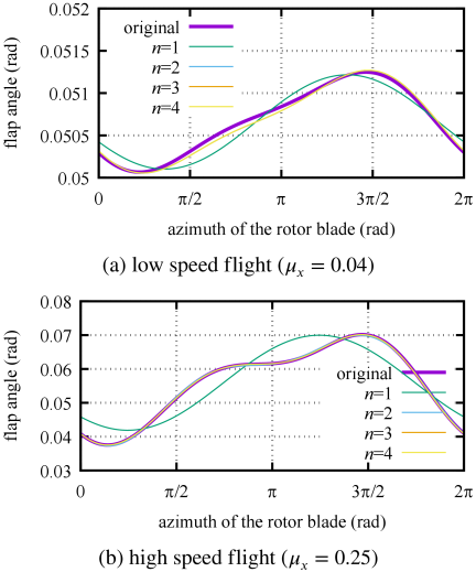
Fig. 8. Comparison of flap angle models.
We verify the modeling fidelity of the \(n\)-th order model by comparing its solution \(\beta_n(\psi)\) with the true value \(\beta(\psi)\) obtained through direct numerical integration of Eq. (13). Fig. 8 compares the flap angle responses for both low-speed and high-speed flight conditions. Additionally, we employ the mean absolute error defined by Eq. (18) as a quantitative index:
In contrast, under the high-speed flight condition (\(\mu_x = 0.25\)), expanding from a first-order to a higher-order model yields a substantial improvement in fidelity. Although accuracy further increases from \(n=2\) to \(n=3\), no significant gain is observed beyond the third-order. These results demonstrate that the conventional first-order approximation is inadequate for capturing the response characteristics in high-speed regimes. We conclude that achieving sufficient fidelity requires at least a second-order model, with a third-order or higher expansion being ideal for high-speed flight analysis.
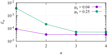
Fig. 9. Mean absolute error \(E_n\) as a function of the harmonic expansion order \(n\).
4.2. Computational Implementation and Engineering Applications
The multi-harmonic constant-coefficient formulation presented in Appendix A offers two major computational advantages depending on the intended simulation or control scenario.
Steady-State Algebraic Solution:
For steady forward flight (where transient dynamics have decayed), the time-derivatives of the Fourier coefficients can be set to zero (\(\ddot{(\cdot)} = 0\), \(\dot{(\cdot)} = 0\)). This simplifies the differential equations in Appendix A to a set of static linear algebraic equations in the form of a matrix equation:
Transient State-Space Simulation:
When transient responses are needed, the constant-coefficient system can be easily converted into a standard linear time-invariant (LTI) state-space model. Unlike Eq. (13), which requires an extremely fine integration step size to resolve the high-frequency azimuth angle \(\psi = \Omega t\), this LTI model can be simulated using a significantly larger time step (e.g., \(10\) ms), matching the update rate of standard flight control computers.
Expected practical applications of this reduced-cost, high-fidelity model include:
-
・
Application of modern flight control (e.g., inverse dynamics transformation): Advanced control frameworks are based on state-space representations. Our constant-coefficient model provides this format directly, enabling high-speed control that accounts for higher-order flapping coupling and lateral-longitudinal cross-coupling without the use of computationally intensive time-varying models.
-
・
Real-time hardware-in-the-loop (HIL) simulation: In HIL systems running on embedded flight controllers, rotor flap dynamics can be executed at standard control update rates (100–400 Hz) rather than at kilohertz update rates.
-
・
Online rotor load/vibration monitoring: Estimation of dynamic blade loads and high-order fatigue stress (2 /rev and 3 /rev components) on board during flight, which can be linked to active vibration control, such as higher harmonic control.
4.3. Impact on Evaluation of Rotor Aerodynamic Characteristics
We express the aerodynamic force components acting on the rotor in the hub coordinate system (\(x_h, y_h, z_h\))—namely thrust \(T\), lateral force \(Y\), and drag \(H\)—as follows:
To evaluate the pure sensitivity of the aerodynamic force and moment estimations to the model order \(n\), we conduct the calculations using the identical benchmark trim parameters (vehicle attitude and control inputs) fixed in Section 3.2. We take the aerodynamic characteristics obtained by directly integrating the time-varying Eq. (13) as the reference values (true values) for comparison with those obtained from the constant-coefficient \(n\)-th order models. Based on the findings in the previous section, we limit the comparison to models of order up to the third order, as no significant improvement is expected for \(n > 3\). Fig. 10 presents the normalized estimation accuracy for aerodynamic forces and moments under the high-speed flight condition of \(\mu_x = 0.25\).
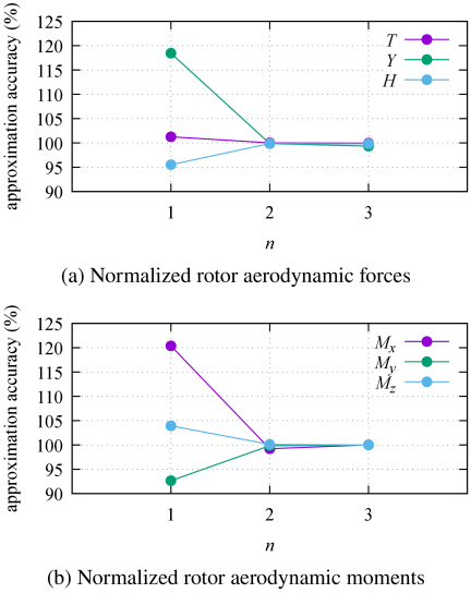
Fig. 10. Accuracy of rotor aerodynamic force and moment estimations relative to the order of harmonic expansion.
As shown in Fig. 10(a), the estimation accuracy of the aerodynamic forces significantly deteriorates with the first-order model, with substantial errors particularly in the lateral force \(Y\) and drag \(H\). This occurs because the asymmetry of the lift distribution between the advancing and retreating sides intensifies at higher forward speeds. Thus, the resulting higher-order flap angle components contribute significantly to the aerodynamic force balance. Since the first-order model neglects these components, it fails to represent this physical phenomenon. In contrast, the second- and third-order models show good agreement with the true values. It should be noted that while the normalized value for the lateral force \(Y\) at \(n=3\) (\(99.64\%\)) appears slightly less accurate than at \(n=2\) (\(100.12\%\)), this difference of less than \(0.5\%\) is not a physical degradation due to higher-order expansion. This minute discrepancy is a numerical artifact caused by the truncation of higher-order coupling terms and the limits of numerical integration (e.g., discretization and round-off errors) in Eq. (20). From an engineering perspective, both models are considered to have fully converged to the true value. We therefore conclude that a second-order model provides sufficient accuracy for describing the helicopter’s translational motion at high speeds.
Similarly, Fig. 10(b) confirms that the first-order model is inadequate for evaluating rotor aerodynamic moments. All components (\(M_{xh}\), \(M_{yh}\), \(M_{zh}\)) exhibit large errors because the first-order model fails to capture the azimuthal variation in the flap angle distribution. Conversely, adopting a second-order or higher model significantly improves estimation accuracy, with the second- and third-order models yielding nearly identical results.
These findings demonstrate that the conventional first-order model is insufficient for evaluating rotor aerodynamic characteristics in high-speed flight, underscoring the need for a second-order or higher-harmonic expansion. Furthermore, considering the trade-off between computational cost and accuracy, we conclude that a second-order model is the most practical and reasonable choice for high-speed flight analysis.
5. Conclusion
In this study, we constructed an equation of motion for the rotor flap angle that includes higher-order velocity terms to evaluate dynamic and aerodynamic characteristics during high-speed helicopter flight accurately. Furthermore, we developed a higher-order harmonic series expansion model and verified its effectiveness through numerical analysis. The primary findings of this study are as follows.
First, we established a dynamics model in the form of constant-coefficient differential equations (the \(n\)-th order model) by expanding the flap angle \(\beta\) into harmonic terms up to the \(n\)-th order. Although this model is in a constant-coefficient format suitable for high-speed computation and control system design, unlike conventional models, it accounts for coupling effects across different orders. The proposed formulation can sufficiently capture changes in the flap angle distribution with respect to the blade azimuth angle. Next, we verified the modeling fidelity of this approach across different flight speeds through numerical simulations:
-
・
In the low-speed regime (\(\mu_x = 0.04\)), the conventional first-order approximation provides sufficient accuracy, and the improvement gained from higher-order modeling plateaus beyond the second order.
-
・
In the high-speed regime (\(\mu_x = 0.25\)), the conventional first-order model is inadequate; we demonstrated that achieving sufficient fidelity requires at least a second-order, or ideally a third-order or higher, expansion.
Additionally, we investigated the impact of higher-order flap angle components on the evaluation of rotor aerodynamic forces and moments. Our results quantitatively show that first-order models produce substantial errors during high-speed flight—particularly in lateral force \(Y\), drag \(H\), and all aerodynamic moment components—because they neglect the asymmetry of lift distribution and the resulting higher-order flapping. Although using a higher-order model significantly improves evaluation accuracy, a second-order model is the most practical and reasonable choice for aerodynamic evaluation in high-speed regimes, considering the trade-off between computational cost and modeling fidelity.
In summary, this study demonstrates that adopting a higher-order harmonic expansion is essential for appropriately evaluating rotor behavior and aerodynamic characteristics at high speeds. The obtained results provide fundamental insights into the motion analysis of future high-speed helicopters and the design of high-performance control systems. Future work will involve evaluating flap angle motion in non-equilibrium states, integrating the proposed formulation with higher-order dynamic inflow models such as the Peters–He model 10,11, and validating the combined framework against actual flight data.
Acknowledgments
This work was supported by JSPS KAKENHI Grant Number 24K07418.
- [1] A. Sato and H. Nakanishi, “Observation and Measurement in Disaster Areas Using Industrial Use Unmanned Helicopters,” 2014 IEEE Int. Symp. on Safety, Security, and Rescue Robotics, 2014. https://doi.org/10.1109/SSRR.2014.7017671
- [2] K. Hui and R. Srinivasan, “The Inclusion of Higher-Order Rotor Dynamics to Improve the Dynamic Model of a Single-Rotor Helicopter in Hover,” NATO Symp. on System Identification for Integrated Aircraft Development and Flight Testing, 2009.
- [3] S. Bhandari and R. Colgren, “High-Order Dynamics Models of a Small UAV Helicopter Using Analytical and Parameter Identification Techniques,” J. of the American Helicopter Society, Vol.60, No.2, pp. 1-10, 2015. https://doi.org/10.4050/JAHS.60.022012
- [4] A. Sato, H. Nakanishi, and H. Okawa, “Stabilizer-bar’s Effect on Flight Dynamics of Unmanned Helicopter,” J. of the Japan Society for Aeronautical and Space Sciences, Vol.63, Issue 2, pp. 68-76, 2015. https://doi.org/10.2322/jjsass.63.68
- [5] B. Zhu and Z. Zuo, “Approximate analysis for main rotor flapping dynamics of a model-scaled helicopter with Bell-Hiller stabilizing bar in hovering and vertical flights,” Nonlinear Dynamics, Vol.85, No.3, pp. 1705-1717, 2016. https://doi.org/10.1007/s11071-016-2788-z
- [6] M. Alexander, “Identification of Higher-Order Rotor Flapping Dynamics Model Structures Using Explicit Soft Inplane Hingeless Rotor Hub State Measurements of the NRC Bell 412 Advanced System Research Aircraft,” Proc. of the Vertical Flight Society 80th Annual Forum and Technology Display, 2024. https://doi.org/10.4050/F-0080-2024-1396
- [7] J. R. Majhi and R. Ganguli, “Helicopter blade flapping with and without small angle assumption in the presence of dynamic stall,” Applied Mathematical Modeling, Vol.34, Issue 12, pp. 3726-3740, 2010. https://doi.org/10.1016/j.apm.2010.02.010
- [8] W. Johnson, “Helicopter Theory,” Courier Corporation, 2012.
- [9] W. Johnson, “Rotorcraft Aeromechanics,” Cambridge University Press, 2013. https://doi.org/10.1017/CBO9781139235655
- [10] D. A. Peters, D. D. Boyd, and C. J. He, “Finite-State Induced-Flow Model for Rotors in Hover and Forward Flight,” J. of the American Helicopter Society, Vol.34, No.4, pp. 5-17, 1989. https://doi.org/10.4050/JAHS.34.5
- [11] D. A. Peters and C. J. He, “Finite state induced flow models. II – Three-dimensional rotor disk,” J. of Aircraft, Vol.32, No.2, pp. 323-333, 1995. https://doi.org/10.2514/3.46719
Appendix
Appendix A. Fourth-Order Model
This appendix presents the explicit governing equations for the fourth-order harmonic expansion model. These equations represent the general formulation prior to the simplifications introduced in Section 3.2. Specifically, the equation of motion analyzed in the main text (Eq. (13)) is a special case derived from this general model by applying the steady forward flight assumptions (e.g., setting terms such as \(p\), \(q\), and \(\mu_y\) to zero). Note that models of a lower order than the fourth order (e.g., \(n=1, 2, 3\)) can be obtained by truncating the corresponding higher-order terms from this set of equations.
This article is published under a Creative Commons Attribution-NoDerivatives 4.0 Internationa License.