
Paper:
Parameter Identification of Mecanum Wheel Robot Using Descent with Stability Criterion
Shangshang Nie*, Naoki Igo**
 , and Kiyoshi Hoshino*,***,†
*Institute of Systems and Information Engineering, University of Tsukuba
1-1-1 Tennodai, Tsukuba, Ibaraki 305-8577, Japan
**Faculty of Information Design, Tokyo Information Design Professional University
2-7-1 Komatsugawa, Edogawa-ku, Tokyo 132-0034, Japan
***School of Science and Technology, Meiji University
1-1-1 Higashi-Mita, Tama-ku, Kawasaki, Kanagawa 214-8571, Japan
†Corresponding author

It is challenging to model a four-wheeled Mecanum robot with an input-signal frequency that is limited to 10 Hz by design, owing to the low-frequency input and unknown motor dynamics. To address this issue, Nakagawa et al. proposed a reduced-order exhaustive search approach, which is limited by low high-speed accuracy and long computation times. Therefore, this study represented the wheel dynamics as a discrete difference equation and estimated relevant parameters using the gradient descent method. Additionally, Routh–Hurwitz stability constraints were incorporated using Karush–Kuhn–Tucker conditions: whenever an updated solution violated stability, it was projected back into the feasible region to ensure all system poles stay in the left half-plane. The proposed method achieved an almost zero relative steady-state error of -4.41×10⁻⁸, representing an improvement of 2–5 orders of magnitude compared to those obtained using the method proposed by Nakagawa et al. (2.79×10⁻⁶) and standard gradient descent method (1.09×10⁻²). It also maintained comparable dynamic performance with a rise time of 0.12 s and a settling time of 0.23 s, aligning with the rise time (0.11 s) and settling time of the robot (0.25 s), respectively. These results indicated the effectiveness of introducing stability constraints into parameter estimation for low input signal frequency systems, ensuring both accuracy and system stability.
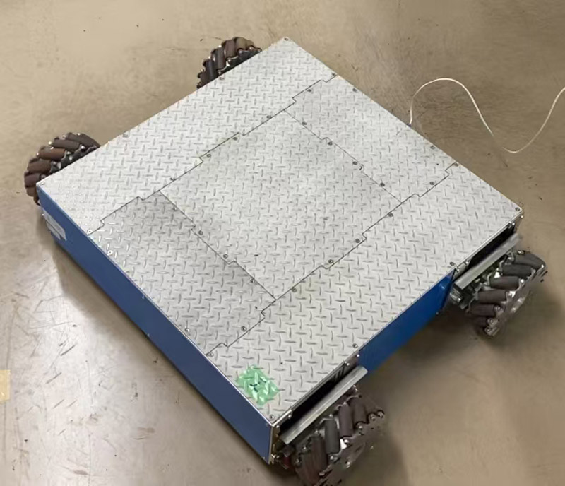
Mecanum-wheeled robot used in study
1. Introduction
Tankendo is a Japanese sport in which two participants, armed with a 53-cm bamboo sword and protective gear 1, engage in combat on a \(9\times 9\) m\(^2\) field. Traditional Tankendo training involves striking a wooden stake. Recently, robotic training has been proposed to evaluate the effectiveness of techniques (“waza” in Japanese) in the absence of opponents 2,3. To ensure the effectiveness of such training robots, an accurate kinematic model is essential for the controller design and safety certification during system testing.
For this purpose, a previous study selected a four-wheeled Mecanum robot (Tosa Denshi Company Limited) as a robotic movement platform, which was capable of forward motion, 360° rotation, and turning. However, the robot could accept control signals only at 10 Hz, and the characteristics of the motor and driver remain unknown 4. These features pose significant challenges in system identification.
Mecanum robots are widely used in various applications 5,6, and extensive research has been conducted on their modeling and control 7,8,9. However, most existing studies assume high-frequency inputs and do not address the challenges imposed by low input frequencies, as well as by the uncertain specifications of motor and driver.
To address the issue of uncertain motor and driver specifications, Nakagawa et al. 10 reduced the number of unknown parameters of a model by reducing the order of the motor model and choosing a proportional-integral controller instead of a proportional-integral-derivative (PID) controller. Subsequently, three unknown parameters were separated into two sets, and an alternating iterative procedure was employed. One group was fixed, while the other was varied to minimize the sum of the squared errors between the model and robot outputs. The roles of the groups were then reversed, and the process was repeated twice.
This method determines all possible parameter combinations by employing an exhaustive search method based on a predefined range and step size, thereby increasing the possibility of obtaining an effective solution. In addition, it separates the problem of solving three parameters into several two-dimensional or one-dimensional subproblems, thereby substantially reducing the computational complexity.
However, in the method proposed by Nakagawa et al., the value of the first fixed parameter, the range of the parameter value, and the step size of the exhaustive search must be determined by prior knowledge. Although the separation of the three-parameter estimation problem reduces the complexity of the computation, the exhaustive search method markedly increases the computational load. Finally, parameter estimation is performed using only data at 60 rpm; this may capture only the dynamic characteristics at medium speeds, while neglecting potential nonlinearities and other dynamic differences at low and high speeds. This can result in larger prediction errors under both low- and high-speed conditions.
The gradient descent method 11 is commonly used for parameter identification to reduce the computational load of the method proposed by Nakagawa et al. The parametric model identification method uses known input–output data to establish a mathematical model of the system. The gradient descent method focuses on the minimum difference between the model output and actual output as the goal and adjusts the model parameters using the gradient values obtained from each step of parameter updating to approach the goal iteratively. This method is often used to solve parameter estimation and optimization problems 12,13. However, the efficiency of this method depends on the choice of initial values, and the method has the disadvantage of easily falling into local optima. Several methods have been developed to address this issue 14,15,16. Moreover, accurate parameter estimation requires the system inputs to have a broad frequency range, including both high and low frequencies, which is not achieved in this study as the input signal frequency of the robot is limited 17.
The goal of this study is not to improve control performance under low-update frequency conditions but rather to develop a system identification method that remains feasible and effective when only low-frequency command signals are available. This study proposes a method based on the gradient descent method. System stability was used as a constraint for parameter identification. First, the system was represented by a difference equation. The parameters were then fitted by minimizing the error between the model output and the actual output obtained from experiments. The stability condition, based on the Routh–Hurwitz criterion, was introduced into this problem. This ensures that the model not only minimizes the error but also remains stable during the parameter estimation process. By contrast, conventional system-identification methods typically do not incorporate stability constraints and their model performance entirely depends on error minimization. In addition, although this method requires the computation of stability constraints at each gradient descent iteration, which leads to a decrease in computational speed compared with that of the standard gradient descent method, the proposed method is more computationally efficient overall than the method proposed by Nakagawa et al.
2. System Overview
2.1. Mecanum Robot Configuration
This study used a four-wheeled Mecanum carrier capable robot manufactured by Tosa Denshi Company Limited. A direct-current (DC) motor was used to drive the wheels of the robot. The dimensions of the robot are shown in Fig. 1. All units are in millimeters.
The body of the robot was rectangular. All four wheels were mounted parallel to one side of the robot, and the rollers on the wheels were oriented at an angle of 45° to the wheels, as shown in Fig. 1. The robot could move in all directions by adjusting the speed and direction of the wheels, which were controlled independently. The robot was capable of performing various motions, including straight-line movement, 360° rotation, and turning.
The robot received a control signal input every 0.1 s. The control signal consisted of three parts: target wheel velocity \(V\) [rpm], target velocity direction \(\theta\) [°], and target turning speed \(VC\) [rpm]. The resolutions of \(V\) and \(VC\) were 1 rpm, and that of \(\theta\) was 1° 18.
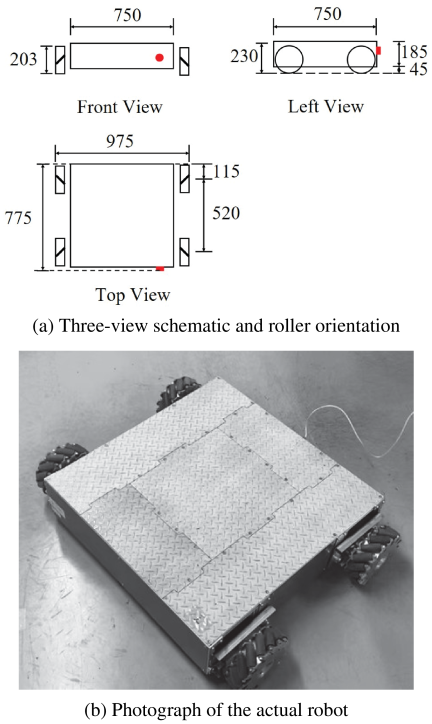
Fig. 1. Overview of the Mecanum wheel robot.
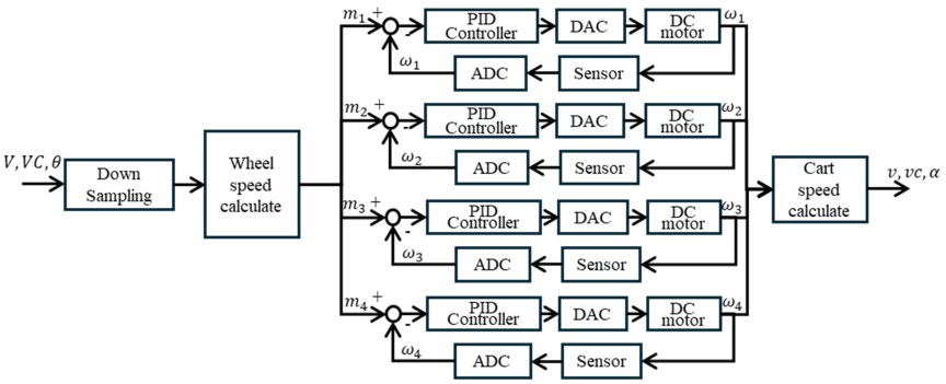
Fig. 2. Block diagram of the Mecanum wheel robot model.
2.2. Modeling of Mecanum Robot
The robot model consisted of two parts: the kinematic equation between the wheel rotational velocity and the overall motion of the robot and the relationship between the input driving signal and the wheel rotational velocity, which was represented as a difference equation.
The inputs of this model were defined as the target wheel velocity \(V\), target velocity direction \(\theta\), and target turning speed \(VC\). The outputs were defined as the actual outputs of the robot model: wheel velocity \(v\), velocity direction \(\alpha\), and turning speed \(vc\).
The system configuration of the robot is described as follows: the host computer converted the control signal into the target velocity of each wheel and sent it to the four motor drivers that drove the motors. The internal structure of this robot is shown in Fig. 2. In Fig. 2, the abbreviations DAC and ADC stand for digital-to-analog converter and analog-to-digital converter, respectively.
All wheel models were identical, with each model comprising a PID controller, DC motor, reduction gearbox, and wheel.
The command-level relationship between the velocity of the robot and target rotational velocity of each wheel is given by Eq. (1). This equation was provided in the robot manual.
3. System Identification
System identification is the process of establishing a mathematical model of a system to describe its dynamic behavior using known input and output data. This process consists of four steps: data acquisition, model selection, parameter estimation, and model validation.
3.1. Wheel Control System Modeling
Based on the analysis of the system components (Section 2), the wheel system was modeled as follows.
Equations (3) and (4) are obtained based on Kirchhoff’s current law and Ampère’s force law 21.
Substituting \(i\) in Eq. (4) into Eq. (3) yields Eq. (5), which is a differential equation for the DC motor.
The DC motors and wheels are represented by continuous values, which must be discretized for modeling. Eqs. (6) and (7) were derived using the Taylor series expansion.
Substituting Eqs. (6) and (7) into Eq. (5) yields Eq. (8), which is a discrete equation for the DC motor.
The PID controller, DC motor, and wheel, together with its reduction gearbox, were parameterized as an entire system. This is because the robot is like a black box which cannot be disassembled; therefore, it was not possible to input the motor parameters separately to obtain its response for system identification. Only the input signal was sent to the robot, and the rotation of the wheel was measured as the system output. The discrete formula for the PID controller is as follows:
To derive Eq. (11), the difference form \(\Delta u(k)=u(k)-u(k-1)\) was first derived based on Eqs. (9) and (10), which eliminated the integral term. A similar form of \(\Delta u(k)\) was also derived from Eq. (8). By equating the two expressions of \(\Delta u(k)\) and isolating \(\omega(k+1)\), a difference equation was obtained as follows:
3.2. Gradient Descent Based Parameter Estimation
Parameter estimation was conducted by measuring the rotational velocity of robot wheel \(n(k)\) and then applying the same signal into the wheel model. The model output rotational velocity was denoted as \(\omega(k)\). The average squared error between \(n(k)\) and \(\omega(k)\) at each moment was used as the objective function, and the parameters of the model were estimated to minimize the value of the objective function. That is,
However, depending on the initial value selection, the gradient descent method may potentially converge to a local optimum. Therefore, a method is required to address this issue.
The step response data for parameter estimation cannot cover all dynamic or static characteristics of the robot. Moreover, considering the numerical values of mean squared error (MSE) as the only criterion may not reflect the physical characteristics of the robot.
One way to narrow the region of feasible solutions is to add constraints into the gradient descent process. Introducing the physical or system characteristics of the robot as constraints into the gradient descent process can ensure that the model has the same physical or system characteristics as that of the robot when obtaining the parameters. As the wheel of the robot is a stable system, system stability is a satisfactory constraint for optimizing the gradient descent process.
The Routh–Hurwitz stability criterion 22, which determines system stability by the change in the sign of the coefficients in the Routh arrays, was used as a condition for the stability constraints of the system.
The Routh–Hurwitz stability criterion is only applicable to continuous systems. Therefore, a bilinear transformation was used to map the unit circle stability region of the discrete system to the left half-plane of the continuous system. The model equation was first written in the \(z\)-domain form as follows:
A bilinear transformation was then applied to \(G(z)\). Substituting equation \(z=(1+(\tau/2)\omega)/(1-(\tau/2)\omega)\) into Eq. (13) yields Eq. (14):
According to the Routh–Hurwitz stability criterion, the Routh array was obtained as follows:
Thus, \(b_3\), \(b_2\), \((b_2b_1-b_3b_0)/b_2\), \(b_0>0\) are the stability conditions of the wheel part system.
In summary, the parameter estimation problem can be transformed into the following problem.
In the Routh–Hurwitz stability criterion, the values of the coefficients are restricted by inequality constraints. Therefore, the Karush–Kuhn–Tucker (KKT) condition 23 can be used to impose inequality constraints on the descent process.
In this problem, the KKT conditions are as follows:
-
(a)
Feasibility conditions: \(g_i(x)\ge 0\),
-
(b)
Stationarity conditions:
\begin{align*} \nabla \mathcal{L}(x,\lambda)=\nabla {H} ({x})+\sum_{i=1}^4 \lambda_i \nabla g_i(x), \end{align*} -
(c)
Non-negativity of Lagrange multiplier: \(\lambda_i\ge 0\),
-
(d)
Complementary slackness condition: \(\lambda_i g_i(x)=0\).
The procedure for solving the target parameters \(x=(A,B,C,D,E,F)\) is as follows:
-
Step 1.
Initialize the target parameter \(x^0\) and the Lagrange multiplier \(\lambda^0\).
-
Step 2.
Calculate the gradient of the Lagrange function:
\begin{align*} \nabla_x \mathcal{L}(x,\lambda) &=\dfrac{\partial \mathcal{L}\left(x^k,\lambda^k\right)}{\partial x}\\ &=\nabla H\left(x^k\right)+\sum_{i=1}^4 \lambda_i^k\nabla g_i\left(x^k\right). \end{align*} -
Step 3.
Update the target parameters using the gradient descent method:
\begin{equation*} x^{k+1}=x^k-\alpha\nabla_x \mathcal{L}\left(x^k,\lambda^k\right). \end{equation*} -
Step 4.
Update the Lagrange multipliers:
\begin{equation*} \lambda_i^{k+1}=\max \left(0,\lambda_i^k+\alpha g_i\left(x^k\right)\right). \end{equation*} -
Step 5.
Repeat until convergence. Terminate if the magnitude of the gradient of the Lagrange function is close to zero or the change in \(H(x^k)\) is sufficiently small. Otherwise, return to Step 2 until the convergence condition is satisfied.
3.3. Convergence and Optimality Analysis of the Proposed Method
This section presents the convergence and optimality properties of the proposed stability-constrained parameter estimation method and discusses their applicability.
The objective function defined in Eq. (12) is strictly convex with respect to the parameter \(x\) (\(H(x_k)\)). Without constraints, the gradient descent algorithm converges. The convergence point \(x^{\ast}\), at which \(H(x^{\ast})=H^{\ast}\), corresponds to the global optimal solution.
The gradient of the strictly convex objective function defined in Eq. (12) is a Lipschitz constant \(L_h\). According to the descent lemma 24, the following inequality can be derived.
Whenever the unconstrained update \(x'_k\) falls outside the feasible region, the proposed algorithm projects \(x'_k\) back onto the feasible region using the KKT criterion, yielding the next iteration \(x_{k+1}\).
According to the iterative formula for gradient descent, the following equation can be obtained.
Equation (18) gives the feasible solution region for the problem defined in Eq. (15) with respect to the constraints.
The KKT condition for pulling the outbound point back to the feasible region can be considered as a projection operation, which is mathematically expressed as follows:
The projection theorem is applicable because \(S\) is a closed and convex set (as defined by \(g_1\), \(g_2\), and \(g_3\), as well as by the local convexity of \(g_4\)). According to the projection theorem, the projection operation on the feasible region \(S\) follows the below inequality 25.
The following inequality is obtained by substituting Eq. (17) into Eqs. (16) and (20).
The above inequalities indicate that, even when the feasible region \(S\) is integrated with system stability constraints, the proposed method can still converge to \(H^{\ast}\), as long as the learning rate \(\alpha\) remains within specific thresholds: \(0\le \alpha \le 2/L_h\).
As mentioned previously, \(g_1\), \(g_2\), and \(g_3\) are convex polynomials; therefore, the value of the objective function at the convergence point (\(H(x^{\ast})=H^{\ast}\)) is globally optimal if the location of \(x^{\ast}\) is within \(S\) or on any one of \(g_1\), \(g_2\), and \(g_3\). When \(x\) is on \(g_4\), multiple boundary-point experiments must be conducted on the \(g_4\) boundary to determine whether the function value is the minimum value.
4. Experimental Evaluation
The input response of the four-set step signal from the Mecanum robot (referred to as the target system in this section) was used for modeling. The same response from the model was used to estimate the parameters of the wheel model. Experiments were also conducted to evaluate the step response of the model within the linear operating range. Additionally, input response experiments were conducted outside the linear operating range. We also evaluated the dynamic and steady-state responses of the model.
4.1. Parameters Estimation Results
To conduct parameter estimation and evaluate the effects of gradient descent with stability constraints using the Routh–Hurwitz criterion method and gradient descent without stability constraints, the input responses of the target system for four sets of step signals at 10, 40, 80, and 130 rpm were used as modeling data.
Two methods were used to estimate the parameters with the same initial parameters of 10 sets of random values.
Additionally, the gradient descent method was employed with stability constraints using the pole discrimination method for comparison with other methods.
Parameter estimation using the gradient descent method without stability constraints achieved the highest success rate (90%); however, only 30% yielded stable models.
Using the Routh–Hurwitz criterion as a stability constraint, the gradient descent method yielded a success rate of 60% with all successful models being stable.
Introducing the pole discrimination method as the stability constraint led to failure in every trial, rendering the average MSE too high to be calculated.
Figure 3 shows three sets of step inputs and outputs of the target system and successful cases with the same input response of the models obtained using the three methods. The first column shows the robot outputs, and the remaining three columns show the model outputs for the method proposed by Nakagawa et al., the standard gradient descent method, and the proposed method. The first three rows in Fig. 3 show the low-, medium-, and high-speed responses at 10, 80, and 130 rpm, respectively.
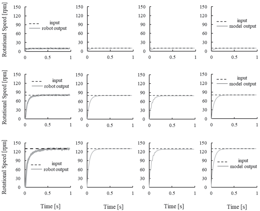
Columns (left to right): robot outputs and those obtained using the method proposed by Nakagawa et al., standard gradient descent, and proposed method. Horizontal axis: time [s], vertical axis: rotational speed [rpm].
Fig. 3. Step responses of the robot and three identified models under step inputs of 10, 80, and 130 rpm.
The settling time of the model obtained using the proposed method was approximately 0.25 s, and the model exhibited an average relative steady-state error of 0.045%. The average relative steady-state error was calculated using Eq. (22).
The optimal value of the objective function \(H(x)\) obtained from the identification experiment was 21.80. The corresponding optimal parameters were as follows:
\(A=0.881\), \(B=-0.151\), \(C=0.122\), \(D=0.0744\), \(E=0.149\), \(F=-0.0748\).
For clarity, the parameter values were rounded off to three significant digits. These parameters were used for the subsequent experiments described in Sections 4.3 and 4.4.
4.2. Comparative Analysis of Method Accuracy
The response data obtained using 13 sets of step signals ranging from 10 to 130 rpm in steps of 10 rpm were used as the test data. For each set, the experiment was repeated five times. For each data group, the following three metrics were used to evaluate the accuracy of the models: relative steady-state error, rise time, and settling time.
The relative steady-state error was calculated using Eq. (22). The rise time was defined as the difference in the time required for the system output to increase from 10% to 90% of the final steady-state value. Settling time is the minimum time required for the system output to enter and remain consistently within a bandwidth of \(\pm 2\)% of the final steady-state value.
The results of the relative steady-state error, rise time, and settling time obtained for the successful models are shown in Fig. 4. The first column shows the values of the three metrics for the robot output, and the next three columns show the three metrics obtained from the model proposed by Nakagawa et al., the standard gradient descent model, and the proposed model.
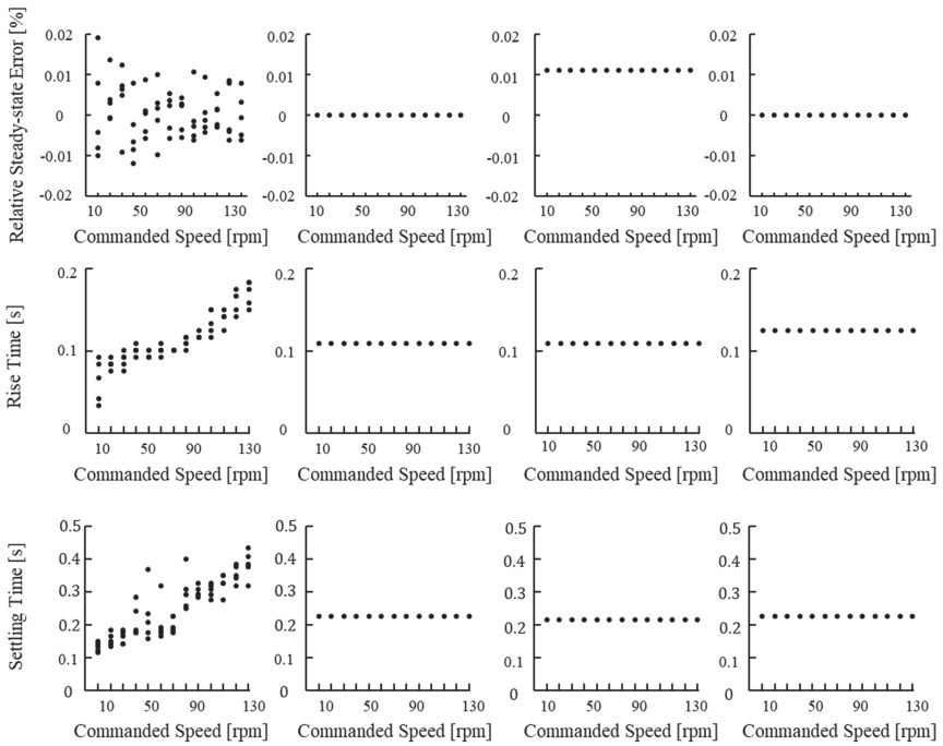
Columns (left to right): robot output; method of Nakagawa et al.; standard gradient descent method; proposed method. Rows (top to bottom): relative steady-state error [%], rise time [s], and settling time [s]. Horizontal axis: commanded speed [rpm], vertical axis: indicated metric value.
Fig. 4. Results on test data arranged in three rows and four columns.
The first row of Fig. 4 compares the relative steady-state errors acquired on the test data.
The relative steady-state errors on robot output show an average of \(4.52\times 10^{-4}\). The model proposed by Nakagawa et al. and the standard gradient descent model exhibit averages of \(2.79\times 10^{-6}\) and 0.0109, respectively. By contrast, the proposed method exhibits an almost zero relative steady-state error of \(-4.41\times 10^{-8}\).
The second row in Fig. 4 shows the rise times. The actual rise time of the robot is approximately 0.11 s. The rise time of the model proposed by Nakagawa et al. and the standard gradient descent model is 0.11 s. The proposed method exhibits a rise time of 0.12 s.
As shown in the third row of Fig. 4, the settling time of the robot is approximately 0.25 s. The settling times of the models presented by Nakagawa et al. and this study are 0.23 s and that of the standard gradient model is 0.22 s. All three methods accurately yielded the step response of the robot.
Nevertheless, the proposed method reduced steady-state error to a near-zero value, while maintaining a dynamic performance comparable to that of the robot.
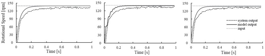
From left to right: model outputs from Nakagawa et al.’s method, standard gradient descent method, proposed method. Horizontal axis: time [s], vertical axis: rotational speed [rpm].
Fig. 5. Step responses of three identified models to a 140-rpm step input.
4.3. Input Tests Beyond Linear Operating Range
The input signal beyond the linear operating range and the response of the target system are shown in Fig. 5. The three response curves of the models for the successful case are shown in the same figure. As observed from the response curve of the target system, the maximum output speed is limited to 135 rpm when the command speed exceeds 135 rpm. This constraint can be incorporated into the model proposed by Nakagawa et al. and the proposed model via programming. The standard gradient descent model exhibits a significant fluctuation in the ascending part of the model response curve, which is also observed for command speeds higher than 110 rpm. This phenomenon leads to faster cumulative errors in response to rapidly changing inputs.
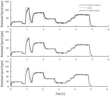
From top to bottom: model outputs from Nakagawa et al.’s method; standard gradient descent method; proposed method. Horizontal axis: time [s], vertical axis: rotational speed [rpm].
Fig. 6. Responses of three model under a random input signal.
4.4. Random Inputs Response
An illustrative five-trial random-input response is shown in Fig. 6. This experiment was conducted to observe the dynamic and steady-state responses of the models. The values of all the inputs were randomly generated. In each experiment, the input design included five cases intended to capture steady-state responses lasting longer than the settling time and five cases intended to capture dynamic responses lasting less than the settling time. Random experiments were conducted five times, with each trial lasting 5.2 s. Table 1 shows the MSE of the model obtained using the three methods in five trials.
Table 1. MSE [rpm\(^2\)] of random input experiments.
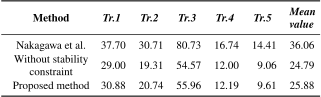
As shown in Table 1 and Fig. 6, the average MSE of the model under stability constraints is only 1.077 rpm\(^2\) larger than that of the model without stability constraints. However, the stability constraints ensure the stability of the obtained model without compromising accuracy. Hence, the obtained model is closer to the actual system in theory. This helps in preventing the identification of unstable models, which may produce gradually diverging outputs even under small initial state perturbations and near-zero inputs over a long simulation time. In addition, the MSE of the proposed model is smaller than that of the model proposed by Nakagawa et al.
As evident from the aforementioned results, the gradient descent method incorporating stability constraints using the Routh–Hurwitz criterion can stabilize the model obtained after parameter estimation by ensuring gradient descent accuracy. However, this can lead to a descent failure owing to the addition of constraints. In successful trials, the models satisfied both the stability conditions and exhibited acceptable accuracy performance. By contrast, the step responses of the models obtained in the unsuccessful cases exhibited highly oscillatory responses or nearly flat outputs with singular spikes. These models exhibited extremely large MSE with respect to the actual outputs and lacked physically meaningful behavior, rendering them unsuitable for control design.
The 60% success rate (Section 4.1) was obtained using different initial values. This indicates that these failures appear to be strongly related to the choice of initial values. This is likely because the feasible regions defined by the Routh–Hurwitz criterion may have nonconvex portions, which may induce the gradient descent algorithm to converge to suboptimal regions. These characteristics can hinder the convergence process and cause the descent process to stagnate or diverge even when the input signals are appropriate. This suggests that the success of the method depends not only on constraint formulation but also on proper initialization strategy. Additionally, repeated trials with different initializations can increase the likelihood of obtaining a valid model. From an engineering perspective, a viable approach is to perform multiple runs and select the converged results for deployment. Future studies should consider improved initialization schemes to enhance the convergence rate of this method.
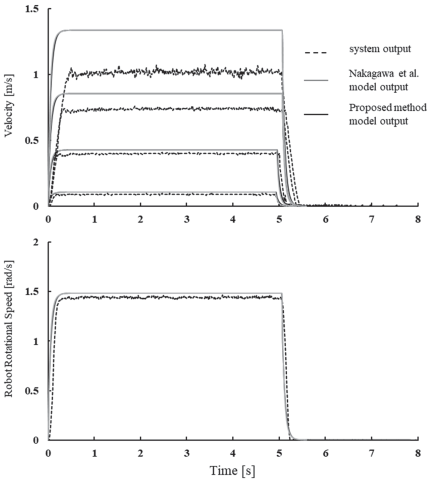
Fig. 7. Comparison of proposed model, Nakagawa et al.’s model, and robot outputs in motion experiments.
4.5. Analysis of Identified Model in Robot Motion Experiments
To evaluate the applicability of the model, a series of speed–response experiments were conducted on a four-wheeled Mecanum robot platform, and its motion characteristics was measured using an MPU9250 sensor. Specifically, the robot was programmed to start from rest and move in a straight line toward the target velocity or rotate in place during the acceleration, steady-state, and deceleration phases. The target velocities were set at 10, 40, 80, and 130 rpm for linear motion and 1.484 rad/s for rotational motion.
Figure 7 shows the proposed model and the model presented by Nakagawa et al. The figure also shows the measured responses of the robot platform during forward motion experiments at different speeds and stationary rotation experiments. As shown in Fig. 7, the overall trends predicted by the proposed model and that presented by Nakagawa et al. align well with the measured data.
However, during the rising phase, the proposed model and that presented by Nakagawa et al. exhibited rising times of 0.12 s and 0.11 s, respectively, both of which were lower than the rising time of the robot platform (0.19 s). During the steady-state phase, the relative steady-state errors at input speeds of 10, 40, 80, and 130 rpm were 0.186, 0.0689, 0.156, and 0.310, respectively. The relative steady-state error at the input rotational speed of 1.484 rad/s was 0.0306. The model output speeds consistently exceeded the measured values.
The maximum relative steady-state error of 0.31 was observed at the speed of 130 rpm, which can be attributed to the output saturation limits of the robot system, which prevent the actual response from scaling further with higher inputs, as mentioned in Section 4.3. The errors at 10, 40, and 80 rpm likely resulted from the system load, rolling friction, and sensor response latency, which were not explicitly modeled at the robot level.
While the proposed model shows satisfactory performance at the wheel level, deviations were observed between the model outputs and robot-level responses, particularly at the steady-state speed and rise time. These results indicate that the models established under no-load conditions exhibit systematic deviations under actual operating conditions. As the focus of this study was to present a system identification method that is feasible under low command-update frequency conditions, our primary objective was to model the core motor dynamics rather than the full robot behavior.
In future studies, we plan to incorporate load modeling, nonlinear friction compensation, and dynamic sensor error correction to enhance the applicability of the model in real-world control systems. Additionally, by collecting response data under various load conditions and integrating real-time modeling with online update mechanisms, the model parameters can be dynamically optimized. This approach improves control reliability and prediction accuracy in complex environments.
4.6. Computational Efficiency Assessment
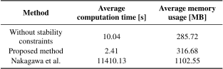
The computational efficiencies of the proposed method, gradient descent method, and the method proposed by Nakagawa et al. were compared. All methods used the same programming language, compiler version, operating system, computer, and modeling data. The average computation times and mean memory usages of the three methods are listed in Table 2. The proposed and gradient descent methods were performed 10 times with different initial parameters. The method presented by Nakagawa et al. was used only five times because of its long computation time, and the mean memory usage of this method was sampled during operation.
As shown in Table 2, the computation time and memory usage of the gradient descent methods are markedly shorter than those of the “exhaustive search method” proposed by Nakagawa et al. Owing to the addition of constraints, the average memory usage of the proposed method is higher than that of the gradient descent method without constraints. Constraint incorporation necessitates additional computations and updating of the Lagrange multipliers during each computation. However, reasonable constraints help narrow the region of feasible solutions, thereby enabling the algorithm to locate the optimal solution faster and reducing the number of unnecessary iterations. Therefore, the average computation time of the proposed method was less than that of gradient descent without constraints.
Table 2. Computational efficiency of methods.
5. Conclusion
In this study, a system identification method based on the system stability criterion was proposed to model a four-wheeled Mecanum robot with an input signal frequency of 10 Hz. The characteristics of the motor and motor driver were unknown. The model consisted of two parts: (1) the kinematic equation between the wheel rotational speed and the overall motion of the robot and (2) the relationship between the input driving signal and the wheel rotational speed, which was represented as a difference equation in this study. By incorporating the Routh–Hurwitz stability criterion, system stability was integrated into the parameter estimation process. The parameters were estimated using the gradient descent method, with the Routh–Hurwitz stability criterion incorporated as a constraint using the KKT conditions to ensure system stability during the estimation process.
To verify the effectiveness of the proposed method, four sets of step-response signals were used as the initial data for parameter estimation, with experiments repeated thrice for each set. The response data consisted of 13 sets of step signals. Experiments were repeated five times for each set to collect the test data and then compare the dynamic and steady-state characteristics of the models obtained with and without stability constraints. These models were also compared with the model proposed by Nakagawa et al. Additionally, five trials of random input experiments were performed to compare the dynamic and steady-state responses of the models obtained using the three methods.
Constraint incorporation led to a decrease in success rate from 90% to 60%, whereas the system stability rate, defined as the ratio of the number of stable models to the total number of parameter estimation trials, increased from 30% to 60%.
The proposed method achieved an almost zero relative steady-state error of \(-4.41\times 10^{-8}\), which was markedly lower than that obtained using the model presented by Nakagawa et al. (\(2.79\times 10^{-6}\)) and standard gradient descent method (\(1.09\times 10^{-2}\)) by 2–5 orders of magnitude. It also maintained competitive dynamic performance with a rise time of 0.12 s and settling time of 0.23 s, closely aligning with the rise time (0.11 s) and settling time of the robot (0.25 s), respectively.
In the random-input experiment, the proposed method maintained the numerical stability of the model under complex and rapidly changing inputs. The average MSE was higher than that observed for the gradient descent method without constraints by approximately 1.077 (in 5.2 s). However, this loss of accuracy was minimal. The average MSE obtained using the method proposed by Nakagawa et al. was higher than that observed for our method, indicating that the former is not as robust as the proposed method when handling rapidly changing inputs.
The above experiments indicated that the gradient descent method considering stability constraints based on the Routh–Hurwitz criterion can stabilize the model obtained after parameter estimation by ensuring gradient descent accuracy. However, owing to the nonconvex portions of the feasible regions, success rate is sensitive to the choice of initial values. Multiple trials are required to identify viable results for engineering deployment.
To validate the applicability of the proposed model to real-world robot motion, a four-wheeled Mecanum robot platform was moved in a straight trajectory at different speeds and rotated in place. The results indicated that the overall trends of the proposed model aligned well with the measured data. However, systematic deviations were observed in the steady-state velocity and rise time owing to unmodelled load effects and friction. These findings suggest that the proposed model is effective under no-load identification conditions. Future studies will incorporate load modeling, nonlinear friction compensation, and sensor error correction to improve robot-level reliability. In addition, the practical applicability of the model in situations involving frequent transitions between forward and reverse wheel rotations will be considered. Such cases may introduce asymmetric behavior owing to accumulated mechanical backlash, uneven gear responses, or other structural nonlinearities, reducing the accuracy of the wheel-level model in Eq. (2). Addressing these effects is essential for the practical applicability of the models obtained using the proposed method.
Finally, the computational efficiencies of the proposed method, gradient descent method, and the method proposed by Nakagawa et al. were compared. The proposed method achieved the lowest computation time among the three methods. Although its memory usage is higher than that of the gradient descent method, it does not affect the computation speed provided there is sufficient memory.
These results indicate the effectiveness of introducing stability constraints into parameter estimation for limiting input signal frequency systems, ensuring accuracy, system stability, and computational efficiency.
Acknowledgments
Part of this work was supported by the Sciences Research Grants of the Ministry of Education, Culture, Sports, Science, and Technology (Grant Numbers: 16K12199 and 22K12106). Part of this work was commissioned by the Ministry of Internal Affairs and Communications under SCOPE (Reference Number: 181603016). The authors are grateful for the support.
- [1] M. Nakamura and K. Hoshino, “Experimental discussion about the influence of the proficiency in Tankendo in the foot posture,” Humanities & Social Sciences Reviews, Vol.7, No.5, pp. 296-305, 2019.
- [2] K. Hoshino, Y. Ozone, and C. Zhao, “A Tankendo robot that defends itself from opponent attacks by moving immediately before a valid strike or thrust: A Tankendo robot defends from opponent attacks,” Proc. of the 2021 3rd Int. Conf. on Image, Video and Signal Processing (IVSP’21), pp. 115-121, 2021. https://doi.org/10.1145/3459212.3459230
- [3] K. Hoshino, Y. Noguchi, Y. Nakai, Y. Ozone, and M. Nakamura, “Predicting the types of striking and thrusting motions by using deep learning,” 2019 6th Int. Conf. on Biomedical and Bioinformatics Engineering (ICBBE’19), pp. 199-202, 2019. https://doi.org/10.1145/3375923.3375954
- [4] Y. Ozone, C. Zhao, and K. Hoshino, “Introducing swordsman robot defensing,” 2020 3rd Int. Conf. on Digital Medicine and Image Processing (DMIP’20), pp. 33-39, 2020. https://doi.org/10.1145/3441369.3441375
- [5] H. Mitsuhashi, T. Kodama, and T. Itami, “Real-time stair angle estimation based on 3D dynamic analysis for an omnidirectional autonomous electric wheelchair realizing illuminance-independent multiple obstacle detection and stair climbing,” J. Robot. Mechatron., Vol.37, No.6, pp. 1602-1618, 2025. https://doi.org/10.20965/jrm.2025.p1602
- [6] R. Miura, S. Tozaki, I. Mikado, T. Takei, S. Ogake, K. Kobayashi, S. Mitsui, T. Satake, and N. Igo, “Development of a decommissioning robot with a simple structure capable of traversing steps using two different drive systems,” J. Robot. Mechatron., Vol.36, No.1, pp. 95-106, 2024. https://doi.org/10.20965/jrm.2024.p0095
- [7] G. Cao, X. Zhao, C. Ye, S. Yu, B. Li, and C. Jiang, “Fuzzy adaptive PID control method for multi-Mecanum-wheeled mobile robot,” J. of Mechanical Science and Technology, Vol.36, pp. 2019-2029, 2022. https://doi.org/10.1007/s12206-022-0337-x
- [8] C. Tezel and G. Bayar, “Theoretical and experimental investigation of variable contact forces on the rollers of a Mecanum wheeled mobile robot,” The Int. J. of Robotics Research, Vol.43, No.8, pp. 1208-1227, 2024. https://doi.org/10.1177/02783649241228607
- [9] M. Szeremeta and M. Szuster, “Neural tracking control of a four-wheeled mobile robot with Mecanum wheels,” Applied Sciences, Vol.12, No.11, Article No.5322, 2022. https://doi.org/10.3390/app12115322
- [10] Y. Nakagawa, N. Igo, and K. Hoshino, “Controlling a Mecanum-wheeled robot with multiple Swivel axes controlled by three commands,” Sensors, Vol.25, No.3, Article No.709, 2025. https://doi.org/10.3390/s25030709
- [11] L. Ljung, “System identification: Theory for the user (2nd ed.),” pp. 8-14, Prentice Hall, 1999.
- [12] H. Masood, A. Zafar, M. U. Ali, T. Hussain, M. A. Khan, U. Tariq, and R. Damaševičius, “Tracking of a fixed-shape moving object based on the gradient descent method,” Sensors, Vol.22, No.3, Article No.1098, 2022. https://doi.org/10.3390/s22031098
- [13] J. Wang, Q. Hou, Z. Zhuo, H. Jia, and N. Zhang, “Voltage stability constrained economic dispatch for multi-infeed HVDC power systems,” IEEE Trans. on Power Systems, Vol.39, No.2, pp. 2598-2610, 2024. https://doi.org/10.1109/tpwrs.2023.3277213
- [14] Y. Tian, Y. Zhang, and H. Zhang, “Recent advances in stochastic gradient descent in deep learning,” Mathematics, Vol.11, No.3, Article No.682, 2023. https://doi.org/10.3390/math11030682
- [15] F. Le and S. Dong, “Performance improvements in natural gradient descent method,” 2024 7th Int. Conf. on Advanced Algorithms and Control Engineering (ICAACE), pp. 1089-1092, 2024. https://doi.org/10.1109/icaace61206.2024.10549159
- [16] R. Chen, X. Tang, and X. Li, “Adaptive stochastic gradient descent method for convex and non-convex optimization,” Fractal and Fractional, Vol.6, No.12, Article No.709, 2022. https://doi.org/10.3390/fractalfract6120709
- [17] S. H. Haji and A. M. Abdulazeez, “Comparison of optimization techniques based on gradient descent algorithm: A review,” PalArch’s J. of Archaeology of Egypt/Egyptology, Vol.18, No.4, pp. 2715-2743, 2021.
- [18] C. Zhao, T. Shibuya, N. Igo, and K. Hoshino, “Method of controlling a Tankendo robot using a Mecanum wheel trolley robot,” 2022 7th Int. Conf. on Intelligent Information Technology (ICIIT 2022), pp. 126-130, 2022. https://doi.org/10.1145/3524889.3524910
- [19] H. Taheri, B. Qiao, and N. Ghaeminezhad, “Kinematic model of a four Mecanum wheeled mobile robot,” Int. J. of Computer Applications, Vol.113, No.3, pp. 6-9, 2015. https://doi.org/10.5120/19804-1586
- [20] M. Hamaguchi, “Damping and transport control of a spherical pendulum on an omnidirectional wheeled robot during manual operation,” J. Robot. Mechatron., Vol.37, No.6, pp. 1410-1419, 2025. https://doi.org/10.20965/jrm.2025.p1410
- [21] M. Kuczmann, “Review of DC motor modeling and linear control: Theory with laboratory tests,” Electronics, Vol.13, No.11, Article No.2225, 2024. https://doi.org/10.3390/electronics13112225
- [22] C. L. Phillips and T. Nagle, “Digital control system analysis and design (3rd ed.),” pp. 234-239, Prentice Hall, 1995.
- [23] S. Boyd and L. Vandenberghe, “Convex optimization,” pp. 215-231, Cambridge University Press, 2004. https://doi.org/10.1017/cbo9780511804441
- [24] Y. Nesterov, “Introductory lectures on convex optimization: A basic course (1st ed.),” pp. 22-26, Kluwer Academic Publishers, 2004.
- [25] H. H. Bauschke and P. L. Combettes, “Convex analysis and monotone operator theory in Hilbert spaces (1st ed.),” pp. 43-52, Springer, 2011. https://doi.org/10.1007/978-1-4419-9467-7
This article is published under a Creative Commons Attribution-NoDerivatives 4.0 Internationa License.