Paper:
Soil-Adaptive Autonomous Excavation: Bulking Factor-Based Soil Density Estimation and Excavation Path Optimization with a Genetic Algorithm
Ryosuke Yajima*1, Shinya Katsuma*1, Shunsuke Hamasaki*2, Pang-jo Chun*1
 , Keiji Nagatani*1,*3
, Genki Yamauchi*4
, Takeshi Hashimoto*4
, Atsushi Yamashita*5
, and Hajime Asama*6
, Keiji Nagatani*1,*3
, Genki Yamauchi*4
, Takeshi Hashimoto*4
, Atsushi Yamashita*5
, and Hajime Asama*6
*1Graduate School of Engineering, The University of Tokyo
7-3-1 Hongo, Bunkyo-ku, Tokyo 113-8656, Japan
*2Faculty of Science and Engineering, Chuo University
1-13-27 Kasuga, Bunkyo-ku, Tokyo 112-8551, Japan
*3Faculty of Systems and Information Engineering, University of Tsukuba
1-1-1 Tennodai, Tsukuba, Ibaraki 305-8577, Japan
*4Public Works Research Institute
1-6 Minamihara, Tsukuba, Ibaraki 305-8516, Japan
*5Graduate School of Frontier Sciences, The University of Tokyo
5-1-5 Kashiwanoha, Kashiwa, Chiba 277-8561, Japan
*6Tokyo College, Institutes for Advanced Study, The University of Tokyo
7-3-1 Hongo, Bunkyo-ku, Tokyo 113-8656, Japan

In this study, we present a novel autonomous excavation method that achieves high efficiency under varying soil conditions. This method consists of two main steps, including first estimating the density of the soil and then generating an optimal excavation path based on the estimated density. The proposed method estimates soil density by taking advantage of the bulking phenomenon, which refers to an increase in the volume of excavated soil. This estimation relies solely on 3D point-cloud data obtained before and after excavation. Using the estimated soil density, an optimal excavation path is generated by applying a genetic algorithm in a physics simulator that replicates both the hydraulic excavator and the target ground. The algorithm explores a range of paths over multiple generations to find one that maximizes efficiency. The effectiveness of the proposed method was verified through simulations and field experiments. In particular, field experiments conducted in soft soil showed that the proposed method improved excavation efficiency by 27.7% compared with a baseline method using fixed parameters.
Autonomous excavation planning method
1. Introduction
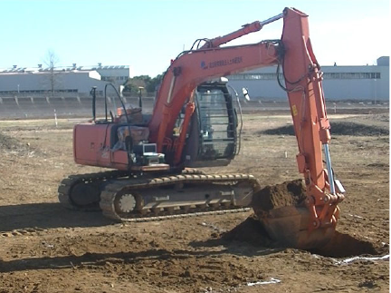
Fig. 1. A hydraulic excavator. Hydraulic excavators are commonly used on construction sites. An excavator consists of a lower frame and an upper frame equipped with a front attachment.
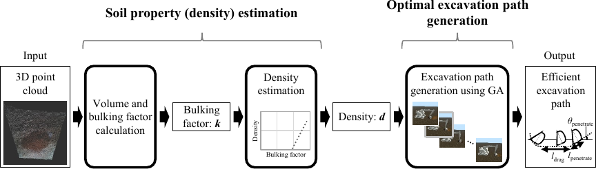
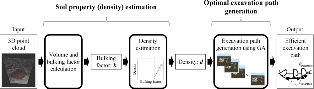
Fig. 2. Overview of the proposed autonomous excavation planning method. The method consists of two main components, including estimation of soil properties and generation of an optimal excavation path based on the estimated properties.
Automation of construction machinery is in high demand, given that the construction industry has been striving to improve its labor-intensive processes over the past several decades 1. Hydraulic excavators are among the most widely used machines on construction sites, as illustrated in Fig. 1. Although operating hydraulic excavators requires considerable skill and experience, the number of such skilled operators is decreasing in rapidly aging countries 2. Therefore, the development of autonomous excavation methods that can match the efficiency of skilled operators is essential.
Because the soil conditions at construction sites vary significantly from location to location, autonomous excavators must achieve high efficiency across different types of soil. High efficiency refers to the ability to excavate large volumes of soil while consuming less energy. Numerous studies have been conducted to realize autonomous excavation 3,4,5. However, most autonomous excavation methods either did not consider soil information or assumed that it was known beforehand. Consequently, they were unable to achieve high efficiency under the varying soil conditions that obtain on actual construction sites.
Two types of soil information are primarily considered in certain autonomous excavation methods, including the shape of the soil pile and its properties (e.g., density). With respect to the shape of the target soil pile, several studies have attempted to incorporate shape information in autonomous excavation 6. These studies measured the shape of a soil pile using 3D point-cloud data and utilized it to plan multiple excavation cycles (e.g., determining where to start an excavation cycle). However, these studies assumed that soil properties were known beforehand. When soil properties cannot be obtained beforehand or differ from assumed values, these methods fail to achieve high efficiency. Moreover, a data-driven approach has been proposed that utilizes the shape of the soil surface to control excavation such that the bucket filling ratio reaches a desired target 7. Although the bucket filling ratio is related to fuel efficiency, this approach indirectly considers efficiency, which is not directly evaluated.
On the other hand, several previous studies have attempted to measure soil properties for autonomous excavation 8,9. Fundamentally, these studies rely on force sensors because they utilize models of soil dynamics such as the fundamental equation of earth-moving mechanics 10 or its variants 11. A recent survey of work on autonomous excavators also reviewed studies on soil parameter estimation; however, these methods similarly rely on force measurements 12. However, installing force sensors in conventional excavators is not straightforward. These points highlight the need for a method that can easily obtain soil properties and perform excavation autonomously based on that information. Recently, payload- and force-estimation functions have been introduced in some commercial excavators. However, demand for further automating conventional machines without such functions is expected to continue, and alternative approaches are called for.
In this study, we developed a more practical autonomous excavation method by utilizing soil properties. To achieve this objective, we developed a novel method to estimate soil density as a representative soil property using only 3D point-cloud data by focusing on the bulking of excavated soil. Furthermore, we established a method to identify efficient excavation paths under varying soil conditions by using a genetic algorithm (GA) and a physical simulator.
The remainder of this study is organized as follows. In Section 2, we describe the proposed method in detail. Section 3 presents simulation experiments conducted to validate the effectiveness of the proposed method. Section 4 describes field experiments conducted using a real hydraulic excavator. Finally, we conclude in Section 5 by suggesting some possible avenues for further research.
2. Proposed Method
2.1. Overview
The proposed method considers the density of the target soil to estimate its properties and perform autonomous excavation based on that information. Density significantly influences the penetration resistance of soil13,14, which is critical in planning an excavation. In this study, we proposes a method to estimate soil density from 3D point-cloud data and generate optimal excavation path parameters based on the estimated density. An overview of the proposed method is presented in Fig. 2. The flow of the main process is as follows.
-
3D point-cloud data of the ground before and after excavation are obtained.
-
The volume of the soil pile before and after excavation is calculated using the 3D point cloud data.
-
The bulking factor of soil is calculated from the volume.
-
The soil density is estimated from the bulking factor of the soil using a relational expression.
-
Soil with the estimated density is replicated in a physical simulator.
-
Optimal excavation path parameters for the soil are obtained using the simulator.
-
An automated excavator excavates the ground along the excavation path defined by the obtained path parameters.
Note that this method must be applied in a repeated excavation cycle because it requires 3D point-cloud data about the ground before and after excavation. Moreover, the method assumes that the current excavation point is close to the previous one and that their soil properties are nearly identical. Although the proposed method includes searching for an excavation path using a simulator, that would be too time-consuming in practical applications. Realistically, we consider that searching for candidate optimal excavation paths in advance for multiple expected soil conditions using the simulator as a preliminary process and then selecting the most appropriate path based on the estimated soil properties during excavation would be more practical.
Items 1–4 correspond to soil property estimation, whereas items 5–7 correspond to optimal path generation and autonomous excavation. In the estimation process, the input is a 3D point-cloud data of the target ground, and the output is the estimated soil density. In the path generation process, the input is the estimated soil density and the output is the optimal parameters representing an excavation path. Details of each process are provided in the following sections.
2.2. Soil Density Estimation Based on the Bulking Factor Using 3D Point-Cloud Data
2.2.1. Basic Principle of Soil Density Estimation
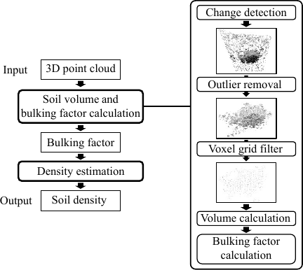
Fig. 3. Procedure for estimating soil density. After processing the point clouds, the soil volume and the bulking factor are calculated, and the soil density is subsequently estimated based on the bulking factor.
As mentioned above, soil density affects penetration resistance, which is critical in excavation planning. In general, direct measurement methods such as the core method are used to determine soil density at construction sites. However, these methods are not applicable during the excavation process because they are time-consuming and destructive 15. Therefore, we propose a new method here to measure or estimate soil density during the excavation process.
To estimate soil density, we focused on the bulking factor of the soil. Bulking factor is an indicator of the increase in soil volume that occurs during the excavation process 16. Soil volume increases after excavation due to changes in the structure of the soil that create additional void space. Experimental works have established that the bulking factor and soil density exhibit a strong positive correlation 17. Qualitatively, a large bulking factor indicates that the soil is dense and hard. Moreover, the soil volumes before and after excavation, which are necessary to calculate the bulking factor, can be derived from 3D point-cloud data acquired using sensors that are relatively easy to install such as LiDAR or RGB-D sensors. In particular, many studies have explored the use of RGB-D sensors on construction sites 18,19,20. Thus, in this study, we calculated the bulking factor from 3D point-cloud data and estimated soil density based on the bulking factor. The procedure used to estimate the density of the soil is summarized in Fig. 3. The details of each step are described below.
2.2.2. Calculation of Soil Volume and Bulking Factor Using 3D Point-Cloud Data
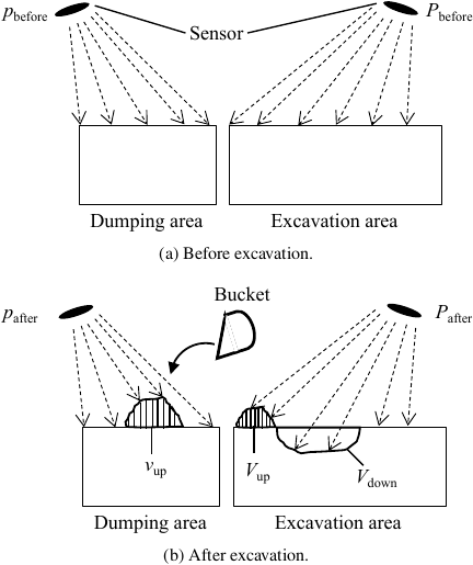
Fig. 4. Measurement method for the bulking factor. The volumes of excavated and dumped soil are calculated from 3D point clouds of the ground surface obtained using RGB-D sensors or equivalent devices.
First, the soil volume and bulking factor are calculated using 3D point-cloud data.
The bulking factor quantifies the increase in soil volume. Let \(k\) denote the bulking factor. It is defined as follows.
The system shown in Fig. 4 is used to calculate the volume of the soil. As shown in the figure, two areas are measured, including the excavation and dumping areas. 3D point-cloud data are obtained from each area.
-
\(P_{\rm{before}}\): 3D point-cloud data of the excavation area before excavation.
-
\(P_{\rm{after}}\): 3D point-cloud data of the excavation area after excavation.
-
\(p_{\rm{before}}\): 3D point-cloud data of the dumping area before excavation.
-
\(p_{\rm{after}}\): 3D point-cloud data of the dumping area after excavation.
The proposed method calculates the following three soil volumes from the 3D point-cloud data, as illustrated in Fig. 4.
-
\(V_{\rm{up}}\): The volume of spilled soil.
-
\(V_{\rm{down}}\): The volume of excavated soil.
-
\(v_{\rm{up}}\): The volume of dumped soil.
The point cloud is processed for this calculation. First, changes in the 3D point-cloud data before and after excavation are detected. Subsequently, outliers in the point cloud are removed. Then, a voxel grid filter is applied to the point cloud. After applying the voxel grid filter, let the \(i\)-th point of the processed point cloud be \(p_i = (x_i, y_i, z_i)\). The soil volumes are then calculated as
2.2.3. Estimation of Soil Density Based on the Bulking Factor
Next, soil density is calculated based on the bulking factor.
In this study, we consider the relative soil density \(d\), which is defined as follows.
As noted above, it has been demonstrated experimentally that the bulking factor and soil density exhibit a strong positive correlation 17. Soil with higher density exhibits a larger bulking factor, whereas soil with lower density exhibits a smaller bulking factor. Therefore, the relationship between density \(d\) and bulking factor \(k\) is assumed to be linear, as expressed by the following equation.
2.3. Generating Efficient Excavation Paths Based on Estimated Soil Density
2.3.1. Efficiency of Excavation
An objective function is required to generate an optimal excavation path. Here, we focused on the efficiency of excavation. The efficiency of excavation \(f\) is defined as follows.
2.3.2. Representation of Excavation Path
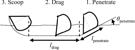
Fig. 5. Modeled excavation path based on expert excavator operations. The path consists of a penetration phase, a dragging phase, and a scooping phase, and can be described using three parameters.
The proposed method applies an excavation path represented by a set of parameters. We consider an excavation path represented by three parameters as shown in Fig. 5. This path is based on excavation operations performed by experienced operators. Several studies have investigated excavation operations performed by experienced operators 21,22. In general, such operations can be divided into three phases, including penetrating, dragging, and scooping. In the penetration phase, operators insert the bucket into the target soil until it reaches the bottom line of the desired excavation area while keeping the bottom of the bucket parallel to the penetration line to minimize resistance force. Subsequently, in the dragging phase, the tip of the bucket is dragged horizontally along the bottom line while maintaining a fixed angle between the bucket and the arm. Finally, in the scooping phase, the operators rotate only the bucket until it is oriented horizontally. To model these operations, we consider the following three parameters.
-
\(\theta_{\rm{penetrate}}\): The angle between the horizontal surface and the penetration line.
-
\(l_{\rm{penetrate}}\): The length of the penetration line.
-
\(l_{\rm{drag}}\): The length of the dragging line.
These parameters determine the bucket posture at a given moment, which in turn determines the joint angles of the boom, arm, and bucket. Excavation along the planned path can be carried out by controlling each joint according to these parameters.
In this study, we made two assumptions regarding the excavation model. First, we assumed that the excavator does not move laterally while the bucket is in contact with the ground. This implies that the excavation model considers only the \(XZ\) plane. Second, we assumed that the position of the main body of the excavator is fixed.
2.3.3. Generation of Optimal Excavation Path Using a GA
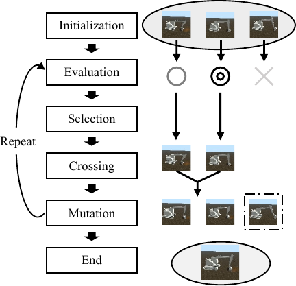
Fig. 6. Concept of optimal excavation path search using a GA. An optimal path is obtained by testing various excavation paths over a predefined number of generations on a physics simulator that replicates the hydraulic excavator and the target soil.
Finally, an efficient excavation path is generated for the target soil. Thus, our approach finds the values of three parameters that represent an excavation path with the highest efficiency for soil of a given density.
To that end, the proposed method searches for an excavation path by applying a GA 23. The GA is an evolutionary optimization algorithm inspired by natural selection. At each generation \(t\), a population of candidate solutions \(\{ x_1^t, x_2^t, \dots, x_N^t \}\) is maintained. The quality of each individual \(x_i^t\) is evaluated using a fitness function \(f(x_i^t)\). Individuals with higher fitness values are more likely to be selected as parents and new individuals are generated through crossover and mutation to form the next generation \(\{ x_1^{t+1}, x_2^{t+1}, \dots, x_N^{t+1} \}\). Through this iterative process, the population converges toward an optimal or nearly optimal solution without requiring gradient information. The GA is suitable for this study because the gradient of the excavation efficiency cannot be calculated.
Figure 6 illustrates the concept of searching for an optimal excavation path using a GA. In this method, the GA searches for the best excavation path by testing various paths over a pre-defined number of generations using a physics simulator that replicates the hydraulic excavator and the target soil. The fitness function of each individual is defined by the excavation efficiency \(f\) as described above. Therefore, the GA is expected to return an efficient excavation path that minimizes energy consumption while maximizing the amount of excavated soil.
In this study, each individual in the GA population was represented as a vector of the following three parameters. \((\theta_{\text{penetrate}}, l_{\text{penetrate}}, \textrm{and}~l_{\text{drag}})\), respectively represent the angle and length of penetration and the dragging length of the excavation path. In the initialization step, these parameters are assigned random values within specified ranges such that each individual corresponds to a distinct excavation motion. The fitness of each individual is then calculated using the excavation efficiency \(f\) defined above. To generate the next generation, the elitism and tournament selection methods are combined. In elitism, the best individual of the current generation is directly preserved in the next generation. For tournament selection, a small group of individuals is randomly sampled from the remaining population and the one with the highest fitness among them is copied into the next generation. Selected parents undergo crossover using a two-point recombination scheme in which contiguous segments of their parameter vectors are exchanged. After crossover, mutation is applied by randomly altering one or more parameters within their predefined ranges to maintain population diversity and prevent premature convergence. After a predefined number of generations, the individual with the highest fitness is taken as the optimal excavation path.
As mentioned above, it is considered practical to precompute candidate excavation paths for multiple expected soil conditions using this method. In actual operations, excavation can be performed without delay by selecting an optimal excavation path from the precomputed candidates based on the estimated soil density.
3. Simulation Experiments
3.1. Experimental Setting
Table 1. Conditions of soil.

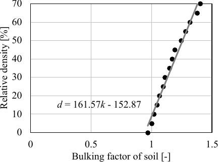
Fig. 7. Relationship between the bulking factor and the soil density. This is based on the results of preliminary experiments in which the excavator model excavated the soil while changing the relative density in increments of 5% in the dynamic simulator.
Simulations were conducted to evaluate the effectiveness of the proposed method.
In the experiments, we used the dynamic simulator Vortex Studio developed by CM Labs Simulations. Vortex Studio enables the replication of soil–tool interactions during the excavation process, which allows the mass of excavated soil and energy consumption to be evaluated. This simulator has been evaluated in a previous study in which soil behavior such as the angle of repose was reproduced 24. In the simulator, an excavator model performed autonomous excavation operations. The model was based on the ZAXIS120 developed by Hitachi Construction Machinery, and was identical to the excavator used in the field experiments. Three soil density conditions were prepared, including soft, medium, and hard soil, as shown in Table 1. The soil type was set to loam, which was the same as that used in the field experiments. In addition, the initial ground surface was set to be flat. Using these settings, the excavation efficiency of the proposed method, which considers the bulking factor of the soil, was compared with that of excavation using fixed parameters. For the fixed parameters, \([\theta_{\rm{penetrate}}, l_{\rm{penetrate}}, l_{\rm{drag}}]\) were set to \([\pi/4, 0.35, 1.5]\). These values were determined empirically to ensure that a sufficient excavation volume was obtained to calculate the bulking factor.
Table 2. Conditions of the GA.

Table 3. Lower and upper limits of genes for each individual.

The relationship between the bulking factor and soil density was determined in advance in the dynamic simulator. Fig. 7 shows the results of the preliminary experiment along with the regression line. The parameters in Eq. \(\eqref{eq:density}\) were determined as \(a = 161.57\) and \(b = -152.87\). Given that the coefficient of determination was \(R^2 = 0.9811\), estimating the soil density from the bulking factor using a linear function did not pose a significant problem.
Candidates for efficient excavation paths were precomputed using the GA in the simulator. The conditions for the GA are listed in Table 2 and the lower and upper bounds of the genes for each individual are given in Table 3. The number of generations was set to be relatively small due to computational time constraints and to obtain reasonable results within the available resources. Under these settings, candidates for efficient excavation paths were obtained for all density patterns ranging from 0% to 100% in continuous increments of 5%.
The detailed procedure for the simulation experiments is as follows.
-
The target ground is excavated once using fixed parameters.
-
The bulking factor is calculated using the height map of the target ground obtained directly from the simulator, instead of point cloud data obtained from RGB-D sensors or similar devices.
-
An efficient excavation path is selected based on the soil density estimated from the bulking factor.
-
The target ground is excavated again using the selected efficient excavation path.
3.2. Experimental Results
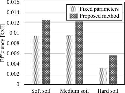
Fig. 8. Experimental results for excavation efficiency in the simulation experiments. The proposed method improves excavation efficiency under all soil conditions.
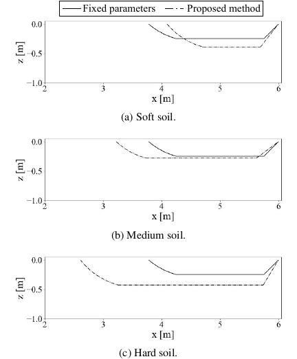
Fig. 9. Excavation paths in the simulation experiments. Using the proposed method, different paths from those with fixed parameters are selected, and the selected paths vary depending on each soil condition.
Figure 8 shows the experimental results for excavation efficiency under the three conditions. For each condition, the left bar represents the excavation efficiency using fixed parameters, while the right bar represents the excavation efficiency using the proposed method. As shown in Fig. 8, the proposed method improved excavation efficiency under all conditions. These results confirm the validity of the proposed method in the simulation environment.
For further discussion, Fig. 9 presents a comparison of the excavation paths. In each figure, the solid line represents the path of the bucket tip with fixed parameters, while the dashed line represents the path of the bucket tip generated by the proposed method. Here, \(x = 0\) is defined as the \(x\)-coordinate of the joint between the base and boom links. Similarly, \(z = 0\) is defined as the \(z\)-coordinate of the initial ground surface. As shown in Fig. 9, the excavation paths generated by the proposed method are adapted to each condition. In particular, it may be observed that the excavation area became larger as the target soil became harder. This result may be related to the definition of excavation efficiency used in this work, in which both the excavated volume and energy consumption are considered. For hard soil, the optimization may have selected a deeper and longer path to compensate for the larger energy required in penetration by increasing the excavated volume. This phenomenon will be addressed in more detail in future work.
4. Field Experiments
4.1. Experimental Setup
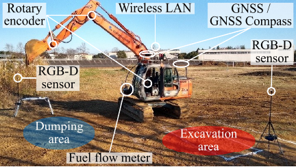
Fig. 10. Field experiment setup. The excavator was automatically controlled. The excavating and dumping areas were placed around the excavator, and RGB-D sensors were installed to obtain 3D point clouds of each area.
Field experiments were conducted to evaluate the proposed method for actual excavators. Fig. 10 shows the experimental setup used in the field experiments.
In this experiment, we used a ZAXIS120 hydraulic excavator developed by Hitachi Construction Machinery. It was equipped with three rotary encoders, including a GNSS, a GNSS compass, a fuel flow meter, and a wireless LAN. The control input to operate the excavator can be transmitted via a wireless connection. The electromagnetic proportional valves of the hydraulic cylinders were opened or closed based on the input. Therefore, the excavator was automatically controlled by transmitting the appropriate input via a wireless connection. This system was implemented using robot operating system (ROS) a. Using this system, an excavator can excavate a predetermined path. For external sensing, we used an Intel RealSense depth camera D435i, developed by Intel, as an RGB-D sensor.
The soil type was loam and the initial ground surface was leveled to be almost flat. The experiment was conducted under two soil conditions, including soft and hard soil. The hardness of the soil was verified in advance using the coefficient of subgrade reaction. Table 4 shows the coefficients of subgrade reaction for each condition measured using a falling weight deflectometer. A larger coefficient of subgrade reaction indicates harder soil. In addition, the same relationship between the bulking factor and soil density described in Section 3 was applied here.
Table 4. Two conditions of soil for the field experiments.

Two types of excavation paths were used, including a fixed-parameter path and an efficient path generated using the proposed method. The fixed-parameter path was used to estimate the soil density and for comparison with the proposed method. For the fixed parameters, \([\theta_{\rm{penetrate}}, l_{\rm{penetrate}}, l_{\rm{drag}}]\) were set to \([1.023, 0.496, 2.487]\), respectively. The parameters were changed from those used in the simulation experiments to ensure a sufficient volume of excavated soil to calculate the bulking factor. When using the same fixed parameters as in the simulation experiments, the volume of the excavated soil was sometimes insufficient due to the roughness of the ground surface and other factors. The same candidate excavation paths used in Section 3 were applied in this experiment. When the estimation of the soil density was sufficiently accurate, an efficient excavation path was selected based on the estimated density. An excavation was performed in an adjacent area where the soil conditions were confirmed to match those of the area used for the fixed-parameter path.
Although the mass of the soil and the energy consumption are necessary to calculate efficiency as shown in Eq. \(\eqref{eq:eq21}\), measuring them directly can be difficult. Thus, the volume of soil accumulated in the bucket after excavation was used instead of the mass of the soil. The volume corresponds to the mass by multiplying it by the density, which was measured using the RGB-D sensor. Similarly, fuel consumption was used instead of energy consumption. Energy consumption can be calculated from fuel consumption and energy density. A fuel flow meter was mounted on the excavator to measure fuel consumption during the excavation process. The total fuel consumption was calculated by integrating the instantaneous flow rate over time because the meter was able to measure the instantaneous rate of fuel flow.
The detailed procedure for the field experiments is as follows.
-
The excavator executes an excavation path using fixed parameters.
-
The bulking factor is calculated from the 3D point-cloud data obtained by the RGB-D sensors.
-
An efficient excavation path is selected based on the soil density estimated from the bulking factor.
-
The target ground is excavated again using the selected excavation path.
-
The total energy consumption during each excavation process and the soil volume accumulated in the bucket are measured, and the excavation efficiency is calculated based on these data.
4.2. Experimental Results on Soil Density Estimation
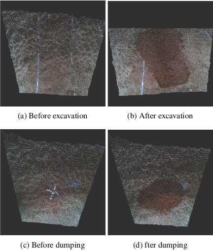
Fig. 11. 3D point-cloud data obtained in the field experiments (soft soil). Dark-colored points in the centers of (b) and (d) indicate the excavated and dumped soil.
First, the experimental results under the soft soil conditions are presented. Fig. 11 shows the 3D point-cloud data measured by the RGB-D sensors during excavation with fixed parameters. In this figure, (a) and (b) show the excavation areas before and after excavation, respectively, and (c) and (d) show the dumping areas before and after dumping. Table 5 lists the bulking factor and the estimated soil density calculated from the 3D point cloud data. As shown in Table 5, a reasonable value was obtained for soft soil.
Here, we consider the experimental results for the hard soil. Fig. 12 shows the 3D point-cloud data measured by the RGB-D sensors during excavation with fixed parameters. Table 5 lists the bulking factor and the estimated soil density calculated from the 3D point-cloud data mentioned above. As shown in Table 5, the estimated density exceeded 100%, although it was theoretically defined to range from 0% to 100%. Based on observations from this experiment, we hypothesized that the presence of compacted soil in the target ground caused this issue. Fig. 13 shows the excavated area of the hard soil. As shown in Fig. 13, a significant amount of compacted soil remained in block-like forms. Given that the compacted soil did not break apart even after excavation, large voids remained in the soil. Because the proposed method assumes that there are no large voids in the soil in the volume calculation, the experimental results overestimated the post-excavation soil volume and underestimated the pre-excavation volume. Consequently, the estimated density exceeded 100%.
Table 5. Measured bulking factor and estimated soil density in the field experiments.

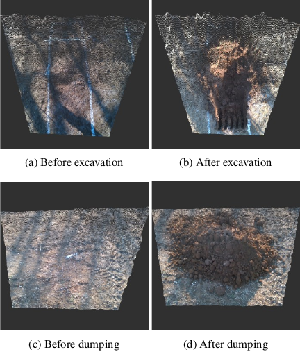
Fig. 12. 3D point-cloud data obtained in the field experiments (hard soil). Dark-colored points in the centers of (b) and (d) indicate the excavated and dumped soil.
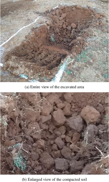
Fig. 13. Ground condition after excavating hard soil. The soil did not collapse during excavation and formed block-like shapes, which affected the calculation of the bulking factor and the estimation of soil density.
4.3. Experimental Results on Efficient Excavation
Based on the results of our estimation of soil density, an efficient excavation was conducted on the soft soil where a valid estimation result was obtained.
Table 6 shows the soil volume accumulated in the bucket after excavation (\(V_{\rm{d}}\)), the total energy consumption during the excavation process (\(E\)), and the excavation efficiency (\(V_{\rm{d}}/E\)). As shown in Table 6, the excavation efficiency using the proposed method was 0.212 \(\rm{m^3}/\rm{mL}\), whereas that obtained using fixed parameters was 0.166 \(\rm{m^3}/\rm{mL}\). This indicates that the proposed method achieved 27.7% higher excavation efficiency than the fixed-parameter approach. Specifically, the proposed method significantly reduced the energy consumption while excavating a similar volume of soil.
Figure 14 compares the fuel flow rates during the excavation process using fixed parameters and the proposed method. The gray line represents the fuel flow rate with fixed parameters, and the black line represents the fuel flow rate with the proposed method. As shown in Fig. 14, the proposed method required less energy during the excavation process. This occurred primarily because the proposed method shortened the dragging phase, which corresponds to the significant gap observed between 5,000 ms and 10,000 ms in Fig. 14.
5. Conclusion
In this study, we have presented an autonomous excavation method capable of achieving high efficiency across different types of soil. To achieve this, we have proposed a novel excavation planning method based on measuring the bulking factor of soil. The novelty of the proposed method lies in its focus on the phenomenon of increased soil volume after excavation. By focusing on the increase in soil volume, the density of the soil can be estimated using only 3D point-cloud data. Furthermore, we have provided a method to generate the most efficient excavation path for a given soil density using a GA. The validity of the proposed method was confirmed through the results of both simulations and field experiments.
Table 6. Excavation efficiency results in the field experiments (soft soil).

Future work should consider improving robustness to the presence of compacted soil in the ground. The proposed method is limited in terms of its inability to accurately estimate the density of hard soils with highly compressed regions. In addition, further validation should be carried out under a broader range of soil conditions. In particular, the fixed-parameter excavation method used in this study was introduced primarily to calculate the bulking factor, and the comparison results should be regarded as only one example. Therefore, a more detailed evaluation should be performed under different conditions. We did not conduct sufficient testing due to time constraints in preparing the experimental setup, and the present work simply demonstrates the potential of the proposed method. Field experiments should be conducted under various conditions including different soil hardness levels, soil types, and surface geometries. Combining the proposed method with other approaches, including force-based methods, will also be important to address the uncertainty of soil conditions. Furthermore, direct comparison with skilled operators will be an important subject for future work to clarify how closely the efficiency achieved by the proposed method can approach the performance of a human operator in practice. With these improvements, we expect the proposed method to be implemented as a practical approach that can achieve high efficiency under a wide variety of soil conditions.
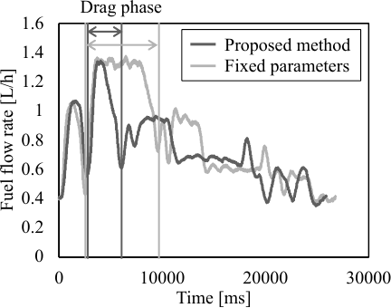
Fig. 14. Fuel flow rate in the field experiments (soft soil). In the dragging phase, the proposed method shortened the operation time compared to the fixed parameters, resulting in a significant reduction in fuel consumption.
Acknowledgments
We would like to thank Editage (www.editage.jp) for English language editing.
- [1] B. Filipe, J. Woetzel, and J. Mischke, “Reinventing Construction: A Route of Higher Productivity,” McKinsey Global Institute, 2017.
- [2] T. Hashimoto, M. Yamada, G. Yamauchi, Y. Nitta, and S. Yuta, “Proposal for Automation System Diagram and Automation Levels for Earthmoving Machinery,” Proc. of the 37th Int. Symposium on Automation and Robotics in Construction (ISARC 2020), pp. 347-352, 2020. https://doi.org/10.22260/ISARC2020/0050
- [3] A. Stentz, J. Bares, S. Singh, and P. Rowe, “A Robotic Excavator for Autonomous Truck Loading,” Autonomous Robots, Vol.7, pp. 175-186, 1999. https://doi.org/10.1023/A:1008914201877
- [4] Y. Yang, L. Zhang, X. Cheng, J. Pan, and R. Yang, “Compact Reachability Map for Excavator Motion Planning,” Proc. of the 2019 IEEE/RSJ Int. Conf. on Intelligent Robots and Systems (IROS), pp. 2308-2313, 2019. https://doi.org/10.1109/IROS40897.2019.8968050
- [5] S. Yoo, C.-G. Parks, S. H. You, and B. Lim, “A Dynamics-based Optimal Trajectory Generation for Controlling an Automated Excavator,” Proc. of the Institution of Mechanical Engineers, Part C: J. of Mechanical Engineering Science, Vol.224, Issue 10, pp. 2109-2119, 2010. https://doi.org/10.1243/09544062JMES2032
- [6] H. Yamamoto, M. Moteki, H. Shao, K. Ootuki, Y. Yanagisawa, Y. Sakaida, A. Nozue, T. Yamaguchi, and S. Yuta, “Development of the Autonomous Hydraulic Excavator Prototype Using 3-D Information for Motion Planning and Control,” Proc. of the 2010 IEEE/SICE Int. Symposium on System Integration, pp. 49-54, 2010. https://doi.org/10.1109/SII.2010.5708300
- [7] R. J. Sandzimier and H. H. Asada, “A Data-Driven Approach to Prediction and Optimal Bucket-Filling Control for Autonomous Excavators,” IEEE Robotics and Automation Letters, Vol.5, No.2, pp. 2682-2689, 2020. https://doi.org/10.1109/LRA.2020.2969944
- [8] Y. B. Kim, J. Ha, H. Kang, P. Y. Kim, J. Park, and F. C. Park, “Dynamically Optimal Trajectories for Earthmoving Excavators,” Automation in Construction, Vol.35, pp. 568-578, 2013. https://doi.org/10.1016/j.autcon.2013.01.007
- [9] S. Lee, D. Hong, H. Park, and J. Bae, “Optimal Path Generation for Excavator with Neural Networks Based Soil Models,” Proc. of the 2008 IEEE Int. Conf. on Multisensor Fusion and Integration for Intelligent Systems, pp. 632-637, 2008. https://doi.org/10.1109/MFI.2008.4648015
- [10] A. R. Reece, “Paper 2: The Fundamental Equation of Earth-Moving Mechanics,” Proc. of the Institution of Mechanical Engineers, Vol.179, Issue 6, pp. 16-22, 1964. https://doi.org/10.1243/PIME_CONF_1964_179_134_02
- [11] O. Luengo, S. Singh, and H. Cannon, “Modeling and Identification of Soil-tool Interaction in Automated Excavation,” Proc. of the 1998 IEEE/RSJ Int. Conf. on Intelligent Robots and Systems, pp. 1900-1906, 1998. https://doi.org/10.1109/IROS.1998.724873
- [12] O. M. U. Eraliev, K.-H. Lee, D.-Y. Shin, and C.-H. Lee, “Sensing, perception, decision, planning and action of autonomous excavators,” Automation in Construction, Vol.141, Article No.104428, 2022. https://doi.org/10.1016/j.autcon.2022.104428
- [13] C. Henderson, A. Levett, and D. Lisle, “The Effects of Soil Water Content and Bulk Density on the Compactibility and Soil Penetration Resistance of Some Western Australian Sandy Soils,” Australian J. of Soil Research, Vol.26, Issue 2, pp. 391-400, 1988. https://doi.org/10.1071/SR9880391
- [14] R. Horn, T. Way, and J. Rostek, “Effect of Repeated Tractor Wheeling on Stress/strain Properties and Consequences on Physical Properties in Structured Arable Soils,” Soil & Tillage Research, Vol.73, Nos.1-2, pp. 101-106, 2003. https://doi.org/10.1016/S0167-1987(03)00103-X
- [15] A. A. G. Al-shammary, A. Z. Kouzani, A. Kaynak, S. Y. Khoo, M. Norton, and W. Gates, “Soil Bulk Density Estimation Methods: A Review,” Pedosphere, Vol.28, Issue 4, pp. 581-596, 2018. https://doi.org/10.1016/S1002-0160(18)60034-7
- [16] A. Nelson, “Dictionary of Mining,” George Newnes, 1965.
- [17] A. Heit, “An Investigation into the Parameters That Affect the Swell Factor Used in Volume and Design Calculations at Callide Open Cut Coal Mine,” Ph.D. Thesis, University of Southern Queensland, 2011.
- [18] C. Wang and Y. K. Cho, “Smart Scanning and Near Real-time 3D Surface Modeling of Dynamic Construction Equipment from a Point Cloud,” Automation in Construction, Vol.49, Part B, pp. 239-249, 2015. https://doi.org/10.1016/j.autcon.2014.06.003
- [19] J. Yang, M.-W. Park, P. A. Vela, and M. Golparvar-Fard, “Construction Performance Monitoring via Still Images, Time-lapse Photos, and Video Streams: Now, Tomorrow, and the Future,” Advanced Engineering Informatics, Vol.29, Issue 2, pp. 211-224, 2015. https://doi.org/10.1016/j.aei.2015.01.011
- [20] C. Yuan, S. Li, and H. Cai, “Vision-Based Excavator Detection and Tracking Using Hybrid Kinematic Shapes and Key Nodes,” J. of Computing in Civil Engineering, Vol.31, Issue 1, Article No.04016038, 2016. https://doi.org/10.1061/(ASCE)CP.1943-5487.0000602
- [21] Y. Sakaida, D. Chugo, H. Yamamoto, and H. Asama, “The Analysis of Excavator Operation by Skillful Operator – Extraction of Common Skills –,” Proc. of the SICE Annual Conf., pp. 538-542, 2008. https://doi.org/10.1109/SICE.2008.4654714
- [22] F. E. Sotiropoulos and H. H. Asada, “A Model-Free Extremum-Seeking Approach to Autonomous Excavator Control Based on Output Power Maximization,” IEEE Robotics and Automation Letters, Vol.4, Issue 2, pp. 1005-1012, 2019. https://doi.org/10.1109/LRA.2019.2893690
- [23] J. H. Holland, “Adaptation in Natural and Artificial Systems: An Introductory Analysis with Applications to Biology, Control, and Artificial Intelligence,” The University of Michigan Press, 1975.
- [24] D. Holz, T. Beer, and T. W. Kuhlen, “Soil Deformation Models for Real-Time Simulation: A Hybrid Approach,” Proc. of Workshop in Virtual Reality Interactions and Physical Simulations (VRIPHYS2009), 2009. https://doi.org/10.2312/PE/vriphys/vriphys09/021-030
- [a] ROS – Robot Operating System. https://www.ros.org [Accessed May 2, 2025]
This article is published under a Creative Commons Attribution-NoDerivatives 4.0 Internationa License.