Ridge-Structure-Based Crop Classification for Small UGV and Derived Detection Framework

Yusuke Iuchi; Soki Nishiwaki; Fan Yi; Takuma Shoji; Ahmad Aizad Bin Azam; Takanori Emaru

doi:10.20965/jrm.2026.p0658

single-rb.php

« previous

JRM Vol.38 No.2 pp. 658-671

(2026)

doi: 10.20965/jrm.2026.p0658

Paper:

Views over last 60 days: 5

Ridge-Structure-Based Crop Classification for Small UGV and Derived Detection Framework

Yusuke Iuchi, Soki Nishiwaki, Fan Yi, Takuma Shoji, Ahmad Aizad Bin Azam, and Takanori Emaru

Hokkaido University
Kita 13, Nishi 8, Kita-ku, Sapporo, Hokkaido 060-8628, Japan

Received:

July 2, 2025

Accepted:

October 28, 2025

Published:

April 20, 2026

Keywords:

crop and weed classification, crop detection, precision agriculture

Abstract

In crop detection, ridge structures provide crucial cues for classifying crops and weeds. However, it is difficult to obtain ridge structures for unmanned ground vehicles which can capture images only within a narrow field of view. This study proposes a lightweight algorithm that enables a model to implicitly infer the ridge structure from plant-to-plant spatial relationships and sizes. An object detector first detects each plant. The resulting bounding boxes are treated as pairwise features in the nodes. Metainformation indicating whether two nodes share the same ID is combined with their geometric relationships and encoded as edge features. A graph attention network addresses these relationships to infer and propagate ridge-aware regularities. By understanding the structure only from object relationships, the method compensates for the information lost to the limited field of view without any explicit edge structure input. In the experiments wherein we deliberately introduced a domain shift between the training/validation sets and test set, the proposed method increased the baseline mAP₅₀ from 30.6% to 44.4%. This amounts to an increase of up to 13.8 percentage points. In addition, the proposed method requires only approximately 10 ms/frame on a Jetson AGX Orin to classify plants. This method acquires ridge structures internally without relying on external sensors or hand-tuned thresholds. Thus, it displays potential for in-field agricultural applications such as autonomous weeding.

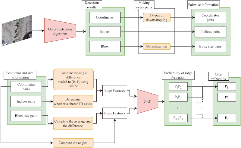
Overview of the proposed framework

Close full text

Cite this article as:

Y. Iuchi, S. Nishiwaki, F. Yi, T. Shoji, A. Azam, and T. Emaru, “Ridge-Structure-Based Crop Classification for Small UGV and Derived Detection Framework,” J. Robot. Mechatron., Vol.38 No.2, pp. 658-671, 2026.

Data files:

1. Introduction

With the global uncertainty over food supply driven by the population growth and climate change, the Food and Agriculture Organization of the United Nations emphasizes that automation can simultaneously improve resource efficiency and alleviate agricultural labor shortages ^a. Smart agriculture technologies that combine robotics with information and communications technology enable small-scale farmers to stabilize the product quality while cutting costs. Japan confronts a similar need because its agricultural workforce is reducing as a result of its aging society ^b. According to these recent trends, the interest in and adoption of IoT- and AI-enabled smart agriculture is increasing ^1,2,3.

Autonomous physical weed control is in high demand because of the increasing requirements to reduce the use of chemical pesticides and regulatory constraints on pesticide application in the production of medicinal crops. Manual intra-row weeding is physically demanding. This hinders the reduction of labor inputs and stabilization of yields. To resolve this problem, autonomous mobile robots capable of performing instance-level field management are essential in conjunction with high-precision crop and weed recognition technologies that play a central role in these systems.

In many ridge-based crop rows, such as soybean and maize, farmers typically perform a hilling operation. Herein, soil is piled around the base of the stems once the plants have grown to the point where the leaves of neighboring individuals start to overlap. After this stage, the crop canopy suppresses weed growth and intra-row weeds are less likely to outcompete the crops. Therefore, the frequency and intensity of manual or robotic weeding can be reduced. Consequently, regular weeding operations are particularly important, and individual plants remain clearly separated. Therefore, in this study, we focus on this early growth stage with separable individuals. And we assume that the proposed method can be deployed under such field conditions.

1.1. Background

Robust image-based crop/weed classifiers and detection methods are required to develop robotic weeding systems for these field conditions. However, image-based crop/weed classifiers generalize ineffectively because (i) the cultivar variety and illumination differences alter the appearance, and (ii) agricultural big data vary widely in purpose and acquisition procedures, thereby limiting the consistency of both quality and format ⁴. Although agricultural datasets such as DeepWeeds ⁵ and CropAndWeed ⁶ are publicly available and the number of such datasets has been increasing gradually, it is still infeasible to include all the species and growth conditions observed on real farms. Fig. 1 compares images of the same soybean cultivar captured from different locations and seasons. Even within the same cultivar, the plants differed in appearance. Similarly, weed types can differ across fields. Consequently, a detection model trained on data from a single farm frequently fails to generalize when deployed in fields that differ in cultivar, growth stage, or environmental condition.

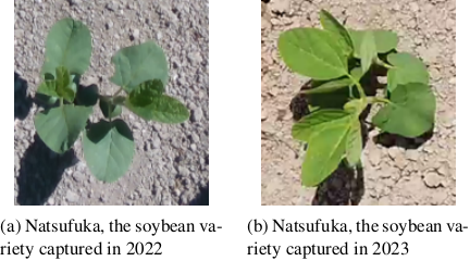
Fig. 1. Two images of soybeans recorded in different years captured by the authors.

On farms where a domain shift of visual features occurs frequently, several studies have detected crops and weeds by utilizing structural features, particularly general ridge patterns between crop rows. The periodic spacing of ridges provides a geometric prior that indicates where crop rows should appear, suppresses background clutter, and straightforwardly isolates weeds between ridges. Recent studies have utilized explicit 3-D ridge geometry or the linear arrangement of crops to enhance plant detection ^7,8,9,10. By incorporating geometric cues that conventional pixel-level detectors cannot capture, these methods enhance the detection accuracy.

However, most approaches assume the availability of dense depth maps or wide-area imagery to capture the linear arrangement of crops. In addition, these occasionally rely on hand-tuned pre-processing thresholds. Consequently, existing approaches fail when ridges are flat or when the camera captures only a narrow area of the field, which is typical for sensors mounted on unmanned ground vehicles (UGVs) in agricultural fields. These limitations hinder the adoption of ridge-aware detection methods for UGVs. Thus, the development of crop and weed detection methods that can be generalized across farms for small robots remains a challenge.

To overcome these limitations, we propose a novel method that learns crop-row structures from limited areas using graph neural networks ¹¹ and graph attention networks (GAT) ¹² without hand-tuned thresholds. By integrating our method with convolutional neural network (CNN)-based object detectors, we achieve higher detection accuracy than conventional CNN-based methods on a domain-shifted dataset.

This study extends the crop classification method by utilizing the ridge structures proposed by the authors ¹³. Although our earlier Transformer-based ridge-aware classifier achieved an accuracy comparable to that of previous crop detection methods, its $O(N^{4})$ complexity made it impractical for edge devices when processing images containing many plants. Moreover, this method uses plant identifiers as features. However, the identifiers are simply assigned in the detection order. As a result, when the number of detected objects differs between frames, previously unobserved IDs can originate. This, in turn, degrades accuracy. To address these problems, this study re-implements this concept in a GAT framework. This reduces the complexity to $O(N^{2})$.

1.2. Related Works

Before deep learning was introduced, crop-weed recognition relied on discriminant analysis ¹⁴, Bayesian decision theory ¹⁵, Otsu’s binarization ¹⁶, and support vector machine (SVM) ¹⁷. Since 2015, convolutional and Transformer-based detectors such as YOLO ^c, the recurrent convolutional neural network (RCNN) family ^18,19,20, and DETR ²¹ have been widely used. Nonetheless, they continue to display domain shift problems.

Sunil et al. ²² conducted accuracy evaluations using detectors such as YOLO and customized architectures. They constructed four crop and weed datasets at three sites over multiple years. Moreover, they performed detection experiments on each individual dataset as well as on a combined dataset. A few datasets achieved mean average precision values at 0.5 IoU above 0.8 for all the models. However, the data collected at Carrington Farm in 2022 showed a decrease in $\mathrm{mAP}_{50}$, with the values ranging from 0.412 to 0.627 for the identical model architectures. The study reported that this phenomenon was caused by the limited size and variation of the datasets, which did not replicate real-field conditions. These observations indicate that on farms with substantially different environments, it is difficult to construct a dataset with a universally applicable feature distribution. This may degrade the generalization performance of detection models.

To improve the accuracy of crop and weed detection on farms, several studies leveraged the ubiquitous ridge structures observed in row-crop agriculture. These provide commonly available geometric information and enhance the crop detection accuracy ^8,7,9,10. Ota et al. ⁷ used depth information with Otsu thresholding and Canny edge detection to identify ridge rows. They then applied $K$-means clustering to detect crops and weeds. Ota’s method achieved an accuracy higher than those of classical methods such as SVM. Although detecting ridge rows from three-dimensional structures is effective on certain farms, it cannot be applied to farms with flat ridges.

Pérez-Ortiz et al. ⁸ used the excess green index (ExG) and Otsu’s binarization in 2016 to separate vegetation from nonvegetation. They then classified crops and weeds by SVM by employing features such as ExG statistics and distances to ridges obtained by the Hough transform. They achieved an accuracy of over 90%. Crop row detection using the Hough transform (which utilizes the ridge structure) is still combined with deep neural networks. De Marinis et al. ⁹ applied classical binarization to aerial images captured by unmanned aerial vehicles (UAVs), detected crop rows using the Hough transform, and attached pseudo-supervisory labels to train a lightweight CNN. Their proposed method attained an F1 score of approximately 0.75. They achieved both substantial reduction in annotation effort and higher detection accuracy by utilizing ridge-structure information. However, the Hough-transform-based ridge-row detection determines the line structures by thresholding. Although it can be used in applications with a wide field of view, such as UAVs, its application remains challenging when a wide field of view is difficult to secure, as with UGVs.

Osco et al. ¹⁰ proposed a method that detects crop rows and counts the number of plants within each row by incrementally updating confidence maps for crop rows and points with a CNN applied to UAV-captured farmland images, while sharing the features of crop rows and points in each stage. Their approach achieved a mean absolute error of 1.409 for citrus count. However, because the method was validated on wide-area images, the detection of crop rows is likely to be unstable in narrow-field images.

Figure 2 shows images for a typical UGV imaging range. Wherein classical binarization, the Hough transform, and ridge-line detection based on ExG centroid positions were applied. Although the Hough transform threshold was lowered sufficiently to detect short segments on the leaves, the scattered arrangement of plants prevented the formation of clear straight ridge lines. In addition, even when centroid positions are used, the detected ridge line can be shifted owing to the weed distribution. Therefore, for ground robots with narrow fields of view, such as UGVs, the assumption of straight-line detection is occasionally difficult.

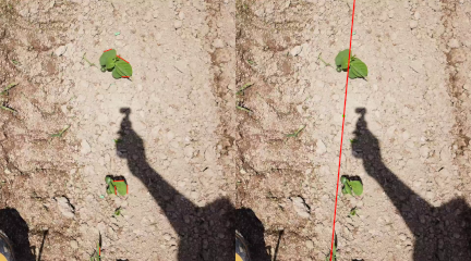
Fig. 2. Examples of straight-line detection performed on binary images generated with the ExG index and Otsu’s thresholding. (Left) The short red lines are detection results obtained using the Hough transform. (Right) The long red line is the detection result obtained using the centroid method.

1.3. Contributions

In UGVs with inherently narrow fields of view, the spacing between individual plants generally degrades the estimation of crop row structure. This issue originates from the earliest germination stage until the canopies of neighboring plants begin to overlap. To address this problem, we proposed an algorithm that infers ridge structures based on interplant spatial relationships. Combined with CNN- or Transformer-based plant detectors, the proposed module classifies plants into crops or weeds based only on the relationship between their locations, without class-specific visual features.

We developed a classification framework that utilizes the inferred ridge structures obtained from plant size and alignment as discriminative features even in situations where straight ridge lines are not explicitly present.
Through a quantitative comparison with existing crop-detection methods, we evaluated the importance of modeling ridge structures for crop detection even in farms where ridges are absent (e.g., flat-bed fields) and on robotic platforms for which crop-row detection is challenging (e.g., small UGVs).

2. Methodologies

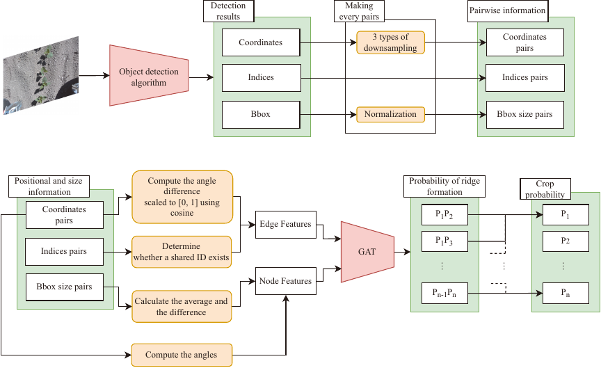
Fig. 3. The diagram illustrates the object detection process and the detailed architecture in the proposed method. The rectangles with sharp right angles represent data or numeric values. The orange rectangles with rounded corners represent operations performed on that data. The red shapes represent the entire network architecture.

This section outlines the proposed method. It accepts the detected plant location and size information as inputs to the GAT ¹². The proposed system adopts a two-stage processing pipeline: (1) individual plants are detected and (2) these are classified into crop or non-crop categories. An overview of the entire system is shown in Fig. 3.

2.1. Preprocess

Initially, we trained the detector using a conventional object-detection algorithm based on both CNN- and Transformer-based detectors. The center coordinates and temporary IDs were obtained for each bounding box extracted from the target image using this detector. To reduce the dependence of the bounding-box center coordinates on the image resolution, we recomputed the centers in a three-stage downsampled coordinate system, as defined in Eqs. $\eqref{eq:low_center}$ and $\eqref{eq:low_point}$. Accordingly, the network maintained three resolution-aware coordinate sets for each object. In this study, the downsampled resolutions were set such that the shorter side lengths were 20, 80, and 320 pixels. The use of multiresolution coordinate systems enables the model to capture positional information ranging from fine-grained to global spatial relationships while maintaining a low feature dimensionality.

\begin{align} \Delta_{x}^{(r)} &= \frac{W}{r}, \quad \Delta_{y}^{(r)} = \frac{H}{r}, \tag{1a}\label{eq:low_center} \\ \end{align}

\begin{align} \boldsymbol{d}_{n}^{(r)} &= \left(\left\lfloor \dfrac{c_{x}^{(n)}}{\Delta_{x}^{(r)}}\right\rfloor,\, \left\lfloor \dfrac{c_{y}^{(n)}}{\Delta_{y}^{(r)}}\right\rfloor \right) \in \mathbb{Z}^{2}, \tag{1b}\label{eq:low_point} \end{align}

where $(H, W)$ denotes the image resolution, $r \in \{20, 80, 320\}$ is the division factor, and $\boldsymbol{d}_{n}^{(r)}$ represents the coarse-grained pixel coordinate of an object $n$. $\boldsymbol{c}_n$ indicates the center coordinates of the bounding boxes.

Next, for each pair of plants, we computed the orientation of the vector connecting the centers of their respective bounding boxes, as shown in Eqs. $\eqref{eq:pair_vec}$–$\eqref{eq:theta}$. We then generated a node for each unique pair of detected objects, i.e., for each unordered ID combination $(i, j)$. Each bounding box was considered as a node attribute. Meanwhile, the angular differences between the vectors and the corresponding ID pair were employed as edge attributes to represent the relationships between nodes.

\begin{align} \tilde{\boldsymbol{v}}^{(r)}_{ij} &= \boldsymbol{d}^{(r)}_{j} - \boldsymbol{d}^{(r)}_{i} \in \mathbb{Z}^{2}, \tag{2a}\label{eq:pair_vec}\\ \end{align}

\begin{align} \boldsymbol{v}^{(r)}_{ij} &= \left\{ \begin{aligned} &\tilde{\boldsymbol{v}}^{(r)}_{ij}, &&\mbox{if $\tilde{v}^{(r)}_{ij,y} \ge 0$}, \\ &- \tilde{\boldsymbol{v}}^{(r)}_{ij}, &&\text{otherwise}, \end{aligned}\right. \tag{2b}\label{eq:pair-diff} \\ \end{align}

\begin{align} \theta_{ij}^{(r)} &= \arccos \left( \frac{\boldsymbol{v}_{ij}^{(r)} \cdot \hat{\boldsymbol{u}}} {\left\|\boldsymbol{v}_{ij}^{(r)}\right\|} \right), \tag{2c}\label{eq:theta} \end{align}

where $\boldsymbol{v}_{ij}^{(r)}$ is a vector that locates the center positions between plants $i$ and $j$. The $y$ components were maintained positive. $\theta_{ij}^{(r)}$ denotes the orientation of $\boldsymbol{v}_{ij}^{(r)}$. $\hat{\boldsymbol{u}}$ is the unit vector along the positive $x$-axis of the image.

2.2. Edge Features

The number of edges in a fully connected graph grows quadratically $O(N^{2})$. Therefore, we pruned the edges to improve the computational efficiency while maintaining the local structure. For each node that encodes pairwise information, we construct an adjacency matrix by applying the K-NN criterion ²³. We retained the $K$ edges with the smallest angular differences. Crop rows are typically planted in nearly straight lines. Consequently, if the vectors connecting the two plant pairs are almost parallel, the corresponding plants are likely to lie on the same ridge. Therefore, we first discarded edges with larger angular differences. This enabled the network to encode the ridge structure.

As shown in Eq. (3), the edge feature is the cosine of the angular difference for each pair, computed in three distinct coordinate systems. In addition to this parallelism, we attached a binary attribute indicating whether two connected nodes share an ID. A one-bit flag indicating whether two nodes share at least one ID was appended to the tail of the edge feature vector. Consequently, each edge serves as a multifaceted descriptor that jointly encodes geometric relationships and initial labels.

\begin{align} \varphi_{kl}^{(r)} &= \theta_{k}^{(r)} - \theta_{l}^{(r)}, \tag{3a}\label{eq:phi} \\ \end{align}

\begin{align} \rho_{kl}^{(r)} &= \left|\cos\varphi_{kl}^{(r)}\right|, \tag{3b}\\ \end{align}

\begin{align} \delta_{kl} &= \begin{cases} 1, &\mbox{if the pair shares the same ID},\\ 0, &\mbox{otherwise}, \end{cases}\tag{3c} \\ \end{align}

\begin{align} \boldsymbol{e}_{kl} &= \left[\rho_{kl}^{(r)},\delta_{kl}\right] \in \mathbb{R}^{4}, \tag{3d} \end{align}

where $k$ denotes the index of a node, and $l$ represents one of its neighboring nodes. $\theta_{k}^{(r)}$ and $\theta_{l}^{(r)}$ refer to the orientation values of nodes $k$ and $l$, respectively. $\rho_{kl}$ measures the degree of parallelism between the two nodes. $\delta_{kl}$ is a binary indicator specifying whether these share an identifier, and $\boldsymbol{e}_{kl}$ denotes the corresponding edge feature.

2.3. Node Features

On the node side, we first mitigated the sample-specific scale bias by adding an $\varepsilon$-stability term to the width and height of each bounding box (considering the logarithm) and then subtracting the average log-diagonal length. This is formalized in Eq. $\eqref{eq:antei}$. From these stabilized values, for each pairwise node, we computed the mean and difference between the two bounding boxes (see Eq. $\eqref{eq:node_f}$. This difference captured the size discrepancy between the two boxes. Meanwhile, the mean was used as the reference scale when comparing this pair with the other pairs. To further stabilize the gradient computation, the mean was converted into $\tilde{m}_{ij}$ by subtracting the minimum mean value, ${\min m}$, within the same graph, as described by Eq. $\eqref{eq:node_norm}$. Finally, concatenating these two vectors yielded the node feature $\operatorname{box{\_}feat}_{ij}$, as expressed in Eq. $\eqref{eq:box_feat}$.

\begin{align} u_{i} &= \log\bigl(s_{i} + \varepsilon\bigr), \tag{4a}\label{eq:antei} \\ \end{align}

\begin{align} d_{ij} &= \left|u_{i} - u_{j}\right|, \quad m_{ij} = \dfrac{u_{i} + u_{j}}{2}, \tag{4b}\label{eq:node_f} \\ \end{align}

\begin{align} \tilde{m}_{ij} &= m_{ij} - \min m, \tag{4c}\label{eq:node_norm} \\ \end{align}

\begin{align} \operatorname{box{\_}feat}_{ij} &= \bigl[\tilde{m}_{ij}, d_{ij}\bigr] \in \mathbb{R}^{2}, \tag{4d}\label{eq:box_feat} \end{align}

where $s_{i}$ denotes the area of the bounding box with ID $i$, and $\varepsilon$ represents a stabilization term. The logarithms of these quantities are denoted as $u_{i}$. $d_{ij}$ and $m_{ij}$ represent the difference and mean, respectively, of the areas of the $i$-th and $j$-th bounding boxes. The adjusted mean value $\tilde{m}_{ij}$ was obtained by subtracting the minimum value ${\min m}$ from the same graph as $m_{ij}$.

The orientation $\theta_{ij}^{(r)}$ in Eq. $\eqref{eq:theta}$ is used to calculate the directional agnostic angle feature $\operatorname{angle{\_}feat}_{ij}$ as shown in Eq. $\eqref{eq:angle_feat}$. Finally, the variable concatenating the angle feature $\operatorname{angle{\_}feat}_{ij}$ with $\operatorname{box{\_}feat}_{ij}$ is expressed by Eq. $\eqref{eq:nodefeat_0}$. $x_{k}^{(0)}$ is then projected onto a higher dimensional space via a linear layer and normalized as an input to the GAT.

\begin{align} &\operatorname{angle{\_}feat}_{ij} \notag \\ &\hspace{1.5em} = \left( \cos\theta_{ij}^{(1)}, \dots, \cos\theta_{ij}^{(r)}, \sin\theta_{ij}^{(1)}, \dots, \sin\theta_{ij}^{(r)} \right) \in \mathbb{R}^{2r}, \tag{5a}\label{eq:angle_feat} \\ \end{align}

\begin{align} &\boldsymbol{x}_{k}^{(0)} = \boldsymbol{x}_{ij} = \bigl[\operatorname{box{\_}feat}_{ij}, \operatorname{angle{\_}feat}_{ij}\bigr], \tag{5b}\label{eq:nodefeat_0} \end{align}

where $\boldsymbol{x}_{k}^{(0)}$ represents the initial node feature of a given node. $\boldsymbol{x}_{ij}$ is the node feature computed from the bounding-box information corresponding to ID $(i,j)$.

2.4. GAT

First, a graph represented by node features, edge features, and an adjacency matrix is fed into a GAT composed of two consecutive GATConv layers. GAT extends the graph convolutional network ¹¹, which aggregates neighboring node features via convolutions that respect the graph structure by incorporating an attention mechanism ²⁴ that learns the attention coefficients between adjacent nodes.

Each GAT layer comprises a GATConv operation (Eqs. $\eqref{eq:gatconv1}$–$\eqref{eq:headcat}$, followed by layer normalization (LN) ²⁵ and exponential linear unit (ELU) activation ²⁶. Within the two-layer sequence, the first GATConv layer concatenates its attention heads, as shown in Eq. $\eqref{eq:headcat}$, whereas the second method aggregates these without concatenation.

\begin{align} \tilde{\boldsymbol{h}}_{k}^{(\ell,h)} &= \boldsymbol{W}^{(\ell,h)} \boldsymbol{x}_{k}^{(\ell-1)}, \quad \tilde{\boldsymbol{e}}_{kl}^{(\ell)} = \boldsymbol{W}_{e}^{(\ell)} \boldsymbol{e}_{kl}, \tag{6a}\label{eq:gatconv1} \\ \end{align}

\begin{align} e_{kl}^{(\ell,h)} &= \operatorname{LeakyReLU}\left( \boldsymbol{a}^{(\ell,h) \top} \left[ \tilde{\boldsymbol{h}}_{k}^{(\ell,h)} \left\| \tilde{\boldsymbol{h}}_{l}^{(\ell,h)} \right\| \tilde{\boldsymbol{e}}_{kl}^{(\ell)} \right] \right), \tag{6b}\label{eq:cat} \\ \end{align}

\begin{align} \alpha_{kl}^{(\ell,h)} &= \frac{\exp \left(e_{kl}^{(\ell,h)}\right)} {\displaystyle \sum_{t \in \mathcal{N}(k)\cup\{k\}} \exp \left(e_{kt}^{(\ell,h)}\right)}, \tag{6c}\\ \end{align}

\begin{align} \boldsymbol{x}_{k}^{(\ell,h)} &= \sigma \left( \sum_{l \in \mathcal{N}(k) \cup \{k\}} \alpha_{kl}^{(\ell,h)} \tilde{\boldsymbol{h}}_{l}^{(\ell,h)} \right), \tag{6d}\\ \end{align}

\begin{align} \boldsymbol{x}_{k}^{(\ell)} &= \left\{\begin{aligned} &\displaystyle \bigoplus_{h=1}^{H} \boldsymbol{x}_{k}^{(\ell,h)}, &&\mbox{$\textrm{concat} = \textrm{True}$}, \\ &\displaystyle \frac{1}{H} \sum_{h=1}^{H} \boldsymbol{x}_{k}^{(\ell,h)}, &&\mbox{$\textrm{concat} = \textrm{False}$}. \end{aligned} \right. \tag{6e}\label{eq:headcat} \end{align}

Because each sample originates from a different farm or crop and contains a variable number of nodes, batch normalization (BN) ²⁷ yields unstable statistics. LN (which is independent of batch statistics) was adopted. The ELU was selected to prevent vanishing gradients in the negative region, and thus retain informative signals from the nodes of different classes.

The outputs of the second GAT layer were passed through a linear layer that mapped the features of each adjacent node pair to a scalar logit, thus representing the likelihood that the pair belonged to the same crop row. This logit was converted into a probability using the sigmoid function as in Eq. $\eqref{eq:logit}$. The training employed binary cross-entropy loss (BCELoss). Herein, the node label was set to one when the node contained only crop points and to zero when weed points were present.

\begin{equation} p_{k} = \sigma \left(\boldsymbol{w}_{o}^{\top} \boldsymbol{x}_{k}^{(L)} + b_{o}\right) \tag{7}\label{eq:logit} \end{equation}

In the above equations, $\ell$ denotes the layer index and $h$ the head index. $\boldsymbol{x}_{k}^{(\ell-1)}$ is the node embedding from the previous layer, and $\boldsymbol{W}$ is a linear transformation matrix. $\boldsymbol{a}^{(\ell,h)}$ is the attention weight vector for head $h$, and $\alpha_{kl}$ is the attention coefficient. $\mathcal{N}(k)$ denotes the set of nodes adjacent to node $k$, and $\boldsymbol{x}_{k}^{(\ell,h)}$ is the output of head $h$. The GATConv operation includes self-looping. $\boldsymbol{w}_{o}^{\top}$ and $b_{o}$ are the output-layer weight vector and bias, respectively, and $\sigma$ is the sigmoid function. Finally, $p_k$ denotes the probability that node $k$ forms a ridge.

2.5. Pair to ID Classes Conversion

The value obtained for each node probabilistically indicates whether node plants are crops or weeds. This value is computed from the similarity of the bounding box sizes and the parallelism of their relative positions. To propagate the node-level results to the object instances (IDs), we first assigned a score to each ID contained in the nodes classified as Class 1, as expressed in Eq. $\eqref{eq:vote1}$. We summed the scores for each ID as indicated in Eq. $\eqref{eq:vote2}$. If an ID’s aggregated score was higher than 20% of the maximum, the object was classified as a crop. Otherwise, it was considered a weed. Unlike methods that directly infer classes from raw feature vectors, this voting-based approach provides higher robustness against outliers.

\begin{align} \hat{y}_{ik} &= \mathbf{1}\left[p_{k} > \tau\right], \tag{8a}\label{eq:vote1} \\ \end{align}

\begin{align} r_{i} &= \sum_{k=1}^{N-1} \hat{y}_{ik}, \tag{8b}\label{eq:vote2} \end{align}

where $\hat{y}_{ik}$ denotes the score for ID $i$ within node $k$, and $r_i$ represents the total score for ID $i$ across all nodes.

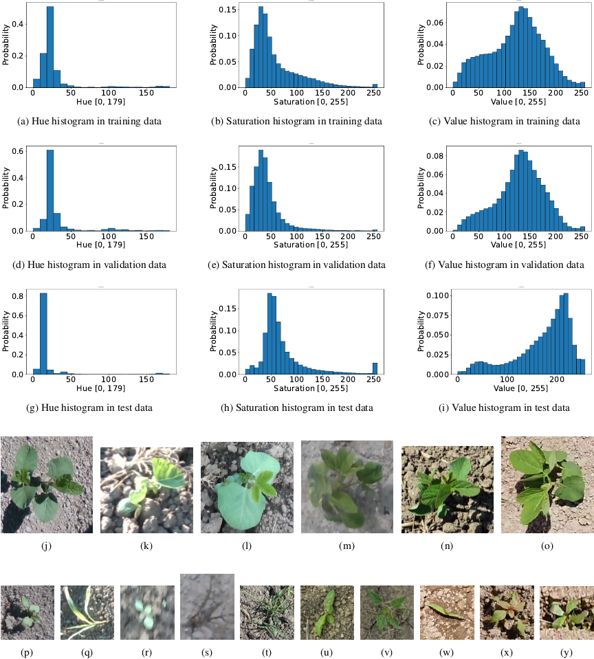
Fig. 4. The statistics figures show color histograms for each dataset in conjunction with representative soybean images. The histograms plot the element values on the horizontal axis and the frequencies on the vertical axis. The plant images are actual images of the dataset. The training and validation sets consist of data captured under the conditions in images (j)–(n). The test set comprises only data captured in the environment of image (o). Images (j), (k), (l), and (o) depict the same cultivar. In particular, images (j) and (o) were extracted from the same field. The only difference is the shooting year. Image (n) is a cropped example extracted from ave-0596-0007.jpg in the CropAndWeed dataset ⁶. Additionally, images (p)–(v) illustrate examples of weeds included in the training set, whereas images (w)–(y) illustrate those included in the test set. Among these weeds, (t), (u), and (v) correspond to ave-0313-0008.jpg, ave-0325-0007.jpg, and vwg-0519-0007.jpg in the CropAndWeed dataset, respectively. All the other weed images were photographed by the authors in Hokkaido.

3. Experimentations

We evaluated our ridge-aware re-classification pipeline on soybean-weed images collected in Hokkaido (2021–2024) and on the soybean subset of CropAndWeed ⁶. The split consisted of 3968 training, 589 validation, and 495 test images. The test data was captured a year after the training and validation data were captured to emulate the real-world domain shift.

Figure 4 shows representative images from the datasets and their HSV histograms. It highlights the color shift between the training and validation domains and the 2024 test domain.

3.1. Model and Training Setup

As baselines, we trained Cascade R-CNN ²⁰, RetinaNet ²⁸, YOLOv8-l ^c, YOLOv12 [29, d], and DINO ³⁰ starting from publicly released COCO ³¹ weights. This was performed so that each architectural paradigm (two-stage, dense one-stage, anchor-free, and Transformer-based) was represented. The performance is reported in terms of the mean average precision at 0.5 IoU ($\mathrm{mAP}_{50}$), $\mathrm{mAP}_{50:95}$, and class-wise AP. Additionally, the inference speed was measured during the test. the non-maximum suppression (NMS) times were excluded from the inference time.

All the detectors were optimized for 100 epochs using AdamW. An effective batch size of 16 was obtained via gradient accumulation. A base learning rate (lr) of $2.5 \times 10^{-4}$ was used. For Transformer base lr was reduced to $1.0 \times 10^{-4}$ to stabilize the training. The training was stopped when the validation mAP failed to improve for 10 consecutive epochs. All the experiments were run on a single Nvidia RTX A6000 ADA. The latency was benchmarked on a Jetson AGX Orin.

A global confidence threshold of 0.25 was applied to each detector. For the CNN-based models, we evaluated two variants: (i) conventional class-dependent NMS and (ii) class-agnostic NMS that maintains the highest-scoring box irrespective of class. The latter variant fed our two-layer GAT, which re-labeled boxes according to the ridge geometry. DINO uses a single box per query. Thus, it bypassed NMS and was passed unaltered to the GAT.

To focus the refinement network mainly on geometry, we trained the GAT only on positional graphs extracted from corn, adlay, pumpkins, and weeds. This is shown in Fig. 5. Soybean data were used only to test the generality of our method and were not used for training. In some datasets, photographs contained only a single crop. In such cases, it is difficult for the proposed method to learn the row structure. Therefore, we did not use those photographs when training our method. Node coordinates were augmented by random border crops and random rotations, so that the model learned relative positions rather than absolute positions.

Furthermore, we compared the inference speed and accuracy of the proposed method with a Transformer-based implementation of the concept proposed in ¹³. The key difference is that the features encoded by the GAT as edge attributes are handled directly within the input at an equal level to that of the bounding box and angle information. The Transformer-based variant is trained using a previously described methodology ¹³. Compared with the observations in ¹³, lowering the threshold of the preceding object-detection algorithm from 0.5 to 0.25 enabled the detection of more crops and weeds. This increased the complexity of the classification task.

3.2. Validation of Graph Construction

The assumptions for the proposed graph construction are as follows:

Consider each detected pair of plants (two instances) as a node.
Encode angular parallelism and size statistics as node and edge features.

To verify the correctness of this construction, we selected (i) images in which the proposed model provided many correct classifications and (ii) images in which the proposed model detected several failures. For each image, we computed summary statistics separately for the crop–crop (cc), crop–weed (cw), and weed–weed (ww) pairs. On the node side, we used the absolute difference between the log-scaled bounding box areas, $d_{ij}$, and adjusted mean $\tilde{m}_{ij}$ as mentioned previously. As an edge feature, we measured the degree of parallelism between two nodes $(k,l)$, $\rho_{kl}$, computed from the orientation differences of the center-to-center vectors in the three downsampled coordinate systems. Because the absolute orientation $\theta_{ij}$ is image-dependent and becomes highly dispersed when aggregated across images and because node-configuration angles can be inferred reasonably from the relative parallelism $\rho$, we do not report $\theta$ in the table.

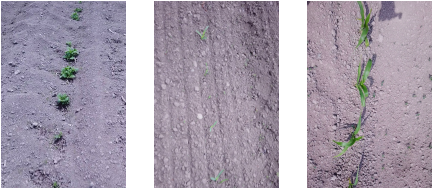
Fig. 5. Examples of the data using in GAT training. The image on the left contains pumpkin plants, the image in the center contains early-stage corn plants, and the image on the right contains mid-stage corn plants. The photographs were captured by the authors in 2023.

Table 1. Accuracy metrics of validation, where class-dep. and class-agn. refer to class-dependent and class-agnostic NMS, respectively.

4. Results

Table 1 presents the detection performance for the validation dataset. Table 2 summarizes the corresponding results for the test dataset. Table 3 compares Transformer-based implementations of the proposed GAT model. The actual detection results are shown in Fig. 6. On the validation dataset, YOLOv8 achieved the best performance, with $\mathrm{mAP} = 0.650$ and $\mathrm{mAP}_{50} = 0.853$. YOLOv12 achieved the second-highest performance, with $\mathrm{mAP} = 0.646$ and $\mathrm{mAP}_{50} = 0.847$. Meanwhile, Cascade R-CNN and RetinaNet remained within the mAP range of 0.542 to 0.545. DINO is the only model that employs a pure Transformer architecture. It yielded a moderate $\mathrm{mAP}$ of 0.615. However this model attained the highest value, $\mathrm{mAP}_{50} = 0.862$. Among all the models, the difference between class-dependent and class-agnostic NMS was less than 0.003. This indicates that the NMS setting had only a marginal impact on the validation setting.

In the test dataset, the ranking varied substantially. DINO achieved the best ranking, $\mathrm{mAP}_{50} = 0.525$, followed by RetinaNet (0.479), Cascade R-CNN (0.460), YOLOv12 (0.356), and YOLOv8 (0.306). After the proposed post-processing was applied, YOLOv8 improved from 0.306 to 0.444 ($+$0.138), YOLOv12 from 0.356 to 0.449 ($+$0.093), Cascade R-CNN from 0.460 to 0.508 ($+$0.048), and RetinaNet from 0.479 to 0.508 ($+$0.029). In particular, the $\mathrm{AP}_{50}$ of the soybean class increased by up to 0.26. In contrast, DINO decreased in $\mathrm{mAP}_{50}$ from 0.525 to 0.448. Compared with the Transformer-based implementation, the overall accuracy reduced.

Table 3. Comparison of accuracy and throughput with the Transformer-based implementation from GAT in the test set. The values in parentheses indicate the difference from GAT.

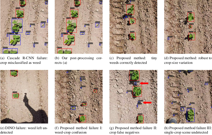
Fig. 6. Qualitative results of crop-weed detection on the field dataset. (a) Cascade R-CNN misclassifies a crop as a weed. (b) Our post-processing corrects the scene in (a). (c) The proposed method correctly detects tiny weeds on the crop row. (d) The method remains robust to moderate crop-size variation. (e) DINO fails to detect weeds whose appearance differs from that of the training set. (f) Failure 1: weeds and crops of similar size are misperceived. (g) Failure 2: a large size disparity causes crop false negatives. (h) Failure 3: single-crop scenes are overlooked owing to row-pair assumption.

Table 4 reports the statistics used for the graph construction. These were computed separately on images dominated by positive vs. negative samples. The annotations mentioned in Table 4 are as follows:

cc denotes a pair of crops.
cw denotes pairs of crops and weeds.
ww denotes a pair of weeds.
cc–cc denotes the edges between the pairs of cc.
The other denotes the other edges.

The edge parallelism $\rho$ is measured per edge from multi-scale directional agreement and then summarized within each image. Meanwhile, node features $\tilde{m}$ (log-scale mean) and $d$ (log-scale difference) summarize the size relationships within node (pair) types.

The parallelism $\rho$ for cc–cc edges is saturated near 1.0 in both the groups. Meanwhile, the others show lower $\rho$. This indicates that the edge definition captures row-wise alignment among crops and does not emphasize mixed/weed relationships. On the node side, the positive cases exhibit larger and more homogeneous crop–crop scales (higher $\tilde{m}$, lower $d$), whereas the negative cases show dispersed crop sizes (lower $\tilde{m}$, higher $d$), in conjunction with noisier layouts. When combined, the proposed node ($\tilde{m}$, $d$) and edge ($\rho$) features induce a coherent graph aligned with field geometry. Thus, this structure weakens in negative cases.

Table 4. Statistics used for graph construction, estimated separately from images dominated by positive and negative samples. Here, cc denotes node pairs comprising two crops, cw denotes crop–weed pairs, and ww denotes weed–weed pairs. cc–cc indicates the edges between two crop-only nodes, and the other node combinations.

5. Discussions

The existing CNN-based and Transformer-based detectors reduced the accuracy in the test sets (Fig. 6(a)). The reduction was largest for weeds. This was because weeds that were not included in the training occupied only a few pixels, and their features were lost straightforwardly in noise after downsampling.

On the test set, class-agnostic NMS had a crop detection accuracy lower than that for class-dependent NMS (${\delta\mathrm{AP}}_{50,\mathrm{soy}} = -3.1$% to $-14.4$%). The redundant crop $+$ weed hypothesis generally received a higher weed score. In practice, this risk mandates a fail-safe rule wherein any dual-label instance is considered a crop.

YOLO was particularly vulnerable: a domain-shifted leaf color or the leaf vein visibility appeared to be distorted by BN statistics. Replacing BN with group normalization or instance normalization could alleviate this effect. However, it is likely to slow the inference because BN folding would be precluded. Integrating the proposed ridge-based postprocessing into YOLOv8 and YOLOv12 reduced the number of false positives in crops. This improved the crop recall and weed precision. Light-weight detectors cannot flexibly extract leaf features. Therefore, adding explicit ridge information produced the largest performance gains.

RetinaNet and Cascade R-CNN (whose heads do not feature BN) showed smaller statistical shifts and, thus, milder degradation. RetinaNet’s dense anchors softened the scale mismatch, whereas Cascade R-CNN’s multi-stage training provided redundancy. These characteristics may have contributed to their higher mAP compared with YOLO in test sets.

Across the CNNs, classifying each detected box with ridge cues produced concurrent gains in weed precision and crop recall. This increased the overall mAP. As shown in Figs. 6(b)–(d), ridge information is color-invariant and species-agnostic. This explains its robustness under a distribution shift.

In our experiments, the Transformer-based DINO preserved the crop mAP between validation and test sets. This suggests that its long-range self-attention may contribute to robustness against such shifts. However, it was slow (0.89 fps on Jetson Orin vs. 10 fps for YOLOv8). DINO relies on the global attention between queries and pixels to detect plants. This resulted in a low sensitivity to small weeds that were not included in training set as shown in Fig. 6(e).

Although the result of DINO showed the best soy detection accuracy in the test set, the accuracy of our method with DINO decreased because the crop growth stages were heterogeneous. As shown in Fig. 6(g), the test images contained soybean plants at both germination and the later stages. Existing networks accurately detect crops at the germination stage because of shape similarity. However, when relative size similarity is lost, the proposed classifier fails. When the shapes match the training set, DINO accurately detects small objects. Therefore, its capability to detect crops smaller than those detected by CNNs resulted in a reduced accuracy after reclassification.

The Transformer-based method proposed previously by the authors failed to achieve a higher accuracy. Unlike the GAT, it considers the sharing of IDs as an internal feature. Within this network, an ID was obtained by embedding the detection order. IDs from approximately 1 to 10 appeared frequently, and the network becomes biased toward those particular IDs. To suppress this effect, in the study ¹³, we fixed an upper bound on the number of plants in an image and randomly remapped the IDs. However, when the upper bound is large, the model cannot learn the relationships for each feasible IDs before the loss function converges. This results in a lower accuracy in this study. On the other hand, the GAT can represent ID sharing directly as an edge feature. It does not confront this problem. In addition, the inference speed was slower than that of the GAT implementation. As mentioned in the Introduction, the computational complexity of a Transformer is $O(N^4)$ with a pairwise node. Therefore, even when classifying an equal number of objects, the Transformer-based implementation ran slower than the GAT. The weed density is likely to increase even further in the field before weeding. Thus, the difference in inference speed widens further.

As illustrated in Fig. 6(f), the proposed method occasionally misidentified the linear pattern of the ridge when the crop positions were sparse and weeds of similar sizes were nearby. Because the classifier relies on relative linearity and size, such errors occur under non-uniform growth conditions. Geometric cues alone cannot differentiate weeds that match the crop size and alignment.

Finally, we analyzed another limitation of this study. The proposed method uses pairwise crop information. Thus, it fails when only one crop appears in the image (Fig. 6(h)). However, during cross-row traversal, retaining the detection information from several previous frames may enable classification even when a single object is visible. The stored information consists of only textual detection results. Therefore, the buffering frames incur a negligible computational overhead.

6. Conclusion

We proposed a lightweight graph attention module that infers ridge geometry from relative crop-weed positions and sizes, and classifies objects using geometry alone, without visual features. It achieved 10 ms/iteration and 13.8% gain in mAP$_{50}$ on a Jetson AGX Orin. Eliminating manual thresholds enables more flexible ridge modeling. This is regarded as a contribution of this study. The module improved the accuracy across diverse CNN-based detectors, thereby demonstrating the practicality of ridge-aware classification using edge devices. Although ridge cues alone fail under growth-stage imbalances, integrating visual features and scaling to large UAV scenes using hierarchical graph methods constitutes a potential future direction. Additionally, in future work, we plan to conduct a large-scale validation to further assess the robustness and generalization.

Appendix A. Detailed Settings of Experiments

In this appendix, we describe the detailed settings of the experiments.

We compared the detection accuracy of baseline object-detection methods with that of our proposed approach. The baseline models were trained with MMDetection ³² and Ultralytics ^c.

The training was conducted using the CropAndWeed dataset ⁶ in conjunction with additional data collected from several farms in Hokkaido. CropAndWeed contains over 7,000 annotated crop-and-weed images. These are further subdivided by growth stage and crop species. To prevent a reduction in accuracy, we retained only images containing soybeans and weeds and discarded those that contained other crops. Supplementary images acquired at the Hokkaido University Experimental Farm were used for the training and validation. All the images were captured in Hokkaido at a height of approximately 80–120 cm above the ground.

The final dataset consists of 3,968 training images, 589 validation images, and 495 test images. To evaluate the detection accuracy under diverse conditions, images were captured using four cameras: Intel RealSense D435, Stereolabs ZED 2 stereo camera, DJI Osmo Pocket, and DJI Osmo Pocket 3. Before the random-resize augmentation, the original image resolutions were $640 \times 480$ and $1920 \times 1080$ pixels. The image resolution of the test set was $960 \times 1080$ pixels.

To accurately assess the generalization capability of both proposed method and baseline networks, the final evaluation was performed on test data that comprised the same soybean cultivar (but were captured in different years) as the training data. Consequently, although the training and validation datasets were collected under identical environmental conditions, the test dataset differed in terms of illumination, crop, and soil conditions. Employing data recorded on different dates for the test and validation sets enabled us to evaluate the robustness of the diverse environments found in real-world farms. For model development, we used images of soybeans captured in Hokkaido from 2021 to 2023 supplemented with the soybean subset of the CropAndWeed dataset for training and validation. The test images were captured in 2024. Portions of the training and validation data included images of the soybean cultivar that appeared in the test set. Except for the CropAndWeed images, all the photographs were captured directly above the ridge lines at an altitude of at most 1 m to evaluate the performance under conditions similar to when the model was mounted on a UGV. Fig. 4 shows color histograms and representative images of each dataset. Although all the images contain both soybean and weed instances, the figure and histograms show that their color distributions differ significantly owing to the differences in lighting conditions and weed composition.

As baseline detectors, we evaluated Cascade R-CNN ²⁰, YOLOv8 ^c, YOLOv12 [29, d], RetinaNet ²⁸, and DINO ³⁰. Because an exhaustive tuning of each model to its optimal performance is impractical, we initialized all the detectors with publicly released weights pretrained on the COCO dataset ³¹ and trained these under common hyperparameter settings. The training was performed on an Nvidia RTX A6000 ADA. The inference measurements were obtained on an Nvidia Jetson AGX Orin. The hyperparameters adopted are listed in Table 5. Following the COCO linear-scaling rule, we used a base learning rate of $2.5 \times 10^{-4}$ and set the backbone learning rate to 0.5 times the base LR. For Transformer-based detectors, the training loss became excessively unstable on background-only image. Therefore, we reduced the learning rate to $1.0 \times 10^{-4}$ and the backbone learning rate to 0.1 times the base LR. All the other settings were identical to those listed in Table 5.

To satisfy the GPU memory budget, we accumulated gradients over microbatches such that the effective batch size was fixed at $B_{\mathrm{eff}} = 16$. During accumulation, no parameters were updated. We applied gradient clipping and performed a single AdamW ³³ update step. Because AdamW was invoked once per effective batch, its momentum estimates, weight decay, and learning-rate schedule were equivalent to those obtained using a real batch of size $B_{\mathrm{eff}}$. Although gradient accumulation introduces additional stochasticity into batch-normalization statistics, other stochastic components such as data augmentation and dropout also contribute to the variation. Because our goal was to compare appearance-driven and structure-driven model architectures, we did not analyze these statistical fluctuations. Transformer-based detectors use layer normalization and were trained with a micro-batch size of one. Therefore, their statistics were independent of the batch size.

By controlling the batch size in this manner, we eliminated it as a confounding variable and could evaluate the architectural generalization under limited computational resources. To accommodate the differences in color histograms and crop sizes among the fields, all the models were trained using horizontal and vertical flipping, random color jitter, and random resizing. At the time of inference the confidence threshold was fixed at 0.25. We applied both the conventional class-specific NMS and a class-agnostic variant in which overlapping boxes were scored jointly across all class probabilities. The box with the highest score was retained. Class-agnostic NMS is desirable for agricultural tasks such as weeding and pesticide spraying because conventional NMS alone cannot sufficiently suppress false weed removal. DINO directly outputs uniquely classified bounding boxes and therefore does not require NMS. The training was stopped early if the detection accuracy failed to improve over 10 consecutive epochs.

To evaluate the importance of understanding ridge structures in small UGVs, we first detected crops and weeds using a previously described algorithm and then re-assigned the classes of the detected plants using the proposed method. The GAT in the proposed framework is not designed to handle cases in which the bounding boxes are spatially identical, i.e., they have equal center, height, and width. Under such circumstances, class-dependent NMS cannot correctly classify objects. Therefore, for the CNN-based detectors, we applied class-agnostic NMS to retain a single bounding box per object before integrating the proposed method. The GAT module is implemented with two layers, as described in Section 2.

To obtain more generalizable features, we trained exclusively on positional data for corn, adlay, and other non-soybean plants collected in 2023. During training on positional data, data augmentation was performed by randomly cropping the image borders so that the crop positions varied after conversion to lower-resolution coordinates. Additional random rotations were applied to further reinforce the learning of spatial relationships. The features input to the GAT, $\operatorname{box\_feat}_{ij}$ and $\operatorname{angle\_feat}_{ij}$, were each projected onto 16 channels by a linear layer. This yielded 32-channel input features. The hidden dimension was set to 128 channels. Each attention layer employed four heads. Stochastic gradient descent was used as the optimizer with an initial learning rate of $1 \times 10^{-3}$. The learning rate decayed after each epoch according to an exponential decay schedule at a rate of 0.995. The training proceeded for 50 epochs in total, and early stopping was invoked when neither recall nor precision improved for five epochs.

We employed AP as our principal evaluation criterion. This is the standard object-detection metric introduced in the COCO benchmark ³¹, To quantify the effect of domain shift on each category, we computed class-specific AP for the crop and weed classes. We reported mAP at two IoU thresholds: $\mathrm{mAP}_{50}$ (evaluated at an IoU threshold of $\lambda = 0.5$) and $\mathrm{mAP}_{50:95}$ (obtained by averaging AP over thresholds $\lambda \in \{0.50{:}0.05{:}0.95\}$). For per-class results, we fixed the IoU threshold at $\lambda = 0.5$. The detailed evaluation protocol has been described previously ³¹.

Acknowledgments

This study was supported by JSPS KAKENHI Grant Number 24KJ0262. The authors express their gratitude to the Japan Society for the Promotion of Science (JSPS) for the generous financial support. We also thank the members of our research team and our collaborators for their contributions and insightful discussions. These have substantially enhanced the quality of this study.

References

[1] T. Yoshida, T. Fukao, and T. Hasegawa, “Fast detection of tomato peduncle using point cloud with a harvesting robot,” J. Robot. Mechatron., Vol.30, No.2, pp. 180-186, 2018. https://doi.org/10.20965/jrm.2018.p0180
[2] M. Kawaguchi and N. Takesue, “A method of detection and identification for axillary buds,” J. Robot. Mechatron., Vol.36, No.1, pp. 201-210, 2024. https://doi.org/10.20965/jrm.2024.p0201
[3] J. Tatsuno, K. Tajima, and M. Kato, “Automatic transplanting equipment for chain pot seedlings in shaft tillage cultivation,” J. Robot. Mechatron., Vol.34, No.1, pp. 10-17, 2022. https://doi.org/10.20965/jrm.2022.p0010
[4] S. Wolfert, L. Ge, C. Verdouw, and M.-J. Bogaardt, “Big data in smart farming – A review,” Agricultural Systems, Vol.153, pp. 69-80, 2017. https://doi.org/10.1016/j.agsy.2017.01.023
[5] A. Olsen et al., “DeepWeeds: A multiclass weed species image dataset for deep learning,” Scientific Reports, Vol.9, Article No.2058, 2019. https://doi.org/10.1038/s41598-018-38343-3
[6] D. Steininger, A. Trondl, G. Croonen, J. Simon, and V. Widhalm, “The CropAndWeed dataset: A multi-modal learning approach for efficient crop and weed manipulation,” 2023 IEEE/CVF Winter Conf. on Applications of Computer Vision, pp. 3718-3727, 2023. https://doi.org/10.1109/WACV56688.2023.00372
[7] K. Ota, J. Y. Louhi Kasahara, A. Yamashita, and H. Asama, “Weed and crop detection by combining crop row detection and k-means clustering in weed infested agricultural fields,” 2022 IEEE/SICE Int. Symp. on System Integration, pp. 985-990, 2022. https://doi.org/10.1109/SII52469.2022.9708815
[8] M. Pérez-Ortiz et al., “Selecting patterns and features for between- and within- crop-row weed mapping using UAV-imagery,” Expert Systems with Applications, Vol.47, pp. 85-94, 2016. https://doi.org/10.1016/j.eswa.2015.10.043
[9] P. De Marinis, G. Vessio, and G. Castellano, “RoWeeder: Unsupervised weed mapping through crop-row detection,” Computer Vision – ECCV 2024 Workshops, Part 3, pp. 132-145, 2025. https://doi.org/10.1007/978-3-031-91835-3_9
[10] L. P. Osco et al., “A CNN approach to simultaneously count plants and detect plantation-rows from UAV imagery,” ISPRS J. of Photogrammetry and Remote Sensing, Vol.174, pp. 1-17, 2021. https://doi.org/10.1016/j.isprsjprs.2021.01.024
[11] T. N. Kipf and M. Welling, “Semi-supervised classification with graph convolutional networks,” 5th Int. Conf. on Learning Representations, 2017.
[12] P. Veličković et al., “Graph attention networks,” 6th Int. Conf. on Learning Representations, 2018.
[13] Y. Iuchi, A. Koshigoe, S. Nishiwaki, and T. Emaru, “Crop detection method using relative positional relationships for small weeding robots,” 2025 IEEE/SICE Int. Symp. on System Integration, pp. 1357-1362, 2025. https://doi.org/10.1109/SII59315.2025.10871075
[14] D. G. Kim, T. F. Burks, J. Qin, and D. M. Bulanon, “Classification of grapefruit peel diseases using color texture feature analysis,” Int. J. of Agricultural and Biological Engineering, Vol.2, No.3, pp. 41-50, 2009. https://doi.org/10.3965/j.issn.1934-6344.2009.03.041-050
[15] A. Tellaeche, X. P. Burgos-Artizzu, G. Pajares, and A. Ribeiro, “A vision-based method for weeds identification through the Bayesian decision theory,” Pattern Recognition, Vol.41, No.2, pp. 521-530, 2008. https://doi.org/10.1016/j.patcog.2007.07.007
[16] M. Montalvo et al., “Automatic detection of crop rows in maize fields with high weeds pressure,” Expert Systems with Applications, Vol.39, No.15, pp. 11889-11897, 2012. https://doi.org/10.1016/j.eswa.2012.02.117
[17] Q. Lü, J. Cai, B. Liu, L. Deng, and Y. Zhang, “Identification of fruit and branch in natural scenes for citrus harvesting robot using machine vision and support vector machine,” Int. J. of Agricultural and Biological Engineering, Vol.7, No.2, pp. 115-121, 2014. https://doi.org/10.3965/j.ijabe.20140702.014
[18] R. Girshick, “Fast R-CNN,” 2015 IEEE Int. Conf. on Computer Vision, pp. 1440-1448, 2015. https://doi.org/10.1109/ICCV.2015.169
[19] K. He, G. Gkioxari, P. Dollár, and R. Girshick, “Mask R-CNN,” 2017 IEEE Int. Conf. on Computer Vision, pp. 2980-2988, 2017. https://doi.org/10.1109/ICCV.2017.322
[20] Z. Cai and N. Vasconcelos, “Cascade R-CNN: High quality object detection and instance segmentation,” IEEE Trans. on Pattern Analysis and Machine Intelligence, Vol.43, No.5, pp. 1483-1498, 2021. https://doi.org/10.1109/TPAMI.2019.2956516
[21] N. Carion et al., “End-to-end object detection with transformers,” Proc. of the 16th European Conf. on Computer Vision, Part 1, pp. 213-229, 2020. https://doi.org/10.1007/978-3-030-58452-8_13
[22] Sunil G. C. et al., “Field-based multispecies weed and crop detection using ground robots and advanced YOLO models: A data and model-centric approach,” Smart Agricultural Technology, Vol.9, Article No.100538, 2024. https://doi.org/https://doi.org/10.1016/j.atech.2024.100538
[23] T. Cover and P. Hart, “Nearest neighbor pattern classification,” IEEE Trans. on Information Theory, Vol.13, No.1, pp. 21-27, 1967. https://doi.org/10.1109/TIT.1967.1053964
[24] A. Vaswani et al., “Attention is all you need,” Proc. of the 31st Int. Conf. on Neural Information Processing Systems, pp. 6000-6010, 2017.
[25] J. L. Ba, J. R. Kiros, and G. E. Hinton, “Layer normalization,” arXiv:1607.06450, 2016. https://doi.org/10.48550/arXiv.1607.06450
[26] D.-A. Clevert, T. Unterthiner, and S. Hochreiter, “Fast and accurate deep network learning by exponential linear units (ELUs),” arXiv:1511.07289, 2016. https://doi.org/10.48550/arXiv.1511.07289
[27] S. Ioffe and C. Szegedy, “Batch normalization: Accelerating deep network training by reducing internal covariate shift,” Proc. of the 32nd Int. Conf. on Machine Learning, Vol.37, pp. 448-456, 2015.
[28] T.-Y. Lin, P. Goyal, R. Girshick, K. He, and P. Dollár, “Focal loss for dense object detection,” 2017 IEEE Int. Conf. on Computer Vision, pp. 2999-3007, 2017. https://doi.org/10.1109/ICCV.2017.324
[29] Y. Tian, Q. Ye, and D. Doermann, “YOLOv12: Attention-centric real-time object detectors,” arXiv:2502.12524, 2025. https://doi.org/10.48550/arXiv.2502.12524
[30] H. Zhang et al., “DINO: DETR with improved denoising anchor boxes for end-to-end object detection,” arXiv:2203.03605, 2022. https://doi.org/10.48550/arXiv.2203.03605
[31] T.-Y. Lin et al., “Microsoft COCO: Common objects in context,” Proc. of the 13th European Conf. on Computer Vision, Part 5, pp. 740-755, 2014. https://doi.org/10.1007/978-3-319-10602-1_48
[32] K. Chen et al., “MMDetection: Open MMLab detection toolbox and benchmark,” arXiv:1906.07155, 2019. https://doi.org/10.48550/arXiv.1906.07155
[33] I. Loshchilov and F. Hutter, “Decoupled weight decay regularization,” 7th Int. Conf. on Learning Representations, 2019.
[a] “The state of food and agriculture 2022: Leveraging automation to transform agrifood systems.” https://openknowledge.fao.org/server/api/core/bitstreams/1c329966-521a-4277-83d7-07283273b64b/content/sofa-2022/technological-change-agricultural-production.html [Accessed July 30, 2025]
[b] “White paper on food, agriculture and rural areas (FY2022),” (in Japanese). https://www.maff.go.jp/j/wpaper/w_maff/r4/pdf/zentaiban.pdf [Accessed July 30, 2025]
[c] “Ultralytics YOLO (v 8.0.0).” https://github.com/ultralytics/ultralytics [Accessed July 30, 2025]
[d] “YOLOv12: Attention-centric real-time object detectors.” https://github.com/sunsmarterjie/yolov12 [Accessed July 30, 2025]

This article is published under a Creative Commons Attribution-NoDerivatives 4.0 Internationa License.

[B1] [1] T. Yoshida, T. Fukao, and T. Hasegawa, “Fast detection of tomato peduncle using point cloud with a harvesting robot,” J. Robot. Mechatron., Vol.30, No.2, pp. 180-186, 2018. https://doi.org/10.20965/jrm.2018.p0180

[B2] [2] M. Kawaguchi and N. Takesue, “A method of detection and identification for axillary buds,” J. Robot. Mechatron., Vol.36, No.1, pp. 201-210, 2024. https://doi.org/10.20965/jrm.2024.p0201

[B3] [3] J. Tatsuno, K. Tajima, and M. Kato, “Automatic transplanting equipment for chain pot seedlings in shaft tillage cultivation,” J. Robot. Mechatron., Vol.34, No.1, pp. 10-17, 2022. https://doi.org/10.20965/jrm.2022.p0010

[B4] [4] S. Wolfert, L. Ge, C. Verdouw, and M.-J. Bogaardt, “Big data in smart farming – A review,” Agricultural Systems, Vol.153, pp. 69-80, 2017. https://doi.org/10.1016/j.agsy.2017.01.023

[B5] [5] A. Olsen et al., “DeepWeeds: A multiclass weed species image dataset for deep learning,” Scientific Reports, Vol.9, Article No.2058, 2019. https://doi.org/10.1038/s41598-018-38343-3

[B6] [6] D. Steininger, A. Trondl, G. Croonen, J. Simon, and V. Widhalm, “The CropAndWeed dataset: A multi-modal learning approach for efficient crop and weed manipulation,” 2023 IEEE/CVF Winter Conf. on Applications of Computer Vision, pp. 3718-3727, 2023. https://doi.org/10.1109/WACV56688.2023.00372

[B7] [7] K. Ota, J. Y. Louhi Kasahara, A. Yamashita, and H. Asama, “Weed and crop detection by combining crop row detection and k-means clustering in weed infested agricultural fields,” 2022 IEEE/SICE Int. Symp. on System Integration, pp. 985-990, 2022. https://doi.org/10.1109/SII52469.2022.9708815

[B8] [8] M. Pérez-Ortiz et al., “Selecting patterns and features for between- and within- crop-row weed mapping using UAV-imagery,” Expert Systems with Applications, Vol.47, pp. 85-94, 2016. https://doi.org/10.1016/j.eswa.2015.10.043

[B9] [9] P. De Marinis, G. Vessio, and G. Castellano, “RoWeeder: Unsupervised weed mapping through crop-row detection,” Computer Vision – ECCV 2024 Workshops, Part 3, pp. 132-145, 2025. https://doi.org/10.1007/978-3-031-91835-3_9

[B10] [10] L. P. Osco et al., “A CNN approach to simultaneously count plants and detect plantation-rows from UAV imagery,” ISPRS J. of Photogrammetry and Remote Sensing, Vol.174, pp. 1-17, 2021. https://doi.org/10.1016/j.isprsjprs.2021.01.024

[B11] [11] T. N. Kipf and M. Welling, “Semi-supervised classification with graph convolutional networks,” 5th Int. Conf. on Learning Representations, 2017.

[B12] [12] P. Veličković et al., “Graph attention networks,” 6th Int. Conf. on Learning Representations, 2018.

[B13] [13] Y. Iuchi, A. Koshigoe, S. Nishiwaki, and T. Emaru, “Crop detection method using relative positional relationships for small weeding robots,” 2025 IEEE/SICE Int. Symp. on System Integration, pp. 1357-1362, 2025. https://doi.org/10.1109/SII59315.2025.10871075

[B14] [14] D. G. Kim, T. F. Burks, J. Qin, and D. M. Bulanon, “Classification of grapefruit peel diseases using color texture feature analysis,” Int. J. of Agricultural and Biological Engineering, Vol.2, No.3, pp. 41-50, 2009. https://doi.org/10.3965/j.issn.1934-6344.2009.03.041-050

[B15] [15] A. Tellaeche, X. P. Burgos-Artizzu, G. Pajares, and A. Ribeiro, “A vision-based method for weeds identification through the Bayesian decision theory,” Pattern Recognition, Vol.41, No.2, pp. 521-530, 2008. https://doi.org/10.1016/j.patcog.2007.07.007

[B16] [16] M. Montalvo et al., “Automatic detection of crop rows in maize fields with high weeds pressure,” Expert Systems with Applications, Vol.39, No.15, pp. 11889-11897, 2012. https://doi.org/10.1016/j.eswa.2012.02.117

[B17] [17] Q. Lü, J. Cai, B. Liu, L. Deng, and Y. Zhang, “Identification of fruit and branch in natural scenes for citrus harvesting robot using machine vision and support vector machine,” Int. J. of Agricultural and Biological Engineering, Vol.7, No.2, pp. 115-121, 2014. https://doi.org/10.3965/j.ijabe.20140702.014

[B18] [18] R. Girshick, “Fast R-CNN,” 2015 IEEE Int. Conf. on Computer Vision, pp. 1440-1448, 2015. https://doi.org/10.1109/ICCV.2015.169

[B19] [19] K. He, G. Gkioxari, P. Dollár, and R. Girshick, “Mask R-CNN,” 2017 IEEE Int. Conf. on Computer Vision, pp. 2980-2988, 2017. https://doi.org/10.1109/ICCV.2017.322

[B20] [20] Z. Cai and N. Vasconcelos, “Cascade R-CNN: High quality object detection and instance segmentation,” IEEE Trans. on Pattern Analysis and Machine Intelligence, Vol.43, No.5, pp. 1483-1498, 2021. https://doi.org/10.1109/TPAMI.2019.2956516

[B21] [21] N. Carion et al., “End-to-end object detection with transformers,” Proc. of the 16th European Conf. on Computer Vision, Part 1, pp. 213-229, 2020. https://doi.org/10.1007/978-3-030-58452-8_13

[B22] [22] Sunil G. C. et al., “Field-based multispecies weed and crop detection using ground robots and advanced YOLO models: A data and model-centric approach,” Smart Agricultural Technology, Vol.9, Article No.100538, 2024. https://doi.org/https://doi.org/10.1016/j.atech.2024.100538

[B23] [23] T. Cover and P. Hart, “Nearest neighbor pattern classification,” IEEE Trans. on Information Theory, Vol.13, No.1, pp. 21-27, 1967. https://doi.org/10.1109/TIT.1967.1053964

[B24] [24] A. Vaswani et al., “Attention is all you need,” Proc. of the 31st Int. Conf. on Neural Information Processing Systems, pp. 6000-6010, 2017.

[B25] [25] J. L. Ba, J. R. Kiros, and G. E. Hinton, “Layer normalization,” arXiv:1607.06450, 2016. https://doi.org/10.48550/arXiv.1607.06450

[B26] [26] D.-A. Clevert, T. Unterthiner, and S. Hochreiter, “Fast and accurate deep network learning by exponential linear units (ELUs),” arXiv:1511.07289, 2016. https://doi.org/10.48550/arXiv.1511.07289

[B27] [27] S. Ioffe and C. Szegedy, “Batch normalization: Accelerating deep network training by reducing internal covariate shift,” Proc. of the 32nd Int. Conf. on Machine Learning, Vol.37, pp. 448-456, 2015.

[B28] [28] T.-Y. Lin, P. Goyal, R. Girshick, K. He, and P. Dollár, “Focal loss for dense object detection,” 2017 IEEE Int. Conf. on Computer Vision, pp. 2999-3007, 2017. https://doi.org/10.1109/ICCV.2017.324

[B29] [29] Y. Tian, Q. Ye, and D. Doermann, “YOLOv12: Attention-centric real-time object detectors,” arXiv:2502.12524, 2025. https://doi.org/10.48550/arXiv.2502.12524

[B30] [30] H. Zhang et al., “DINO: DETR with improved denoising anchor boxes for end-to-end object detection,” arXiv:2203.03605, 2022. https://doi.org/10.48550/arXiv.2203.03605

[B31] [31] T.-Y. Lin et al., “Microsoft COCO: Common objects in context,” Proc. of the 13th European Conf. on Computer Vision, Part 5, pp. 740-755, 2014. https://doi.org/10.1007/978-3-319-10602-1_48

[B32] [32] K. Chen et al., “MMDetection: Open MMLab detection toolbox and benchmark,” arXiv:1906.07155, 2019. https://doi.org/10.48550/arXiv.1906.07155

[B33] [33] I. Loshchilov and F. Hutter, “Decoupled weight decay regularization,” 7th Int. Conf. on Learning Representations, 2019.

[Ba] [a] “The state of food and agriculture 2022: Leveraging automation to transform agrifood systems.” https://openknowledge.fao.org/server/api/core/bitstreams/1c329966-521a-4277-83d7-07283273b64b/content/sofa-2022/technological-change-agricultural-production.html [Accessed July 30, 2025]

[Bb] [b] “White paper on food, agriculture and rural areas (FY2022),” (in Japanese). https://www.maff.go.jp/j/wpaper/w_maff/r4/pdf/zentaiban.pdf [Accessed July 30, 2025]

[Bc] [c] “Ultralytics YOLO (v 8.0.0).” https://github.com/ultralytics/ultralytics [Accessed July 30, 2025]

[Bd] [d] “YOLOv12: Attention-centric real-time object detectors.” https://github.com/sunsmarterjie/yolov12 [Accessed July 30, 2025]