Paper:
Estimation of Branch Geometry and Hierarchy in Orchard Trees for Robotic Pruning
Mohammad Albaroudi*
 , Raji Alahmad*
, Hussam Alraie**
, Abdullah Alraee*
, Shi Puwei*, Irmiya R. Inniyaka*
, and Kazuo Ishii*
, Raji Alahmad*
, Hussam Alraie**
, Abdullah Alraee*
, Shi Puwei*, Irmiya R. Inniyaka*
, and Kazuo Ishii*
*Kyushu Institute of Technology
2-4 Hibikino, Wakamatsu-ku, Kitakyushu, Fukuoka 808-0196, Japan
**Middle East Technical University Northern Cyprus Campus
99750 Kalkanli, Guzelyurt, Mersin 10, Türkiye

Orchard trees are primarily cultivated for food production, but they also provide environmental and aesthetic benefits. Proper maintenance, particularly through pruning, is crucial; however, manual pruning is labor-intensive, time-consuming, and dependent on expertise, limiting its consistency on a large scale. Automated pruning reduces labor demands and enhances scalability. In another context, automated pruning encounters additional challenges owing to the complex and inconsistent geometry of trees (branch size, position, and orientation) and their hierarchy (parent-child relationships), which play a vital role in pruning decisions. To address these challenges, a pipeline for estimating tree geometry and hierarchy was proposed. Branches and trunk from a single RGB image were segmented using a custom YOLOv8 model, and key geometric and distance features were extracted through principal component analysis, which captured over 99% of the geometric variation. A genetic algorithm then infers hierarchical relationships, assisting in the recognition of branch levels and supporting biological pruning decisions. The experimental results demonstrated distinct features across the hierarchical levels, achieving an F1 score of approximately 80% and a Jaccard index exceeding 70% during hierarchical validation. These findings demonstrate the potential of the proposed method to transform visual perception into geometric and hierarchical representations of tree structure, thereby providing essential structural information to support autonomous and biologically informed pruning decisions.
Tree geometry and hierarchy estimation
1. Introduction
The ongoing gap between global fruit and vegetable production and consumption poses a major challenge to food security, with availability meeting recommended levels for only about 55% of the global population 1. In response to this challenge, orchards and other systems for fruit and vegetable production are essential not only for food security 2 but also for supporting ecosystems 3, reducing greenhouse gas emissions 4, and enhancing aesthetic appeal 5.
To sustain these multifunctional benefits over long production cycles, orchards require regular maintenance, including pruning. Orchard pruning is a horticultural practice that involves cutting off parts of trees to maintain their health and size 6. This, in turn, leads to increased productivity and profitability 7,8. However, maintaining pruning quality at scale has become increasingly difficult as the agricultural sector faces challenges such as a shrinking workforce and rising labor costs 9, making innovative solutions increasingly crucial.
These workforce constraints have accelerated the adoption of mechanization and automation in orchard operations. Despite this progress, pruning remains one of the most labor-intensive orchard operations, representing the second-largest labor expense in tree fruit production after harvesting, and accounting for around 20% or more of the total production costs in some commercial apple orchards during full production years 9.
Recent studies on orchard mechanization in China 10, one of the world’s largest fruit-producing regions, indicate that while operations such as tillage, fertilization, plant protection, semi-mechanical harvesting, and transportation commonly achieve mechanization rates exceeding 50%–80% in well-developed orchards, the mechanization rate of pruning remains substantially lower. In many regions, pruning mechanization remains below 15% and generally does not exceed approximately 25%, highlighting pruning as a major bottleneck for fully unmanned orchard operations.
Conventionally, skilled arborists have made pruning decisions based on their expertise in evaluating tree structures and identifying branches for removal. However, this manual process is prone to errors when expertise is limited, rendering it inefficient 11.
Creating effective automated pruning systems requires more than the visual recognition of tree components. Instead, robotic systems must convert image-based observations into geometric and hierarchical representations that reflect the biological structure of trees and support safe-pruning decisions.
Geometric understanding enables the detection of branch dimensions, orientation, attachment position, and competition among neighboring branches, which are critical cues for identifying weak, overcrowded, or structurally insignificant branches 12,13.
The ability to infer hierarchical relationships among branches 14 is also important in the context of pruning. Without hierarchical reasoning, a robotic system may misclassify a primary scaffold branch as a higher-order branch or as a twig, leading to unsafe cutting decisions. Such errors can lead to the premature removal of load-bearing branches, resulting in structural damage or uncontrolled branch failure. In practice, pruning relies on the preservation of primary scaffold branches while selectively removing secondary growth. Accordingly, a hierarchical understanding combined with geometric analysis is essential for biologically appropriate and mechanically safe pruning in autonomous and unmanned orchard systems.
Recent advances in robotics and computer vision have facilitated the development of specialized end effectors 15 and the identification of pruning points 16. However, neglecting hierarchical relationships may result in inefficient or unsafe pruning techniques. The proposed approach combines geometric features, including branch size, position, and orientation, with parent-child relationship inference. This combined approach allows the system to recognize structural dependencies within the tree, ensuring that the pruning decisions are efficient and safe for both the robot and tree.
The remainder of this paper is organized as follows: Section 2 reviews the literature on automated pruning. Section 3 explains the proposed methodology, including branch segmentation using YOLOv8, geometric feature extraction via principal component analysis (PCA), and hierarchical inference using a genetic algorithm (GA), with an experimental setup. Section 4 describes the results in terms of the reliability of the geometrical and hierarchical estimation. Finally, Section 5 summarizes the key findings and discusses future research directions for applying the proposed pipeline to various orchard-pruning systems.
2. Literature Review
Automated tree pruning combines advances in computer vision, automation, and robotics. Numerous studies have explored tree structure mapping and estimation using various techniques.
Yang et al. 17 developed a method to extract tree branching from a single RGB image using branch vector representations and quantitative metrics. Although effective for capturing branching patterns in 2D, it does not incorporate clear parent-child relationship identification or sufficient geometric properties to support reliable pruning decisions.
Tong et al. 18 introduced a system to identify pruning points in apple trees using instance segmentation with SOLOv2 and depth images, mapping pixel coordinates from segmentation to depth data. However, this method does not model the branch hierarchy, which risks unsafe or biologically inconsistent pruning decisions in the multilevel canopies.
Similarly, You et al. 19 advanced self-pruning techniques for sweet cherry trees trained in planar systems; however, their approach did not incorporate branch hierarchy. In contrast, explicit reasoning about parent–child relationships is essential in orchard trees to ensure that pruning decisions are safe and biologically sound.
Beyond 2D and RGB-D imaging, 3D sensing techniques such as LiDAR have also been applied to pruning automation. Westling et al. 20 used LiDAR to scan fruit trees and generate dense point clouds, enabling geometric reconstruction and pruning suggestions with improved light distribution. Although such approaches can capture canopy geometry in detail and even support decision-making, they remain computing-demanding and are dependent on specialized, costly hardware. Furthermore, orchard environments present additional challenges, such as occlusion, which restrict the accessibility of LiDAR-based systems for practical use in these environments.
Other studies have focused on robotic hardware and navigation. Ban et al. 21 developed Monkeybot, a climbing robot designed to prune upright forest trees, and demonstrated the feasibility of large-scale automated pruning. However, this study emphasized mobility and cutting mechanisms rather than guiding pruning logic. Similarly, Li and Ma 22 proposed an improved RRT-Connect algorithm for collision-free motion planning of pruning robots in an apple orchard. Although effective for reaching target locations, such approaches address navigation rather than supporting branch selection for pruning.
Taken together, previous studies have demonstrated significant progress in robotic pruning but also revealed a persistent gap in the explicit modeling of branch geometry and hierarchical structures. To address this gap, we propose a framework that converts a single RGB image into explicit geometric and hierarchical representations of a tree structure by integrating deep learning-based segmentation, PCA-driven geometric feature extraction, and GA-based threshold learning. By inferring parent–child relationships and branch geometry from visual data, this method provides structural information that is directly relevant to pruning accessibility and decision-making. The following section details the proposed approach, including segmentation, geometric feature extraction, and hierarchical inference.
3. Methodology
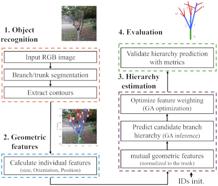
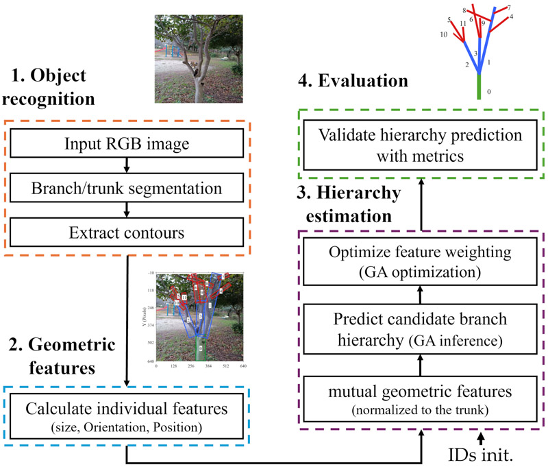
Fig. 1. Proposed pipeline for geometric and hierarchical modeling to support automated pruning; branch detection is visualized with bounding boxes for clarity.
The methodology of the proposed automated pruning decision system consists of four phases: object recognition, individual feature extraction, hierarchy estimation, and validation (Fig. 1). Initially, a single RGB image of a tree was analyzed using a custom YOLO model to segment the branches and trunk. Subsequently, the individual features of the branches and trunk were extracted by analyzing the segmented output using the PCA. These features included the length and width in pixels, angle in degrees, and coordinates of the start, center, and end points. These geometric descriptors capture the structural relationships of branches, providing information for subsequent pruning-related analyses. The pixel-based dimensions were normalized to trunk values, where a GA was employed to determine parent-child relationships by assessing geometric feature differences, which were represented as mutual features, and fine-tuning the prediction thresholds. The GA was initialized once using hierarchy-based branch identifiers as ground-truth references, while subsequent relationship inference relied primarily on geometric features due to their higher stability.
Finally, the validation phase evaluates the performance against the actual hierarchy by calculating various metrics and comparing them with non-optimized fixed-rule thresholding. This process enables the accurate modeling of tree structures and ensures biologically safe pruning decisions during scans, which supports long-term tree health and productivity.
The pruning decision process represents a crucial subsequent stage but is beyond the scope of the present framework; therefore, it is not illustrated in Fig. 1. However, it is briefly addressed in Section 4. The following sections provide detailed explanations of each stage of the study.
By integrating vision-based detection with the YOLOv8-seg model, PCA-driven geometric feature extraction, and GA-based hierarchical inference, this study establishes a unified pipeline that links advanced computer vision with horticultural principles. YOLOv8-seg provides robust segmentation of trunks and branches; PCA condenses contour data into key geometric descriptors; and the GA infers parent-child relationships to reconstruct biologically meaningful hierarchies. This design ensures that pruning decisions are guided by both geometric accuracy and botanical logic, offering a reliable and scalable foundation for robotic pruning systems capable of consistent and safe operation across various conditions.
It is important to note that the proposed approach is designed as a geometry- and hierarchy-driven perception module and does not rely on species-specific traits, training systems, or orchard-dependent assumptions. Instead, it infers parent–child relationships from generic structural cues, such as branch size, orientation, and attachment geometry, which are common across a wide range of tree types. In this study, urban trees, characterized by less controlled growth patterns and higher structural variability, are deliberately used as a challenging proxy, providing a conservative evaluation compared to orchard trees that are typically trained and pruned to maintain regular architectures. Accordingly, while the approach is motivated by orchard pruning applications, it is formulated as a foundational perception layer that can be integrated with task-specific pruning planners in future autonomous orchard deployments.
3.1. Object Recognition
Accurate segmentation of the branches and trunks is the basis for subsequent geometric feature extraction and hierarchical estimation. The YOLOv8-seg model was selected because of its high detection accuracy and suitability for real-time applications 23,24,25. This makes it ideal for automated pruning tasks, where occlusions, light variations, and complex backgrounds are prevalent. To enable trunk and branch segmentation using the YOLOv8 segmentation model (YOLOv8-seg), a dataset of approximately 2000 high-resolution images was collected and annotated. Owing to their accessibility, diverse branching patterns, and shared fundamental structural characteristics with orchard trees, images were captured in urban areas under varying conditions of obscuration, camera perspectives, distances, background complexity, and brightness. The diversity in brightness exposes the segmentation model to natural lighting variability commonly encountered in outdoor environments and enhances its robustness when analyzing orchard trees under different lighting conditions.
Fig. 2. Data annotation process for YOLOv8 segmentation.

Fig. 3. Schematic representation of the YOLOv8 segmentation model training process (adapted from 26).
Dataset preparation for YOLOv8-seg training involved a systematic annotation process. As illustrated in Fig. 2, the process consists of several steps: image acquisition, manual annotation of branch and trunk structures, resizing of annotated images to a standardized input size, and compilation of the processed images into the final training dataset. Annotation was performed using Roboflow, with polygons encircling the visible branches. The emphasis was on distinguishing the main branch from its offspring or any overlapping branches to investigate hierarchical structures. Fig. 3 shows the training process for the annotated dataset. It begins with a backbone network, a convolutional neural network responsible for extracting features from input images, such as visual patterns that distinguish branches from the background of an image. The neck layer, implemented as a feature pyramid network (FPN), refines these features across multiple scales to detect branches of different sizes.
The head layer uses the accumulated features to assign class labels and generate bounding boxes and mask contours for each detected branch. Ultimately, the predicted output was compared with the annotations in the training set to calculate the loss functions, which assisted the model in improving its segmentation and detection abilities 27,26.
As indicated in our previous study 28, branch recognition remained stable across varying environmental conditions, detecting nearly all branches with a correct detection rate of 0.99 at low confidence thresholds (0.05) and avoiding false detections until thresholds of (0.1–0.3).
These results indicate that the recognition stage remains resilient to illumination variations, providing stable branch detection and a reliable visual foundation for subsequent geometric and hierarchical analysis. The current model exhibited a similar behavior, maintaining consistent detection and ensuring that the recognition phase provided a reliable basis for the hierarchical analyses.
3.2. Geometric Feature Extraction
Analyzing branch geometry and hierarchical relationships requires dimensionality reduction to manage the contour data produced by YOLOv8-seg, which frequently incorporates redundancy and irregularities.
In this context, PCA was employed to identify the dominant features 29, which were then used in a GA-based approach to model parent-child relationships. The following section provides an overview of PCA and highlights its significance in the analysis of geometric structures.
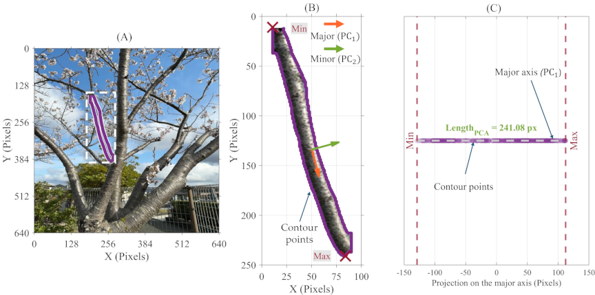
Fig. 4. PCA-based branch length estimation from an RGB image: (A) segmentation, (B) axis extraction, and (C) length projection.
3.2.1. Concept of PCA
Principal component analysis (PCA) is a statistical technique that reduces data complexity by transforming correlated variables into a smaller set of uncorrelated principal components.
In the case of 2D contour data, only two principal components are involved. These components represent the most significant variations in the original data, facilitating the analysis 30.
In geometric analysis, PCA offers a valuable method for representing the dominant features of each branch and trunk contour by analyzing their spatial distributions and directions. These aspects are crucial for guiding pruning decisions and understanding the hierarchical relationships in the subsequent sections. The application of PCA to branch and trunk contour data is based on standard mathematical definitions. For clarity and conciseness, the mathematical details are omitted, and the focus is placed on the geometric features extracted from PCA.
Although analyzing the spread along the principal axes provides a valuable perspective on branch geometry, it does not directly relate to geometric dimensions, such as length and width. To translate these findings into a quantitative metric, the following sections discuss how to estimate the values of the length, width, and other geometric properties using contour data and the PCA concept. Because contour data often contains irregularities caused by occlusion or segmentation noise, we compared the PCA-based method with conventional geometric approaches. This comparison confirmed that PCA yielded reliable estimates of branch length, width, and orientation, even from imperfect contours, offering a unified approach for tree geometry analysis.
3.2.2. Length Estimation with PCA
Branch length informs pruning decisions by reflecting branch size and the impact of cutting. In addition, this enables the distinction between primary and higher-order branches. Therefore, this knowledge contributes to hierarchy estimation.
In this study, all branch dimensions are reported in pixel units rather than physical dimensions, as our approach focuses on the relative relationships between branches.
According to the PCA principles, the first axis (major axis) represents the branch’s longitudinal extent, which forms the basis for the length estimation. In the following section, we assess the consistency of this length calculation by comparing it with a conventional geometric method that uses the Euclidean distance (ED method) between the two most distant points on the branch contour.
For the PCA-based approach, the branch length is estimated by calculating the range of projections along the major axis, by subtracting the minimum projected value from the maximum projected value, as shown in Eq. \(\eqref{eq:1}\):
Figure 4 illustrates the method to measure branch length using PCA. The branch contour was extracted from the original RGB image (Fig. 4(A)). Next, PCA identified the major and minor axes (Fig. 4(B)).The minimum and maximum projection points along the major axis were then computed to represent the estimated length. By plotting the projected contour points on the major axis (Fig. 4(C)), the endpoints indicate the branch length.
In the ED method, the distance between all pairs of contour points \([i,j]\), is calculated as Eq. \(\eqref{eq:2}\):
The comparison in Fig. 5 demonstrates how PCA-based length estimation was evaluated against the ED method. Preliminary analyses across representative branches showed strong agreement between the two approaches, indicating that branch length was captured consistently.
This step was included to validate the robustness of PCA as a unified basis for geometric extraction. A more extensive analysis of a larger set of branches is provided in Section 4.
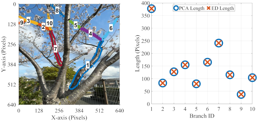
Fig. 5. Comparison of length estimation for PCA and ED methods.
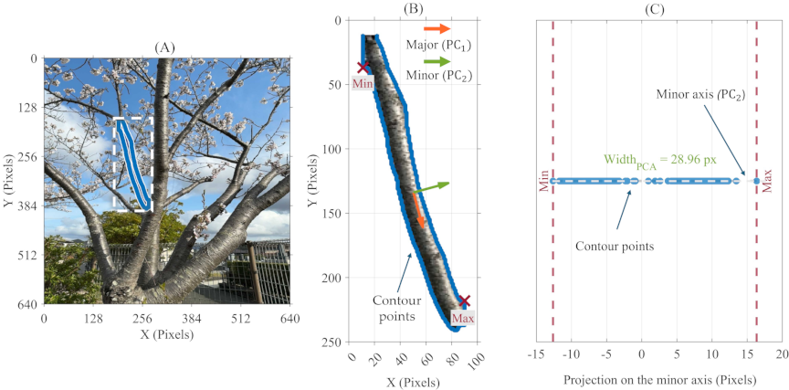
Fig. 6. PCA-based branch width estimation from an RGB image: (A) segmentation, (B) axis extraction, and (C) width projection.
3.2.3. Width Estimation with PCA
Width indicates mechanical strength, guiding pruning decisions and hierarchy, as parents are generally wider. The second axis of PCA indicates the lateral dimension of the branch, which is used to estimate the width.
In the following section, we compare the consistency of the PCA-based width estimation with that of a conventional geometric approach, where each branch is enclosed within the smallest possible rectangle (minimum area rectangle, MAR).
The minimum Euclidean distance was not used for width because it may measure adjacent points on the contour rather than opposite points, failing to represent the true branch thickness.
For the PCA-based method, branch width is obtained as the range of projections along the minor axis (\(\mathrm{PC}_{2}\)), as expressed in Eq. \(\eqref{eq:3}\):
Figure 6 illustrates the method used to measure branch width using PCA. Similar to the length calculation, width is obtained as the range of projections along the minor axis (\(\mathrm{PC}_{2}\)), with the endpoints of the projected contour points indicating the estimated width.
For the MAR method, a geometric method was used to estimate the branch width by fitting a minimum area rectangle around each contour.
This method involves finding the smallest rectangle that completely encloses a given perimeter. The lengths of the two perpendicular sides of this rectangle are calculated, and the width of the branch, in this case, is the measure of the shorter side. Fig. 7 illustrates the MAR process flowchart.

Fig. 7. Flow chart of the MAR method for estimating the branch width.
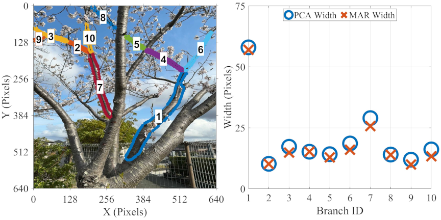
Fig. 8. Comparison of width estimation for PCA and MAR methods.
As shown in Fig. 7, the process begins with inserting the contour extracted from the YOLOv8-seg model. Then, the smallest rotated rectangle enclosing the contour is found by OpenCV’s cv2.minAreaRect(), which returns two perpendicular side dimensions. The shorter side is used for branch width estimation as Eq. \(\eqref{eq:4}\):
Figure 8 shows a comparative evaluation of branch width estimation using PCA-based and MAR-based methods across several illustrative branches.
This comparison demonstrates that PCA- and MAR-based methods capture the expected pattern of branch width, with parent branches being thicker than their child branches. Minor differences between the two methods are discussed in Section 4.
3.2.4. Position Estimation with PCA
Estimating branch position coordinates is necessary to capture their spatial relationships, which are later used for hierarchy, pruning decisions, and execution. PCA was applied to the contour points of the trunk and each branch. The two extreme projections along the major axis define the start point \(S\) and endpoint \(E\). The center point \(C\) is then defined as the geometric midpoint. The complete procedure is summarized in Algorithm 1.

This approach uses the trunk as a reference to resolve ambiguity between branch start and end points, consistent with the natural growth pattern in which branches originate near the trunk.
3.2.5. Orientation Estimation with PCA
Orientation describes how branches extend from the trunk and from one another, influencing accessibility and growth response, while also indicating parent–child relationships within the branching structure.
As discussed in Sections 3.2.2 and 3.2.3, PCA has demonstrated the capability to diagnose the spread direction, which in turn allows for the measurement of the branch’s elongation direction.
In the following section, we evaluate the consistency of the angle calculation based on PCA and compare it with a geometric method that uses the axis formed by the two farthest points of the contour data (FP method).
To ensure that both methods reflected biologically realistic growth patterns, we applied a half transformation that oriented the branch angles upward.
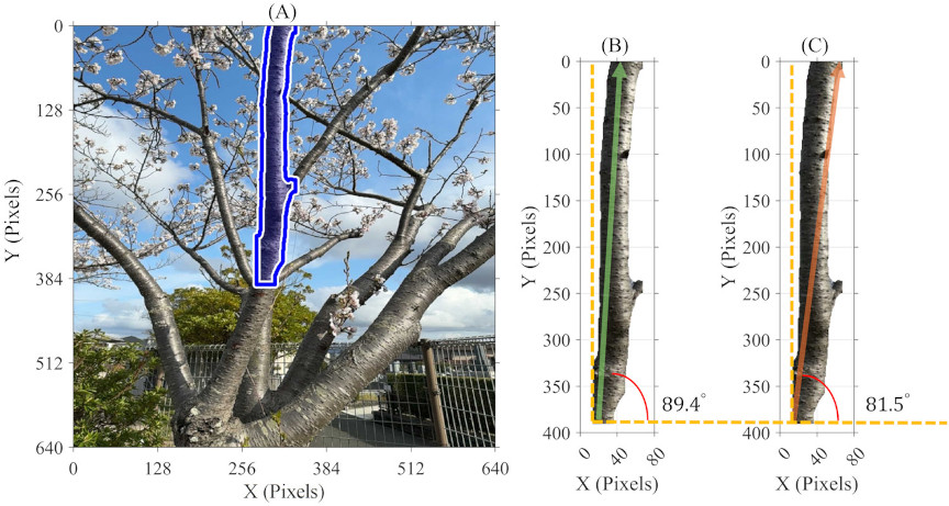
Fig. 9. (A) Tree with branch contour. (B) PCA axis (green), vertical reference (dashed orange), and angle (red arc). (C) Farthest-point axis with vertical reference and angle.
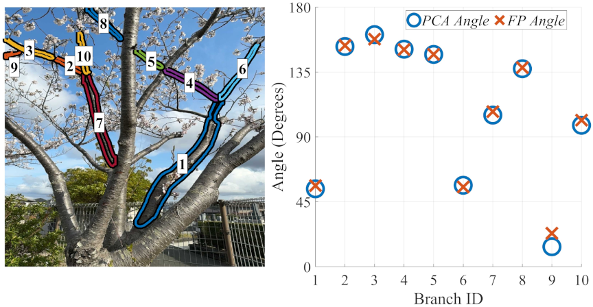
Fig. 10. Comparison of angle estimation for PCA and FP methods.
For the PCA-based approach, the branch angle is estimated by calculating the angle of the major axis (\(\mathrm{PC}_{1}\)), according to Eq. \(\eqref{eq:5}\):
For the farthest point (FP) method, the Euclidean distance is computed for all pairs in the contour data, and then the pair \((p_2,p_1)\) is found by Eq. \(\eqref{eq:6}\):
Figure 9 provides a visual overview of the workflow used to extract the branch orientation using the PCA-based and FP-based methods. After extracting the branch contour from the RGB image, each method determines an axis: PCA finds the direction of the maximum variance, whereas FP connects the two most distant points along the contour.
Figure 10 illustrates the preliminary comparison between the PCA and FP methods used to estimate branch orientation. For straight branches, both methods yielded identical values, whereas slight deviations were observed for curved branches. A more extensive analysis of a larger set of branches is presented in Section 4.
After extracting the branch characteristics using PCA, the length, width, and orientation were consistently derived from the branch contours. In addition, the positional coordinates, namely the start point, center point, and endpoint of each branch, were estimated from projections onto the principal axes.
Together, these geometric and positional descriptors provide mutually comparable features that enable the quantitative assessment of potential parent–child relationships among branches. Although the preliminary results did not differ substantially from conventional geometric methods, PCA was adopted as a unified pipeline for geometric parameter extraction, which subsequently served as the basis for hierarchical prediction.
3.2.6. Mutual Features Extraction
Once the geometric features are extracted, they are quantitatively compared through mutual feature analysis to evaluate their suitability as inputs for algorithms that identify parent–child branch relationships using thresholds optimized from geometric characteristics.
The mutual features include morphological features, including the width difference (\(\Delta W\)), length difference (\(\Delta L\)), and angle difference (\(\Delta \theta\)), while the attachment features include distance from the end of a branch/trunk to the start of another branch (\(d_{\mathit{ES}}\)), distance from the center to the center (\(d_C\)), and two directional attachment offsets; the parallel offset (\(d_{\parallel}\)) and the perpendicular offset (\(d_{\bot}\)). Algorithm 2 provides a complete procedure for the extraction of the mutual features. As defined in Algorithm 2, trunk normalization was applied to ensure scale-invariant cues by expressing widths, lengths, and spatial offsets relative to the trunk.

Morphological features capture distinctions in both size and orientation. \(\Delta W\) reflects thickness variation, where significant deviations may indicate a structural disconnection. \(\Delta L\) emphasizes morphological accuracy, with upper-level branches usually being shorter. \(\Delta \theta\) reflects the extent to which the direction of a child branch deviates from its parent. Together, these features form common structural descriptors used in tree modeling 31 and are used as input to characterize hierarchical connectivity.
The pair (\(d_{\parallel}\), \(d_{\bot}\)) disambiguates axial versus lateral relationships: in the case of \(d_{\parallel} \gg d_{\bot}\), This suggests that the candidate segment is likely a direct or higher-order child of this parent branch, whereas \(d_{\parallel} \ll d_{\bot}\) may indicate a lateral neighbor rather than a child.
In practice, to further ensure uniqueness, we prioritize the candidate with the smallest distance within a reasonable axial window, thereby minimizing false links to nearby side branches. Due to potentially noisy or overlapping endpoints, we also incorporate the center-to-center distance \(d_{C}\) as a global validation criterion.
Figure 11 illustrates the concept of parallel-perpendicular decomposition for branch attachment. Depending on branch geometry, some features provide stronger cues than others, and their importance is optimized in the hierarchy estimation.
Following mutual feature extraction (Algorithm 2), a GA was used to learn decision thresholds that improve parent–child prediction accuracy and hierarchical inference.
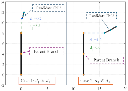
Fig. 11. Parallel–perpendicular decomposition for branch attachment.
3.2.7. GA
GA is optimization technique inspired by the principles of natural selection. GA searches for a population of candidate solutions through processes such as selection, crossover, and mutation to maximize or minimize an objective function 32. Because GA does not require gradient information and can handle non-differentiable objectives and bounded parameters, it is well-suited for threshold optimization problems. GA has been used to solve several optimization problems 33,34.
Our approach is based on defining thresholds for each mutual feature and then treating these thresholds as variables that must be optimized to maximize the accuracy of predicting the true parent-child links. The set of thresholds was defined by Eq. \(\eqref{eq:9}\):
The optimization problem in Eq. \(\eqref{eq:11}\) is solved using GA, which is applied independently across multiple hierarchical levels, for instance, the hierarchical level that describes the relationship between the trunk and the branches that connect directly to it (trunk \(\to\) primary branches). For each threshold of the \(T\) set, the search space is bounded by the minimum and maximum mutual features to ensure acceptable output values.
To increase robustness against noisy or missing features, a minimum agreement (MinAgree) rule was applied, whereby a parent-child pair \((i,j)\) is predicted as a link if at least \(m\) of the mutual features satisfy their required thresholds. According to Eq. \(\eqref{eq:12}\):
For each candidate threshold set, the MinAgree value is applied to predict parent–child relationships, and the Jaccard index is computed by comparing the predicted links with the ground truth, serving as the fitness measure. Threshold sets with higher Jaccard scores are selected for further refinement.
In the GA configuration, each chromosome encodes a vector of feature thresholds together with the MinAgree parameter. An initial population of random chromosomes is generated within the defined bounds.
Crossover is performed using an intermediate crossover operator, producing offspring located between parent chromosomes, expressed as Eq. \(\eqref{eq:13}\).
While feasible adaptive mutation introduces small random perturbations to maintain diversity. An appropriate population size ensures both exploration and convergence. During optimization, the GA evaluates MinAgree values in the range of 1–7 and selects the value that maximizes the Jaccard index. This evolutionary cycle continues until the convergence criteria are met. The overall process is illustrated in Fig. 12.

Fig. 12. Flowchart of the GA for optimal threshold selection and parent-child relationship prediction (adapted from 32).
3.3. Experimental Setup
3.3.1. Geometric Estimation Experiment
The geometric performance of the proposed algorithm was evaluated across approximately 200 branches from 10 different trees in urban areas in Fukuoka, Japan. Although the trees were not part of a managed orchard, they were selected because the study focused on geometric properties common to all tree types, such as branch length, width, and orientation; therefore, the employed data were sufficient and appropriate for evaluating geometric feature extraction.
Branch contours were extracted using the custom YOLO model, and geometric features, including the length, width, and angle, were estimated. The primary objective of this evaluation was to demonstrate the ability of PCA-based approach to consistently capture branch size and orientation. PCA-based estimates were compared with the described methods using the standard deviation \(\sigma\) and correlation coefficient \(r\).
3.3.2. Hierarchy Estimation Experiment
Our methodology focuses on the tree hierarchy across two depth levels using a GA optimized by the Jaccard index. The first level addresses the separation between the trunk and primary branches, which is critical for identifying the main structure of the tree. The second depth level extends this separation to distinguish secondary branches from their corresponding primary branches, enabling a finer hierarchical resolution that supports selective pruning and operation sequencing.
The proposed algorithm was evaluated on five trees exhibiting varied branching structures. The evaluation was designed as a proof-of-concept study, focusing on hierarchical inference from geometric properties common across tree types, including relative length, width, orientation, and spatial attachment. Accordingly, the selected data provides an adequate and representative basis for validating the proposed hierarchical reasoning approach.
To enhance clarity, the hierarchical structure of the first tree is described in detail and used as a representative example for explaining methodology. The performance of the proposed GA-based thresholding approach is then evaluated across all five trees and compared against a fixed-threshold baseline, highlighting the limitations of fixed rules and demonstrating the advantage of learned thresholds for robust hierarchy estimation.
As illustrated in Fig. 13, the trunk was identified as zero, which is highlighted in green; primary branches (identifiers 1–3) are highlighted in blue, and secondary ones (identifiers 4–11) are highlighted in red. These data collectively serve as the ground truth for evaluating the proposed hierarchical estimation method in the following sections.
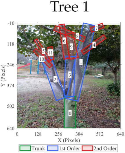
Fig. 13. Hierarchical annotation of Tree 1 using bounding boxes to visually emphasize branch levels.
The GA was applied to two separate sets of nodes: first level of hierarchy (Level 1 links), from the trunk to the primary branches; and (Level 2 links), from the primary to the secondary branches.
This separation aims to detect differences between the two levels during the optimal threshold learning process while preserving their distinct structural properties. As mentioned, the objective was to optimize the Jaccard index between the predicted and actual parent-child relationships. The learned thresholds were subsequently used to reconstruct the tree structure.
For both levels, mutual features, such as \(\Delta W_{ij}\), \(\Delta L_{ij}\), \(\Delta\theta_{ij}\), \(d_{\mathit{ES},ij}\), \(d_{C,ij}\), \(d_{\parallel,ij}\), and \(d_{\bot,ij}\) for every candidate pair \((i\to j)\), were extracted using the contours of objects (branches and trunk). The parent–child relationships were then manually assigned. A population size of 500 over 1,000 generations, with fault tolerance of \(10^{-5}\), was applied.
Because GA is stochastic (random initial population, selection, crossover, and mutation), a single run can reach a different local optimal value depending on the random seed. To make the solution robust and reproducible, we repeated the training using 0–200 independent seed points. This multi-seed sweep reduces the initialization sensitivity, producing thresholds that generalize more effectively. Table 1 summarizes the GA training setup used in this study.
Figure 14 shows the remaining four experimental trees using segmentation-based visualization. Together with Tree 1, these trees were used to demonstrate the effectiveness of the proposed method in comparison with a fixed-rule threshold approach. Here, a fixed-rule threshold refers to using a single geometric cue, such as distance or angle, with a constant threshold to infer branch relationships, where the threshold value is selected empirically and applied uniformly across all trees.
Table 1. GA configuration for maximizing Jaccard similarity of branch links.

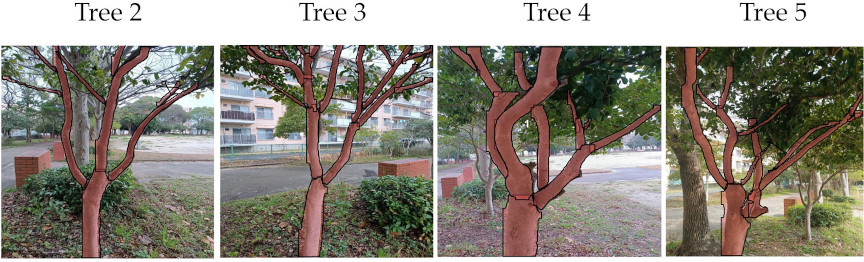
Fig. 14. Visualization of the four additional trees for comparison with fixed-rule thresholding.
4. Results and Discussion
After describing the experimental data used in geometric and hierarchical estimation, the following section presents the results.
4.1. Geometric Estimation
Table 2 summarizes the findings of comparison metrics, including the correlation \(r\) and standard deviation \(\sigma\). Correlation captures the consistency of trends across the methods, ensuring that PCA follows the same structural patterns as the geometric methods. Simultaneously, \(\sigma\) highlights the stability of the differences.
The PCA-based width estimation method correlated closely with the MAR method (\(r=99.6\)), resulting in a low variance (\(\sigma=1.42\) px), this difference can refer to the curved or irregular shape of some branches. The PCA-based branch length estimation method was nearly identical to the ED method, with a near-perfect correlation (\(r=99.9\)) and negligible deviation (\(\sigma=0.49\) px). Similarly, the PCA-based angle estimation method closely matched the FP method (i.e., \(r=99,7\), \(\sigma=4.11°\)).
Based on the overall comparison, the small differences indicate that PCA-based methods are sufficiently robust as a unified approach for capturing branch shape and orientation required for hierarchical estimation, providing a reliable basis for subsequent pruning decisions.
4.2. Tree Level Separation
As mentioned earlier, this experiment aims to demonstrate the ability to separate the hierarchical levels of the defined Tree 1 based on the estimated mutual features. Fig. 15 shows the average of the optimized thresholds \(T^{\ast}\) using seeds from 0 to 200 for seven signals, including \(\Delta W\), \(\Delta L\), \(\Delta\theta\), \(d_{\mathit{ES}}\), \(d_C\), \(d_{\parallel}\), and \(d_{\bot}\). The value of MinAgree increased from 1 to 7. As a function of the MinAgree index, the results revealed distinct patterns that distinguished Level 1 and Level 2 links.
For Level 1, the thresholds remained consistently compressed across all attributes, with \(\Delta\theta \le 15°\), \(\Delta W\le 0.2\), and \(\Delta L\le 1\). This confirmed the geometric stability and regularity of the trunk attachments. Meanwhile, the Level 2 thresholds expanded significantly, reflecting the irregularity of secondary growth, approximately \({20°} \le \Delta\theta \le {70°}\), \(0.4\le \Delta W\le 0.65\), and \(0.6\le\Delta L\le 1.8\).
Although the distance features were more stable than the geometric signals, they also demonstrated a clear upward shift at Level 2. The findings in Fig. 15 confirmed the robustness of the proposed approach in enforcing Level 1 similarity and accommodating broader Level 2 variability.
Although some thresholds were close to each other for specific features and values, this closeness is likely to play a significant role in separating false links, which are analyzed in the following sections.
Table 2. Consistency between PCA-based and geometric feature extraction methods.

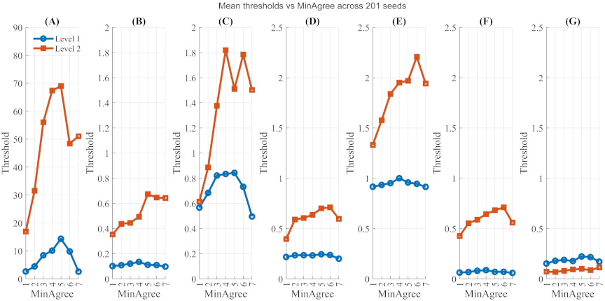
Fig. 15. Mean threshold variation with MinAgree across various seeds for Level 1 and Level 2 links. (A) \(\Delta \theta\), (B) \(\Delta W\), (C) \(\Delta L\), (D) \(d_{\mathit{ES}}\), (E) \(d_C\), (F) \(d_{\parallel}\), and (G) \(d_{\bot}\) for defined Tree 1.
4.3. Hierarchical Estimation
While Fig. 15 demonstrates the algorithm’s ability to find thresholds to maximize the Jaccard index for different values at Levels 1 and 2, this value reflects only the isolated learning threshold. To fully assess the robustness of the proposed approach, hierarchical validation must consider both levels together, starting from the trunk (\(\textrm{ID} = 0\)), which was treated as the reference parent. The thresholds set \(T_{L1}^{\ast}\) learned during training on Level 1 were applied to all candidate child branches (\(\textrm{ID} = 1\) to 11). A parent-child relationship was accepted if at least MinAgree of the seven mutual features are within their learned bounds. The predicted Level 1 children were then treated as parents in the second stage of validation, where the threshold set \(T_{L2}^{\ast}\) was applied to their outgoing links. Thereafter, ground truth was utilized to compute precision, recall, F1 score, and Jaccard index. Precision measures the proportion of correctly predicted links among all predicted links, recall measures the proportion of true links that were correctly identified, and F1-score combines both into a single balanced indicator 36. The procedure for the validation algorithm is shown in Algorithm 3.
Figure 16 illustrates the effect of the MinAgree threshold on the overall performance of hierarchical validation, evaluated by combining Levels 1 and 2 while gradually increasing the MinAgree threshold from 1 to 7. As illustrated, increasing MinAgree leads to a steady enhancement in precision, which peaks at \(\textrm{MinAgree} = 6\), indicating a reduction in false detections under stricter agreement criteria.
However, recall exhibits an early peak around \(\textrm{MinAgree} = 2\)–3 before gradually declining, suggesting that overly strict thresholds may lead to missed true links. Both the F1 score and the Jaccard index follow a balanced trend, improving consistently up to MinAgree at 5–6, where they achieve their highest values before dropping sharply at \(\textrm{MinAgree} = 7\). These results suggest that moderate MinAgree values 4–6 provide the best trade-off between precision and recall, supporting robust hierarchical validation.
The next section delves into an ablation analysis of the model to assess the contribution of mutual features.
4.4. Feature Importance via Ablation
This analysis underscores the relative significance of geometric and distance-based cues to the overall hierarchical estimation. The predictive significance of each mutual feature was quantified by the average reduction in the Jaccard index when that feature was removed.
As shown in Fig. 17, \(d_{\parallel}\) produced the largest drop in performance, confirming that parallel distance is the most critical factor in establishing reliable parent–child branch relationships for this tree. Length \(\Delta L\) and endpoint separation \(d_{\mathit{ES}}\) followed closely, indicating that elongation and convergence relationships also play an important role in maintaining structural consistency.
In contrast, \(d_C\), \(d_{\bot}\), and \(\Delta W\) exhibited moderate contributions, suggesting that these cues help refine the hierarchy but are not dominant on their own. The angle difference \(\Delta\theta\) was the least influential overall, though its contribution became more relevant when combined with other geometric features.
Taken together, these findings show that while the framework integrates a mixture of geometric and distance-based signals, axial alignment and spatial positioning cues remain the most reliable indicators for reconstructing the tree hierarchy. This balance of features provides robustness against structural irregularities and ensures representation of branching patterns, which is essential for enabling safe pruning.
It is important to note that the effectiveness of this validation may differ depending on species growth patterns and seasonal variations, since they exhibit diverse branching behaviors influenced by age, environment, and horticultural practices. These variations highlight the need for adaptive robotic systems that update their models to stay reliable under real orchard conditions.

4.5. Pruning Suggestions from Geo-Hierarchical Visualization
This section displays predictions in terms of false positives (FP), which indicate incorrect links; false negatives (FN), which indicate missing links; and true positives (TP), which indicate correct links. Together, these metrics provide an intuitive view of how the tree hierarchy is constructed, while simultaneously revealing the contribution of geometric cues such as branch angle, length, and width related to pruning decisions.
Figure 18 shows the representation of the hierarchy and estimation under different thresholds. The top row shows the original tree and its annotated hierarchy, whereas the bottom panels show the reconstructed structures, along with the corresponding evaluation metrics.
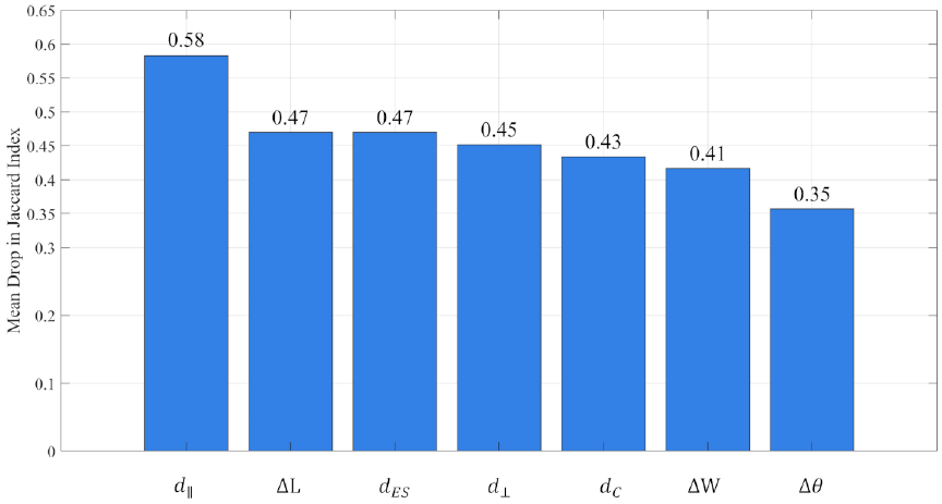
Fig. 16. Effect of MinAgree threshold on overall hierarchical validation accuracy for the defined Tree 1.
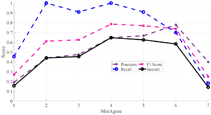
Fig. 17. Mean drop in Jaccard index for MinAgree thresholds ranging from 1 to 7 for the defined Tree 1.
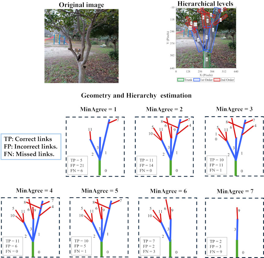
Fig. 18. Hierarchy representation. Only the correctly predicted links TP are plotted, while FP and FN are reported in the text boxes.
The results are discussed from several perspectives. First, considering the effect of MinAgree, for \(\textrm{MinAgree} = 1\), the number of TP was relatively low with higher FP and FN. This reflects the difficulty in discerning the hierarchical structure when the number of constraints is low, leading to a poor appreciation of the tree topology. For moderate values (\(2 \le \textrm{MinAgree} < 4\)), the number of TP increased, whereas the FP decreased. The best performance was observed at \(\textrm{MinAgree} = 4\), where the reconstructed hierarchy was closest to the ground truth with minimal errors. Higher values (\(5 \le \textrm{MinAgree} < 7\)) further reduced false positives, but at the cost of missing true links. \(\textrm{MinAgree} = 7\) eliminated most of the links. These findings highlight the necessity of integrating multiple learned geometric thresholds rather than fixed, non-optimized single thresholds to achieve a robust visualization of the tree structure.
From the perspective of a pruning robot, accurately reconstructing the branch hierarchy is essential for making safe and effective decisions. Identifying branches 1, 2, and 3 as Level 1 branches with respect to the trunk indicates that these form the primary scaffold of the tree; therefore, pruning these branches is performed more cautiously and strategically than pruning higher-order branches.
Furthermore, hierarchical information can support the planning and execution of pruning actions. From an operational perspective, recognizing that a branch is structurally connected to subordinate branches enables coordinated cutting strategies, which may reduce redundant cutting motions and help minimize mechanical stress at the branch junctions during execution.
Geometric reasoning plays a complementary role in reinforcing pruning decisions, as vertical branches may indicate potential co-dominance with the trunk, whereas long and slender branches may serve as indicators of increased susceptibility to failure.
Table 3. Comparison of hierarchy estimation performance across the five defined trees. J refers to the Jaccard index.

4.6. Hierarchical Depth and Fixed-Rule Thresholding
This section discusses the hierarchical depth selection and fixed-rule thresholding for structural inference across the five evaluated trees. Two hierarchical depth configurations were considered in this study. Level 1 is related to trunk-primary branch relationships, while Level 2 considers both trunk-primary and primary-secondary branch relationships. These two levels correspond to the most critical stages for pruning-oriented perception, as they are directly related to identifying scaffold branches and their immediate descendants, which form the structural backbone of the tree.
At the first hierarchical depth, the trunk must be separated from the primary branches, which typically exhibit strong geometric contrasts in terms of length, width, and attachment position. As shown in Table 3, the fixed-rule approach achieved a mean F1 score of 0.54 and a Jaccard index of 0.39, indicating moderate performance when the geometric separation was pronounced. In contrast, the proposed adaptive method achieved near-perfect performance at this level, with a mean F1 score of 0.99 and a Jaccard index of 0.97, consistently, across all five trees. This result highlights the importance of reliably identifying scaffold branches, as errors at this level would propagate to deeper hierarchy inference and compromise subsequent pruning-related reasoning.
At the second hierarchical depth, the challenge increases substantially because the geometric differences between the primary and secondary branches are more subtle and less consistent across trees. This effect is clearly reflected in the performance of the fixed-rule baseline, which shows a sharp drop to a mean F1 score of 0.28 and a Jaccard index of 0.16. The large variability observed across trees at this depth indicates that a single fixed threshold is insufficient to capture the diverse geometric configurations present in the different tree structures. In contrast, the proposed GA-based approach maintained a strong performance at the second depth, achieving a mean F1 score of 0.83 and a Jaccard index of 0.71, demonstrating its ability and highlighting the importance of adapting thresholds to tree-specific geometries.
Overall, the results in Table 3 demonstrate that adaptive, multi-threshold learning is essential for stable hierarchy estimation across multiple trees and depth levels, whereas fixed rule exhibits limited robustness.
5. Conclusion
This study presents a geometry- and hierarchy-driven inference framework for reconstructing tree structures using multiple geometric and distance-based cues extracted by principal component analysis (PCA). PCA effectively detected structural differences in branch length, width, and orientation, whereas GA-based estimation achieved reliable branch separation by adaptively combining multiple thresholds, maintaining a balance between precision and recall. Although the current implementation is limited to estimating the hierarchy from a single image, which can fail for complex or irregular growth tree structures, it provides a computationally efficient and easy-to-use perception layer suitable for orchard trees, where growth is relatively controlled. In contrast, 3D methods, such as LiDAR or depth sensing, provide richer structural details but often require larger scans, additional sensors, and more complex computations.
Future work will extend the proposed approach to a wider range of tree structures. While structural pruning is commonly recommended when the tree architecture is clearly visible 12, this system will be further developed to improve robustness under dense foliage and varying illumination. This includes incorporating additional cues, such as depth and curvature; studying adaptive threshold learning at the level of tree groups or orchard blocks to reduce per-tree optimization; exploring alternative optimization strategies, such as simulated annealing or particle swarm optimization; and integrating the proposed perception system with robotic platforms, where geo-hierarchical inference can support safe and efficient pruning decisions.
Author Contribution M. A. led the conceptualization, methodology, formal analysis, software implementation, and drafting of the manuscript. R. A. contributed to the discussion and refinement of the methodology. I. I. provided key input on the methodological use of PCA. S. P. contributed to the debate, improved visualization, and provided support in experiments. A. A. supported the literature review and discussion. H. A. assisted with data analysis and manuscript structure. K. I. supervised the research and provided critical feedback.
Data Availability Statement Data is available from the corresponding author upon reasonable request.
Funding This research received no external funding.
Ethics Statement This study used tree images collected outdoors and did not require ethical approval.
Conflict of Interest The authors declare that they have no conflict of interest.
Acknowledgments
The authors sincerely thank the reviewers for their valuable comments and constructive feedback, which helped improve this manuscript.
- [1] D. Mason-D’Croz et al., “Gaps between fruit and vegetable production, demand, and recommended consumption at global and national levels: An integrated modelling study,” The Lancet Planetary Health, Vol.3, No.7, pp. E318-E329, 2019. https://doi.org/10.1016/S2542-5196(19)30095-6
- [2] K. Pawlak and M. Kołodziejczak, “The role of agriculture in ensuring food security in developing countries: Considerations in the context of the problem of sustainable food production,” Sustainability, Vol.12, No.13, Article No.5488, 2020. https://doi.org/10.3390/su12135488
- [3] G. Montanaro, C. Xiloyannis, V. Nuzzo, and B. Dichio, “Orchard management, soil organic carbon and ecosystem services in Mediterranean fruit tree crops,” Scientia Horticulturae, Vol.217, pp. 92-101, 2017. https://doi.org/10.1016/j.scienta.2017.01.012
- [4] M. Rodríguez-Entrena, J. Barreiro-Hurlé, J. A. Gómez-Limón, M. Espinosa-Goded, and J. Castro-Rodríguez, “Evaluating the demand for carbon sequestration in olive grove soils as a strategy toward mitigating climate change,” J. of Environmental Management, Vol.112, pp. 368-376, 2012. https://doi.org/10.1016/j.jenvman.2012.08.004
- [5] Ş. Alp and B. Mutlu, “Aesthetic and ecological characteristics of Prunus Taxa in landscape design: A Study in eastern and southeastern provinces of Türkiye,” Eurasian J. of Forest Science, Vol.11, No.3, pp. 116-136, 2023. https://doi.org/10.31195/ejejfs.1275740
- [6] T. L. Davenport, “Pruning strategies to maximize tropical mango production from the time of planting to restoration of old orchards,” HortScience, Vol.41, No.3, pp. 544-548, 2006. https://doi.org/10.21273/HORTSCI.41.3.544
- [7] L. Esche, M. Schneider, J. Milz, and L. Armengot, “The role of shade tree pruning in cocoa agroforestry systems: Agronomic and economic benefits,” Agroforestry Systems, Vol.97, No.2, pp. 175-185, 2023. https://doi.org/10.1007/s10457-022-00796-x
- [8] A. M. Dilla, P. J. Smethurst, N. I. Huth, and K. M. Barry, “Plot-scale agroforestry modeling explores tree pruning and fertilizer interactions for maize production in a Faidherbia parkland,” Forests, Vol.11, No.11, Article No.1175, 2020. https://doi.org/10.3390/f11111175
- [9] L. He and J. Schupp, “Sensing and automation in pruning of apple trees: A review,” Agronomy, Vol.8, No.10, Article No.211, 2018. https://doi.org/10.3390/agronomy8100211
- [10] S. Mei et al., “Current status of orchard mechanization technologies and key development priorities in the 15th Five-Year Plan period,” Int. J. of Agricultural and Biological Engineering, Vol.18, No.6, pp. 12-23, 2025. https://doi.org/10.25165/j.ijabe.20251806.9314
- [11] W. Liu, G. Kantor, F. De la Torre, and N. Zheng, “Image-based tree pruning,” 2012 IEEE Int. Conf. on Robotics and Biomimetics, pp. 2072-2077, 2012. https://doi.org/10.1109/ROBIO.2012.6491274
- [12] P. J. Bedker, J. G. O’Brien, and M. E. Mielke, “How to prune trees,” United States Department of Agriculture, 1995. https://doi.org/10.5962/bhl.title.98699
- [13] Aneja N. M. et al., “Pruning in horticulture: A blend of art and science,” J. of Scientific Research and Reports, Vol.30, No.10, pp. 313-329, 2024. https://doi.org/10.9734/jsrr/2024/v30i102458
- [14] L. Purcell, “Tree pruning essentials,” Purdue Extension, FNR-506-W, Purdue University, 2015.
- [15] A. Zahid et al., “Development of a robotic end-effector for apple tree pruning,” Trans. of the ASABE, Vol.63, No.4, pp. 847-856, 2020. https://doi.org/10.13031/trans.13729
- [16] M. Fernandes et al., “Grapevine winter pruning automation: On potential pruning points detection through 2D plant modeling using grapevine segmentation,” 2021 IEEE 11th Annual Int. Conf. on CYBER Technology in Automation, Control, and Intelligent Systems, pp. 13-18, 2021. https://doi.org/10.1109/CYBER53097.2021.9588303
- [17] Y. Yang et al., “Automatic method for extracting tree branching structures from a single RGB image,” Forests, Vol.15, No.9, Article No.1659, 2024. https://doi.org/10.3390/f15091659
- [18] S. Tong, J. Zhang, W. Li, Y. Wang, and F. Kang, “An image-based system for locating pruning points in apple trees using instance segmentation and RGB-D images,” Biosystems Engineering, Vol.236, pp. 277-286, 2023. https://doi.org/10.1016/j.biosystemseng.2023.11.006
- [19] A. You et al., “An autonomous robot for pruning modern, planar fruit trees,” arXiv:2206.07201, 2022. https://doi.org/10.48550/arXiv.2206.07201
- [20] F. Westling, J. Underwood, and M. Bryson, “A procedure for automated tree pruning suggestion using LiDAR scans of fruit trees,” Computers and Electronics in Agriculture, Vol.187, Article No.106274, 2021. https://doi.org/10.1016/j.compag.2021.106274
- [21] Y. Ban et al., “Monkeybot: A climbing and pruning robot for standing trees in fast-growing forests,” Actuators, Vol.11, No.10, Article No.287, 2022. https://doi.org/10.3390/act11100287
- [22] Y. Li and S. Ma, “Navigation of apple tree pruning robot based on improved RRT-Connect algorithm,” Agriculture, Vol.13, No.8, Article No.1495, 2023. https://doi.org/10.3390/agriculture13081495
- [23] A. Alraee, H. Alraie, M. Albaroudi, R. Alahmad, and K. Ishii, “Efficient ball position estimation for tennis court robot assistants using a dual-camera system,” Proc. of the 2025 Int. Conf. on Artificial Life and Robotics, pp. 378-381, 2025. https://doi.org/10.5954/ICAROB.2025.OS12-9
- [24] R. Alahmad et al., “Visual-based system for fish detection and velocity estimation in marine aquaculture,” Proc. of the 2025 Int. Conf. on Artificial Life and Robotics, pp. 351-355, 2025. https://doi.org/10.5954/ICAROB.2025.OS12-3
- [25] J. Lee and K.-I. Hwang, “YOLO with adaptive frame control for real-time object detection applications,” Multimedia Tools and Applications, Vol.81, No.25, pp. 36375-36396, 2022. https://doi.org/10.1007/s11042-021-11480-0
- [26] M. Hussain, “YOLOv5, YOLOv8 and YOLOv10: The go-to detectors for real-time vision,” arXiv:2407.02988, 2024. https://doi.org/10.48550/arXiv.2407.02988
- [27] P. Hidayatullah et al., “YOLOv8 to YOLO11: A comprehensive architecture in-depth comparative review,” arXiv:2501.13400, 2025. https://doi.org/10.48550/arXiv.2501.13400
- [28] M. Albaroudi, R. Alahmad, A. Alraee, and K. Ishii, “Evaluation of tree branch recognition algorithm in pruning robots under augmented environmental conditions,” Proc. of the 2025 Int. Conf. on Artificial Life and Robotics, pp. 356-360, 2025. https://doi.org/10.5954/ICAROB.2025.OS12-4
- [29] E. O. Omuya, G. O. Okeyo, and M. W. Kimwele, “Feature selection for classification using principal component analysis and information gain,” Expert Systems with Applications, Vol.174, Article No.114765, 2021. https://doi.org/10.1016/j.eswa.2021.114765
- [30] M. Greenacre et al., “Principal component analysis,” Nature Reviews Methods Primers, Vol.2, Article No.100, 2022. https://doi.org/10.1038/s43586-022-00184-w
- [31] W. Palubicki et al., “Self-organizing tree models for image synthesis,” ACM Trans. on Graphics, Vol.28, No.3, Article No.58, 2009. https://doi.org/10.1145/1531326.1531364
- [32] D. Waysi, B. T. Ahmed, and I. M. Ibrahim, “Optimization by nature: A review of genetic algorithm techniques,” The Indonesian J. of Computer Science, Vol.14, No.1, 2025. https://doi.org/10.33022/ijcs.v14i1.4596
- [33] C. Cavallaro, V. Cutello, M. Pavone, and F. Zito, “Machine learning and genetic algorithms: A case study on image reconstruction,” Knowledge-Based Systems, Vol.284, Article No.111194, 2024. https://doi.org/10.1016/j.knosys.2023.111194
- [34] S. Cateni, V. Colla, and M. Vannucci, “A genetic algorithms-based approach for selecting the most relevant input variables in classification tasks,” 4th UKSim European Symp. on Computer Modeling and Simulation, pp. 63-67, 2010. https://doi.org/10.1109/EMS.2010.23
- [35] L. D. F. Costa, “Further generalizations of the Jaccard index,” arXiv:2110.09619, 2021. https://doi.org/10.48550/arXiv.2110.09619
- [36] N. Aishwarya, K. M. Prabhakaran, F. T. Debebe, M. S. S. A. Reddy, and P. Pranavee, “Skin cancer diagnosis with Yolo deep neural network,” Procedia Computer Science, Vol.220, pp. 651-658, 2023. https://doi.org/10.1016/j.procs.2023.03.083
This article is published under a Creative Commons Attribution-NoDerivatives 4.0 Internationa License.