Paper:
Predictive Modeling of Crop Growth Using a Smart Agriculture Measurement Module Composed of Multipoint Soil Moisture Sensor and Environmental Sensors
Katsushi Ogawa
 , Wakana Ono, and Seonghee Jeong
Osaka Electro-Communication University
18-8 Hatsucho, Neyagawa-shi, Osaka 572-8530, Japan

In this study, we addressed agricultural labor shortages by developing a smart farming sensor module that integrated low-cost environmental sensors with a multipoint soil moisture sensor to predict broccoli growth, plant height (PH), and leaf count (Ln). Multivariable regression confirmed that integrated solar radiation (S) was the most dominant factor, although broccoli growth involved a complex interplay of solar radiation, optimal temperature, humidity, and soil moisture. More importantly, the analysis revealed that the middle layer soil moisture (um) exhibited the strongest positive contribution to PH. This finding indicated that water availability in the main root zone was essential for vertical growth and highlighted the indispensability of multipoint sensing over conventional single-depth measurements to accurately model the intricate relationship between soil moisture and crop development. Moving forward, we aim to leverage the superiority of multipoint data to construct a sophisticated growth prediction model, thereby contributing to the optimization of irrigation and temperature management in smart farming systems.
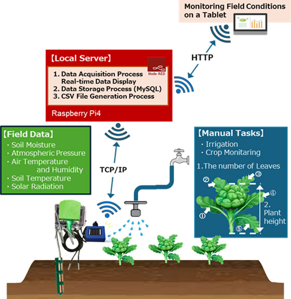
Conceptual diagram of the environmental monitoring system for broccoli growth in the field
1. Introduction
The global population is projected to reach 9.7 billion by 2050, raising concerns about the significant increase in food production 1. Consequently, irrigation is expected to remain a critical long-term challenge to meet the increasing global food demand, particularly in water-scarce regions. Irrigation plays a pivotal role in boosting crop yields and agricultural productivity, which are crucial for addressing this demand. Studies have reported that irrigation substantially improves crop water productivity and significantly contributes to increased food production 2,3. Therefore, irrigation is an indispensable component of agriculture, especially in arid and semi-arid regions with limited rainfall. Irrigation becomes essential during dry seasons with limited rainfall, even in humid or subhumid regions, to ensure an adequate water supply for crop growth 4. Water scarcity is a severe and prevalent issue in many regions. Conventional irrigation scheduling methods, which rely on manual scheduling based on crop observation, soil feel, and intuition, or using a timer control at predetermined intervals regardless of actual crop needs, often lead to high operational costs and inefficient water usage 5. Consequently, there is an urgent need to refine and optimize field irrigation techniques. To maximize both crop yield and quality while minimizing water usage, it is essential to optimize irrigation schedules and water application amounts based on environmental conditions, such as crop water demand. Therefore, research and development are geared toward advancing systems that optimize irrigation and estimate growth and yield by using field environmental information obtained through Internet of Things (IoT) and artificial intelligence (AI) technologies 6,7,8,9,10.
Table 1. Field environmental information and measurement methods in agricultural work systems.

1.1. Background of Smart Agriculture in Japan
In Japan, the proportion of core agricultural workers has shifted toward older adults, with individuals aged 70 years and above becoming the main workforce as of 2020. This trend has resulted in significant issues including a lack of successors and a serious labor shortage in the agricultural sector a. Consequently, smart agriculture, which utilizes sensors and IoT technologies, is gaining attention as a means of enhancing agricultural efficiency and stabilizing yields. Recent research on smart agriculture aims to achieve high yields, improve quality, and optimize work efficiency. By collecting data using installed sensors and by employing regression analysis or machine learning, it is possible to develop predictive models for growth, pests, diseases, quality, and yield, for which there is a high demand 11,12. Furthermore, many other countries also face significant labor shortages in the agricultural sector, where the implementation of smart agriculture and precision agriculture technologies is highly anticipated as a solution 13,14.
However, the adoption of systems that leverage these technologies in agricultural settings remains limited and often requires extensive input from researchers 15. The high initial costs associated with sensor purchasing, equipment installation, and system integration can present significant barriers to the adoption of IoT technologies by small-scale farmers. Furthermore, operating and maintaining IoT devices requires specialized knowledge and providing adequate training and support to farmers is essential 16. In Japan, the diverse and unique conditions of individual farms, such as the prevalence of mountainous terrains, make the uniform implementation of smart devices challenging. This disparity leads to another issue: the high cost of developing technologies that meet these various needs. Consequently, there is a demand for system specifications tailored to individual farmers that feature only the necessary functions and match the scale of their operations. Consequently, there is growing interest in the application of Do-It-Ourselves (DIO) methods for farmers to adopt smart agriculture technology and in the applicability of IoT and wireless sensor networks for small-scale farming 17,18,19,20.
Sensor networks enable the visualization of field environmental data and facilitate quantitative and reproducible decision-making in farming operations, which enable even new farmers to achieve high-quality crop production. Consequently, the adoption of smart devices in agriculture is expected to accelerate in the coming years. However, a significant barrier to this adoption exists: the high technical hurdle required for constructing the network and acquiring environmental data, which makes it difficult for farmers to handle these technologies. To overcome this obstacle, there is a demand for both “technical cost reduction,” that is, simplified technology that does not require advanced information and communications technology (ICT) knowledge, and “price cost reduction,” which is achieved through the use of inexpensive and readily available equipment.
1.2. Challenges in Soil Environment Measurement and Our Concept
Agricultural work begins with establishing a cropping plan and involves optimally adjusting the growing environment throughout the entire process, from soil preparation, sowing, and transplanting to final harvesting, which is tailored to the crop’s developmental stage. The state of the growing environment serves as the fundamental criterion for daily care, guiding decisions on the methods, amounts, and timing of tasks, while considering specific soil conditions and surrounding ecosystems relevant to the plant. Most farmers make these crucial judgments based on knowledge accumulated through years of daily farming experience. Historically, such specialized knowledge has been passed down primarily through oral traditions and is rarely made publicly accessible, often remaining within individual farming operations. However, recent advancements have led to the scientific elucidation of crop ecology and systematic organization of farming practices. Consequently, much of this generalized information is now publicly accessible on the Internet. Specifically, this information is well compiled and widely used on agricultural portal sites [b–d]. Even though these resources allow novice farmers, such as new entrants to agriculture, to learn about farming methods and timing, making optimal judgments for agricultural tasks remains extremely difficult in practice. If environmental information can be conveniently sensed, farmers can cross-reference the data using the quantitative criteria documented in these portals. This capability enables agricultural work to be based on quantitative standards rather than solely based on the farmers’ experience and intuition previously required for task execution 21,22.
Based on existing research and agricultural portal sites, Table 1 summarizes the necessary field environmental information, measurement methods, and corresponding sensors, specifically from the perspective of DIO sensor network construction in smart agriculture. During the field preparation phase, which involves seedbed preparation for planting, adjustments are made based on the soil pH and inorganic nutrient levels. Because these values are primarily determined by external laboratory soil analysis and are not typically measured daily, they were excluded from the sensor network measurements in this study. In subsequent agricultural operations (sowing, nursery, transplanting, management, and harvesting), soil moisture content and solar radiation are indispensable for plant growth, and soil temperature is an influential factor in germination and development. Air temperature provides crucial growth-related information, humidity affects transpiration, and atmospheric pressure is related to weather conditions. Based on these considerations, we decided to measure the soil moisture, soil temperature, air temperature, humidity, atmospheric pressure, and solar radiation.
To address these challenges of smart agriculture, we developed a field environmental measurement module based on affordable and easy-to-use sensors. The system was packaged for straightforward user operation and included a system for visualizing the collected data. We verified the practicality and effectiveness of this system by applying it to broccoli cultivation in a test field and we report the results in this paper. Specifically, we report the construction of a broccoli growth prediction model using a smart agriculture sensor module that integrated low-cost environmental sensors with a multipoint soil moisture sensor. The primary objective of this study was to verify the practicality and effectiveness of the developed system for predicting plants under field conditions. We believe that the outcomes of this study will significantly lower the barriers to smart agriculture adoption and promote the spread of ICT in practical farming settings.
1.3. Proposal for a Three-Point Soil Moisture Sensor
Water uptake by the plant root system is an indispensable biological function, supplying water as a medium for photosynthesis and nutrient transport. Thus, its quantitative measurement is crucial for analyzing crop growth status. However, direct and objective measurements of the water uptake in the root zone are technically challenging. The conventional approach for observing water uptake relies on measuring soil moisture content using electronic soil moisture sensors. A fundamental issue is the invisibility of the root system within the soil matrix. Because the geometric relationship between the sensor and roots is fixed upon installation, the sensor cannot adapt to dynamic changes in water uptake locations resulting from subsequent root growth and morphological changes. This limitation causes the physical relationship between the sensor and root system to become inappropriate over time. This challenge has been a hindrance in improving the accuracy of numerical simulations based on precise water balance modeling that considers plant growth. Momii et al. 23 demonstrated that the soil moisture distribution significantly influenced the intensity of root water uptake and they concluded that models that incorporated the soil moisture profile within the root zone, rather than just the root density distribution, had the highest validity. This result suggests that, to ensure the accuracy of water uptake models, precise measurement of moisture distribution at depths physically corresponding to the root system is crucial, going beyond merely measuring the overall soil moisture content. Accurate assessment of soil moisture in the root zone, which is indispensable for precision irrigation management, is challenging using conventional commercial sensors that measure only a narrow range. To accommodate the plant’s actual water absorption area and ensure applicability for small-scale farmers, we devised a simple method called the “three-point moisture sensor” to capture the moisture content at incremental depths.
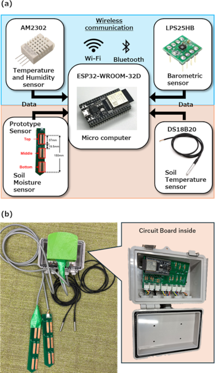
Fig. 1. (a) Conceptual diagram of the environmental measurement module composed of selected generic sensors. (b) External view of the prototype environmental measurement module.
1.4. Concept and Design of the Field Measurement Module
The developed field environmental measurement module is illustrated in Fig. 1. The system was constructed using the following components: DS18B20 sensor for soil temperature sensing, AM2302 sensor for air temperature and humidity, LPS25HB sensor for atmospheric pressure, and PVSS-03 sensor for solar radiation measurements. The PVSS-03 sensor was specifically selected for solar radiation. We implemented a prototype of the proposed three-point soil moisture sensor for soil moisture measurements. The microcomputer chosen for data processing was the ESP32-DevKitC-32D, which is a wireless communication-capable ESP32-WROOM-32D development board. We developed a field measurement sensor module consisting of sensors that were easy to handle and affordable to procure, prioritizing the simplicity of user implementation. Although monitoring crop growth status was possible using image processing via cameras, this method was excluded from this study because of the large volume of data required for communication.
A sensor hub circuit board was designed and developed to facilitate connections between these sensors. The case and cables were specified to meet the IPX3 water resistance standards. Operational verification was conducted by spraying water for 5 min within the \(±60°\) range from the vertical, as defined by the IPX3 standard, and the module was confirmed to function normally.
2. Challenges in Measuring Water Uptake by Plant Root Systems and the Development of the Three-Point Soil Moisture Sensor
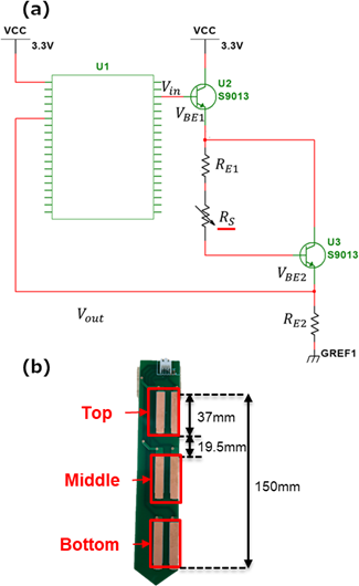
Fig. 2. (a) Circuit diagram for a single electrode of the three-point soil moisture sensor. (b) External view of the sensor.
2.1. Prototype Development of the Three-Point Soil Moisture Sensor
In this study, we focused on two issues inherent in conventional soil moisture sensors: (1) the structural limitation of only being installable at shallow depths, and (2) the sensors’ lack of spatial adaptability to align with critical root-zone water absorption points. We addressed this issue by developing a three-point soil moisture sensor (Fig. 2) with a structure designed to position the measurement electrodes at depths that physically corresponded to the plant root system. The aim of this design was to capture the moisture dynamics surrounding the root zone directly and objectively. This approach provides a foundational technology for acquiring the high-precision root zone data necessary for estimating water uptake model parameters, thereby contributing to the advancement of decision support systems and precision agriculture.
The sensor employs the electrical resistance method to ensure a low-cost realization in alignment with the DIO approach. The sensor measures the soil mass water content (\(u\)) by applying an electrical current to the soil and determining the resultant resistance. The sensor was inserted up to 150 mm below the surface, and the subsurface was divided into three layers at intervals of 19.5 mm. These layers were designated the lower layer (deepest point), top layer (shallowest point), and the middle layer (midpoint). Each layer had a measurement range of 37 mm and could be measured individually. The variable resistance \(R_s\) in the circuit represents the soil resistance, which fluctuates depending on the soil mass water content. Specifically, when \(u\) is high, the resistance decreases, whereas when \(u\) is low, the resistance increases. The relationship for \(u\) is expressed by Eq. \(\eqref{eq:moisture}\).
2.2. Calibration of the Multipoint Soil Moisture Sensor
To convert the output voltage (\(V_{\mathit{out}}\)) of the developed multipoint soil moisture sensor into volumetric water content (\(u\)), which is a standard metric in soil science, calibration experiments were conducted using soil collected from the experimental field. The objective of this experiment was to formulate the response characteristics of the sensor and enable the calculation of the observed values as the absolute water content, in compliance with standard methods. The experimental procedure is described as follows. First, the soil samples obtained from the university field were oven-dried at \(100° \text{C}\) for 60 min to create a reference sample with 0\(\%\) water content (complete dryness). Subsequently, water was added incrementally and uniformly mixed into the dry soil to prepare multiple samples with varying moisture conditions ranging from extreme aridity to saturation (0\(\%\) to approximately 40\(\%\)). Each sample was packed into a container at a constant pressure to replicate the bulk density of the field, followed by continuous measurement using the developed sensor. Immediately after each measurement, soil sub-samples were collected from the same containers to determine the true moisture content using a moisture analyzer (ML-50, A\(\&\)D Company, Ltd.). The ML-50 moisture analyzer is a high-precision instrument that directly calculates moisture content based on the “loss on drying method at \(105° \text{C}\),” which is a standard analytical technique derived from the weight change of the soil.
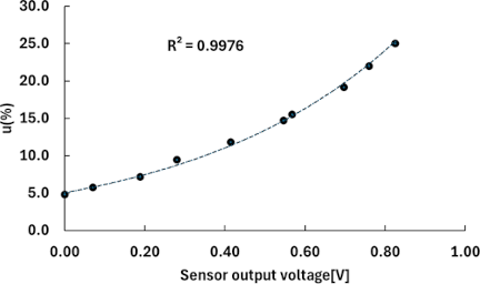
Fig. 3. Calibration curve for the proposed three-point soil moisture sensor relating the output voltage to the volumetric water content.
Analysis of the relationship between the sensor output and measured values revealed distinct nonlinearity. This is attributed to the synthesis of two physical and engineering factors. First, the electrical resistance of the soil, which is the target parameter of the resistive moisture sensor, is considered to decrease exponentially as conductive pathways are formed with increasing water content. Second, the output signal processed through the voltage conversion circuit of the sensor exhibits a nonlinear response. In this study, an exponential regression model was adopted using the output voltage as an explanatory variable and the volumetric water content as an objective variable. This model offers the practical advantage of enabling accurate moisture calculations, even on low-resource microcomputers typically deployed in agricultural fields. The calibration equation derived using the least-squares method is given by Eq. \(\eqref{eq:calibration}\).
Fig. 4. Conceptual diagram of the environmental monitoring system for broccoli growth in the field.
3. Analysis of Environmental Factors Influencing Crop Growth Based on Field Data Acquisition
3.1. Experimental Setup and Statistical Analysis
As shown in Fig. 4, sensor nodes were deployed in the experimental field plot. Environmental parameters, such as temperature, sensed by the subordinate nodes were transmitted to the master node via TCP/IP communication. Users can access the accumulated data using devices such as smartphones. Each subordinate node was equipped with eight sensors: an air temperature and humidity sensor, a solar radiation sensor, a barometric pressure sensor, a soil temperature sensor, and three-point soil moisture sensor (top, middle, and bottom layers). The sensor data were collected hourly. Hereinafter, the environmental data are defined as the air temperature (\(T_a\)), relative humidity (\(RH\)), integrated solar radiation (\(R_s\)), atmospheric pressure (\(P_a\)), soil moisture content (top: \(u_t\), middle: \(u_m\), bottom: \(u_b\)), soil temperature (\(T_s\)), and solar radiation (\(S\)). The crop growth metrics were collected manually on a daily basis.
Regression analysis was used to estimate the broccoli growth. Regression analysis is a statistical technique used to approximate the relationship between one set of variables (explanatory variables) and another set of variables (objective variables). In this study, the objective variables were the broccoli plant height and leaf count. The explanatory variables were the collected environmental data (\(T_a\), \(RH\), \(R_s\), \(P_a\), \(u_t\), \(u_m\), \(u_b\), \(T_s\), and \(S\)). Prior to regression analysis, the hourly collected environmental data were averaged to serve as the representative daily data. The process of fitting the objective variables using the explanatory variables based on the data collected during the experimental period, using the growth estimation model and regression analysis, is henceforth referred to as growth estimation. The goodness-of-fit of the model, specifically the growth estimation accuracy, was evaluated using the adjusted coefficient of determination (\(R^2\)). Hereinafter, the growth estimation accuracy is simply referred to as the estimation accuracy.
3.2. The Subject Crop
Fig. 5. (a) Cultivation of broccoli in the experimental field plot. (b) Measurement of the total plant height of broccoli after transplanting.
In this study, broccoli was the subject crop used for experimentation. Official Japanese policy stipulates that this crop will be registered as a vital vegetable by 2026. Statutory vegetables are defined as “vegetables of critical importance to the national livelihood” and include those with high or projected high consumption rates that are often managed under the Designated Vegetable Production Area System. Consequently, the agricultural value of broccoli is expected to increase significantly, driving the demand for advanced equipment in areas such as production and quality management. Although broccoli is a crop with relatively light harvests and low labor requirements, research has shown that insufficient soil moisture can lead to substantial reductions in both yield and quality 24. Crop growth and development are strongly dependent on meteorological factors such as temperature and solar radiation 11. Therefore, broccoli was determined to be a suitable crop for validating the efficacy of field environmental data monitoring and crop growth modeling. Fig. 5(a) illustrates the cultivation of broccoli in the experimental field plot and Fig. 5(b) shows the measurement of the total plant height following transplanting for growth documentation. Regression analysis, a method previously applied to other crops, was employed in this study for validation 25.
In this study, broccoli was cultivated within tunnel structures covered with insect-proof netting. To minimize interference with the microenvironment of the cultivation area, the measurement units and peripheral hardware were positioned outside the tunnels. Only the sensor probes were inserted beneath the netting and into the soil at the designated measurement points. Furthermore, because the tunnels were constructed using insect-proof netting, precipitation and solar radiation reached the soil surface without significant obstruction, although minor attenuation may have occurred. The field experiments were conducted in an experimental plot (15 m\(^2\)) located in Neyagawa, Osaka, Japan. A total of 32 broccoli plants (cv. Heiz SP) were transplanted on March 20, 2025. The soil at the experimental site was classified as Fluvisol with a predominantly clayey texture, reflecting the alluvial characteristics of the region. For environmental monitoring, sensor probes were installed at the center of each of the two cultivation rows within a 1.5 m \(\times\) 2.0 m area of the plot. This layout ensured that each probe was positioned symmetrically relative to the four broccoli plants in their respective rows, thus providing representative data of the rhizosphere environment. The sensors were placed at depths of 0–15 cm to capture the relevant soil moisture and temperature dynamics. The environmental data were collected at hourly intervals, and the 24 measurements per day were averaged to represent the daily values. The crop growth parameters were recorded once daily.
3.3. Analysis and Characterization of the Measured Environmental Data
Fig. 6. Comparison between the field environmental data (daily mean values) and the Japan Meteorological Agency data. (a) Daily mean soil water content across three depths (top, middle, and bottom layers), (b) daily mean atmospheric pressure and relative humidity, (c) daily mean air temperature and soil temperature, (d) daily integrated solar radiation, and (e) air temperature, precipitation, and solar radiation published by the Japan Meteorological Agency.
The field environmental data measured using the environmental monitoring module are presented in Figs. 6(a)–(d). For comparison, the air temperature, precipitation, and solar radiation data from the Japan Meteorological Agency for a city near the experimental field are shown in Fig. 6(e). The data were collected from March 22 to April 30, 2025, and the hourly measurements were averaged.
In this analysis, the temporal interaction with general weather conditions was evaluated using the time-series data from the field, as illustrated in Figs. 6(a)–(d). Fig. 6(a) shows the soil water content (top, middle, and bottom layers) measured using the three-point soil moisture sensor. Fig. 6(b) shows the temporal variations in the atmospheric humidity and atmospheric pressure, and Fig. 6(c) shows the variations in the air temperature and soil temperature. Collectively, these data comprehensively elucidated the effects of changing weather conditions on various soil properties within the experimental plot.
Figure 6(a) clearly revealed the influence of rainfall on soil moisture infiltration. During rainfall events, the water content of the surface layers (top and middle layers) increased sharply. This increase subsequently impacted the deeper layer (bottom layer) with a discernible time lag, resulting in elevated water content. This delay suggests that the soil possesses both high hydrophobicity in the top layer and high water retention capacity in the middle and bottom layers, indicating a staged progression of water infiltration from the surface to the interior. Conversely, during clear weather periods, the difference in water content between the middle and bottom soil layers was minimal, indicating a relatively uniform moisture distribution. Furthermore, the tendency of the bottom soil layer to exhibit higher water content than the middle layer was likely attributable to the ridge height of the experimental plot, which was approximately 10 cm. This structural configuration suggests that the middle layer, located approximately 10 cm below the surface, has enhanced aeration, whereas the bottom layer, situated approximately 15 cm below the surface, retains moisture more effectively.
Figures 6(b)–(d) capture the influence of external meteorological conditions on the internal soil environment. During rainy periods, an increase in atmospheric humidity and a concomitant decrease in atmospheric pressure and integrated solar radiation were observed. Furthermore, the daily integrated solar radiation, air temperature, and soil temperature fluctuated in a manner similar to that of the data provided by the Japan Meteorological Agency. This suggests that the measurement system accurately captures the changes in the external environment. Specifically, Fig. 6(b) illustrates the temporal variations in the humidity and atmospheric pressure, Fig. 6(c) shows the variations in the air and soil temperatures, and Fig. 6(d) shows the fluctuations in the solar radiation. We confirmed that there were strong correlations between these environmental parameters.
These analyses confirmed that the data acquired in this study fluctuated in a manner similar to that of the publicly available data from the Japan Meteorological Agency. Specifically, the soil water content data proved effective for a detailed examination of the water infiltration process into the soil matrix following rainfall, as well as the influence of the ridging structure on soil aeration and water retention capacity. These findings provide crucial foundational information for the optimization of water management and overall soil environmental conditions in the field plot.
4. Crop Growth Prediction Models Using Environmental Data
4.1. System Characterization and Research Objective
Data collection was conducted on open-field cultivated broccoli in an experimental field plot located on a university campus in Osaka Prefecture, Japan. The data acquisition period spanned approximately one month of the initial growth phase, from March 22 to April 30, 2025, following transplanting. In this study, we focused on estimating the growth of open-field broccoli. We defined multiple environmental factors that were expected to influence broccoli growth as the explanatory variables. These variables were the air temperature, relative humidity, atmospheric pressure, soil volumetric water content (top, middle, and bottom layers), solar radiation, and soil temperature, which were measured using a field measurement module that implemented generic sensors and a specialized three-point sensor for measuring the soil moisture at three depths. The objective variables were the daily measurements of broccoli plant height (PH) and leaf count (\(L_n\)).
Subsequently, we optimized these parameters to determine the growth estimation accuracy. The results would clarify the effects of applying the sensor module described herein and the benefits of introducing the three-point moisture sensor by comparing the characteristics of the proposed method with conventional approaches, ultimately revealing the optimal parameter settings for improving the growth estimation accuracy. For the evaluation, statistical and multiple regression analyses of the proposed growth estimation model were carried out using Python (3.12.11). The pandas (2.2.2) and scikit-learn (1.6.1) libraries were used for the analyses. All the analysis scripts were executed under identical conditions to confirm the reproducibility of the results.
4.2. Analysis Methodology
A model was constructed using multiple regression analysis as the primary analysis methodology. To explain and predict the objective variable, designated as growth (\(R\)), which represents the growth status of broccoli, based on multiple environmental factors (explanatory variables), we implemented multiple regression analysis, which is a widely used multivariate analytical technique. The model used for the multiple regression analysis is expressed by Eq. \(\eqref{eq:regression}\):
In multiple regression analysis, a problem known as multicollinearity arises when a high correlation exists between the explanatory variables, leading to unstable estimates of the regression coefficients. To address this issue, the variance inflation factor (VIF) was calculated to assess the presence of multicollinearity.
Table 2. Regression analysis results (coefficients and VIF).

The VIF serves as an indicator of the extent to which the variance of a regression coefficient for a specific explanatory variable is inflated due to its correlation with the other explanatory variables in the multiple regression model. The VIF value was calculated using Eq. \(\eqref{eq:vif}\):
The results after the exclusion of soil temperature (\(T_s\)) are presented in Table 3. The VIFs for all remaining explanatory variables were found to be low, where all of the values were less than 2. This signified a negligible correlation between the predictor variables, indicating that the estimation of the regression coefficients was highly stable. Consequently, the effect of multicollinearity on the model estimation was deemed insignificant. Furthermore, the coefficient of determination (\(R^2\)) were high for this revised model, where \(R^2=0.96\) for PH and \(R^2=0.94\) for leaf count (\(L_n\)).
Table 3. Revised regression analysis results (excluding soil temperature \(T_s\)).

This regression equation elucidated the magnitude and direction of the influence of each explanatory variable on broccoli growth. For instance, the positive coefficient for atmospheric pressure (\(P_a\)) (0.116) indicated a tendency for growth to increase when the atmospheric pressure was high, assuming that all other variables remained constant. Conversely, the negative coefficient for the top soil water content (\(u_t\)) (\(-1.059\)) indicated that the higher soil water content in the top layer led to reduced growth when other variables were constant. In this section, we constructed a multiple regression model after excluding soil temperature to circumvent multicollinearity. The resulting regression equation enabled the prediction of broccoli growth based on multiple environmental factors. Moving forward, it is essential to evaluate the fitness of the model using empirical data and validate its adequacy. Furthermore, a critical task would be to examine the causality of the sign and magnitude of each variable’s coefficient from a plant physiological perspective.
4.3. Contribution of Each Parameter to Crop Growth Estimation
In this study, the contribution of each explanatory variable to the crop growth estimation within the multiple regression model was evaluated (Table 4). First, when integrated solar radiation (\(S\)) was excluded from the model, the coefficient of determination (\(R^2\)) significantly dropped to 0.54. This clearly indicated that \(S\) was the dominant factor contributing to crop growth. Next, using the model from which \(S\) was already excluded, we estimated the PH by limiting the soil moisture sensor input to only one of the probes (top, middle, or bottom layer). The estimation results using a single probe yielded \(R^2\) values of 0.26, 0.32, and 0.25, respectively, showing no statistically significant difference based on probe depth. This single-probe estimation scenario corresponds to the use of a conventional, commercially available sensor that measures the soil moisture at only a single point and depth. However, throughout the measurement period, significant discrepancies were observed in the moisture values between the three probes used at different depths in this study, suggesting the complexity of the vertical gradient and distribution of water in the soil. The fact that single-depth measurements showed no difference in the prediction accuracy despite the large observed discrepancies between the probes strongly suggests that the simultaneous use of three measurement points at different depths allows the model to capture environmental factors that cannot be captured by single-depth measurements, thereby improving the growth estimation accuracy. This result provides critical insight that demonstrates the superiority of multipoint measurements.
Next, we compared the results of the PH estimation using a combination of two measurement points from the three soil moisture probes. The \(R^2\) values for the combinations of top and middle (\(u_t\)–\(u_m\)), middle and bottom (\(u_m\)–\(u_b\)), and top and bottom (\(u_t\)–\(u_b\)) were 0.48, 0.40, and 0.32, respectively. Among these, the top and middle combination (\(u_t\)–\(u_m\)) yielded the highest \(R^2\) value (0.48), maintaining approximately 90% of the explanatory power compared with the full three-point model (\(R^2=0.54\)). This outcome is highly relevant to the structure of the planted ridge and sensor placement. In this experiment, the ridge height was 10 cm, where the top probe (\(u_t\)) measured the moisture 5 cm below the ridge surface, and the middle probe (\(u_m\)) measured the moisture at the central core of the ridge. The high estimation accuracy achieved by the \(u_t\)–\(u_m\) combination suggests the significance of ensuring that irrigation adequately reaches not only the visible surface (\(u_t\)) but also the middle core of the ridge (\(u_m\)), where the primary root zone of the crop is likely to be situated. Conversely, conventional commercially available moisture sensors typically measure moisture near the ridge surface (corresponding to \(u_t\)). Our analysis indicates that measurements at a single shallow depth alone are insufficient to provide adequate information for accurate growth estimation. Instead, multilayered measurements, specifically those that include the middle core of the ridge, are indispensable. This result strongly implies the necessity for comprehensive, multipoint moisture data for robust growth modeling.
Table 4. Changes in the coefficient of determination (\(R^2\)) based on explanatory variable selection for PH estimation.

4.4. Evaluation of the Parameter Contributions using Standardized Coefficients
Although the regression models developed in the previous section demonstrated high estimation accuracy, the coefficients for each explanatory variable are based on diverse units, such as integrated solar radiation (\(S\)) and soil moisture (\(u\)). Consequently, it was difficult to directly compare the relative effects of each factor on crop growth. In this section, all explanatory variables were normalized to a mean of zero and variance of one to calculate the standardized regression coefficients (\(\beta^*\)), thereby statistically evaluating the contribution of each factor within the model.
The results of this analysis are summarized in Table 5. It can be seen that the integrated solar radiation (\(S\)) exhibited the largest positive contribution to PH. Regarding soil moisture (\(u\)), the results revealed distinct behaviors at different depths. Specifically, the soil moisture in the middle layer (\(u_m\): 10 cm depth) showed the second-highest positive contribution to PH after integrated solar radiation. This indicated that the moisture environment around a depth of 10 cm, where the primary rhizosphere was located, had a direct influence on vertical cell elongation in the broccoli. Among the soil moisture parameters, \(u_m\) was the most significant contributor. These findings suggest that multipoint sensing across different layers is more effective than single-depth measurements for identifying subtle differences in growth drivers. This is consistent with previous studies reporting that more than half of the root distribution in many crops is concentrated in the topsoil (approximately 8–20 cm) 26. Furthermore, in crops such as barley and maize, the water uptake rate per unit root length is higher in shallow layers (e.g., 0–15 cm) than in deeper layers 27. It has also been reported that the depth at which roots are most densely distributed is more critical than the maximum rooting depth for enhancing adaptation to water stress, and that the formation of such a dense root layer within the top 30 cm significantly promotes drought adaptation 28. Our results strongly support the efficacy of multipoint soil moisture monitoring for capturing these dynamics.
Table 5. Comparison of parameter contributions to PH based on standardized coefficients.

4.5. Results and Discussion
In this study, we developed a broccoli growth estimation model using an integrated monitoring system that combined low-cost environmental sensors with a customized multipoint soil moisture sensor. The resultant multiple regression model for PH demonstrated high precision, with a coefficient of determination (\(R^2\)) of 0.96. This result confirmed that crop growth was governed by the interactions between integrated solar radiation, which acted as the primary energy source, and vertical, multilayered soil moisture dynamics, which served as the physiological foundation. We concluded that such a high estimation accuracy was achieved by integrating both the photosynthetic energy from solar radiation and the rhizosphere moisture environment necessary to convert that energy into physical growth.
In this study, the proposed multipoint soil moisture sensor was measured at 5 cm intervals up to a depth of 15 cm. According to a previous study on broccoli root system development by Gherbin et al. 29, the root length density exhibited an extremely high value of 3.7 cm/cm\(^3\) in the topsoil layer (0–20 cm), whereas it decreased sharply to 0.8 cm/cm\(^3\) in the 40–60 cm layer. This suggests that water uptake and growth regulation activities are predominantly concentrated within a depth of 20 cm from the surface. In our model, we achieved a high accuracy in explaining growth variations using only moisture data up to a depth of 15 cm. This is likely attributable to the fact that this depth range, which contains the majority of the information necessary for growth prediction, constitutes the primary portion of the “active root zone.”
Furthermore, a previous study analyzing daily correlations of soil moisture at depths of 10, 20, and 40–120 cm using U.S. cropland data reported an extremely strong correlation (\(R^2 = 0.84\)) between the soil moisture in the surface layer (10 cm) and the immediately adjacent layer (20 cm) 30. This indicated that layers in close proximity (e.g., 20–30 cm and 30–40 cm) were highly correlated and operated synchronously without a significant time lag. By integrating our results with these findings, it can be argued that obtaining multilayered data up to a depth of 15 cm statistically covers the dynamics of the layers immediately beneath. Consequently, because deeper measurements may lead to information redundancy, we perceive that monitoring up to a depth of 15 cm is optimal in terms of balancing between estimation accuracy and practical feasibility.
With a compact depth configuration of 15 cm, the proposed system achieves a practical device design that does not interfere with agricultural operations, while maintaining high prediction accuracy. This identifies the optimal depth for acquiring growth-related information with minimal installation effort, contributing to the realization of efficient cultivation management and harvest prediction for smart agricultural irrigation support. Although the current model yielded high precision under uniform soil conditions in a small-scale plot, large-scale fields may require site-specific calibration to account for the spatial distribution of soil physical properties. This is an important subject for future research.
5. Conclusion
In this study, we addressed labor shortages resulting from an aging agricultural workforce by developing a low-cost environmental measurement module as part of an initiative to introduce smart agricultural technologies. Specifically, we investigated the relationships between environmental factors and broccoli growth, where broccoli was selected as the target crop. The experiment involved measuring and analyzing environmental data using a uniquely developed three-point soil moisture sensor and conventional general-purpose sensors. The results demonstrated that broccoli exhibited optimal growth within an air temperature range of 15°C–20°C. Furthermore, the multi-point setup successfully captured the details of the water infiltration process into the soil following rainfall. The evaluation and validation of the statistical model confirmed that the accuracy of growth prediction was highly dependent on the integrated solar radiation (\(S\)). Furthermore, enhancing the depth resolution of soil water content suggests the potential for improved complex factor estimation accuracy related to water absorption in broccoli growth. Although the current model achieved high precision in PH estimation under uniform soil conditions in a small-scale plot, large-scale fields may introduce spatial variability in the soil physical properties. This may necessitate site-specific calibration that considers the spatial distribution of soil characteristics, which remains an important subject for future research. Based on these insights, in future work, we intend to construct a refined growth prediction model that incorporates further investigations into the effective utilization of soil water content, air temperature, and solar radiation. Specifically, we aim to leverage the superiority of the multipoint soil moisture data to contribute to the optimization of irrigation and temperature management practices.
Acknowledgments
This work was supported by the Startup Research Grant from Osaka Electro-Communication University (OECU).
- [1] United Nations, Department of Economic and Social Affairs, “Population Division,” 2019.
- [2] E. Playán and L. Mateos, “Modernization and optimization of irrigation systems to increase water productivity,” Agricultural Water Management, Vol.80, pp. 100-116, 2006. https://doi.org/10.1016/j.agwat.2005.07.007
- [3] M. H. Ali and M. S. U Talukder, “Increasing water productivity in crop production – A synthesis,” Agricultural Water Management, Vol.95, pp. 1201-1213, 2008. https://doi.org/10.1016/j.agwat.2008.06.008
- [4] P. Debaeke and A. Aboudrare, “Adaptation of crop management to water-limited environments,” European J. of Agronomy, Vol.21, No.4, pp. 433-446, 2004. https://doi.org/10.1016/j.eja.2004.07.006
- [5] Z. Ahmed, D. Gui, G. Murtaza, L. Yunfei, and S. Ali, “An Overview of Smart Irrigation Management for Improving Water Productivity under Climate Change in Drylands,” Agronomy, Vol.13, Article No.2113, 2023. https://doi.org/10.3390/agronomy13082113
- [6] I. Tornese, A. Matera, M. Rashvand, and F. Genovese, “Use of Probes and Sensors in Agriculture-Current Trends and Future Prospects on Intelligent Monitoring of Soil Moisture and Nutrients,” AgriEngineering, Vol.6, No.4, pp. 4154-4181, 2024. https://doi.org/10.3390/agriengineering6040234
- [7] I. Lephondo, A. Telukdarie, I. Munien, U. Onkonkwo, and A. Vermeulen, “The Outcomes of Smart Irrigation System using Machine Learning to minimize water usage within the Agriculture Sector,” Procedia Computer Science, Vol.237, pp. 525-532, 2024. https://doi.org/10.1016/j.procs.2024.05.136
- [8] H. M. A. E. Baki, H. Fujimaki, I. Tokumoto, and T. Saito, “Optimization of irrigation scheduling using crop-water simulation, water pricing, and quantitative weather forecasts,” Frontiers in Agronomy, Vol.6, Article No.1376231, 2024. https://doi.org/10.3389/fagro.2024.1376231
- [9] B. Nsoh, A. Katimbo, H. Guo, D. M. Heeren, H. N. Nakabuye, X. Qiao, Y. Ge, D. R. Rudnick, J. Wanyama, E. Bwambale, and S. Kiraga, “Internet of Things-Based Automated Solutions Utilizing Machine Learning for Smart and Real-Time Irrigation Management: A Review,” Sensors, Vol.24, No.23, Article No.7480, 2024. https://doi.org/10.3390/s24237480
- [10] Y. Zhao, G. Li, S. Li, Y. Luo, and Y. Bai, “A Review on the Optimization of Irrigation Schedules for Farmlands Based on a Simulation-Optimization Model,” Water, Vol.16, No.17, Article No.2545, 2024. https://doi.org/10.3390/w16172545
- [11] M. Ohishi, M. Takahashi, M. Fukuda, and F. Sato, “Developing a Growth Model to Predict Dry Matter Production in Broccoli (Brassica oleracea L. var. italica) ‘Ohayou’,” The Horticulture J., Vol.92, No.1, pp. 77-87, 2023. https://doi.org/10.2503/hortj.QH-022
- [12] S. Yamazaki, Y. Kiriiwa, and M. Aono, “Estimation Evaluation of Strawberry Harvest Based on Regression Analysis with Integrated and Different Values,” The Institute of Electronics, Information and Communication Engineers,” Vol.J101-D, No.10, pp. 1466-1470, 2018.
- [13] B. Petrović, R. Bumbálek, T. Zoubek, R. Kuneš, L. Smutný, and P. Bartoš, “Application of precision agriculture technologies in Central Europe-review,” J. of Agriculture and Food Research, Vol.15, Article No.101048, 2024. https://doi.org/10.1016/j.jafr.2024.101048
- [14] M. Raj and M. Prahadeeswaran, “Revolutionizing agriculture: a review of smart farming technologies for a sustainable future,” Discover Applied Sciences, Vol.7, Article No.937, 2025. https://doi.org/10.1007/s42452-025-07561-6
- [15] C. J. Bryant, G. D. Spencer, D. M. Gholson, M. T. Plumblee, D. M. Dodds, G. R. Oakley, D. Z. Reynolds, and L. J. Krutz, “Development of a soil moisture sensor-based irrigation scheduling program for the Midsouthern United States,” Crop Forage Turfgrass Management, Vol.9, No.1, Article No.e20217, 2023. https://doi.org/10.1002/cft2.20217
- [16] V. Kumar, K. V. Sharma, N. Kedam, A. Patel, T. R. Kate, and U. Rathnayake, “A comprehensive review on smart and sustainable agriculture using IoT technologies,” Smart Agricultural Technology, Vol.8, Article No.100487, 2024. https://doi.org/10.1016/j.atech.2024.100487
- [17] T. Okayama, “Recommendation for Promoting Smart Agriculture Using Low-Cost Open Source Hardware,” Japanese J. of Farm Work Research, Vol.55, No.3, pp. 169-172, 2020. https://doi.org/10.4035/jsfwr.55.169
- [18] J. van de Gevel, J. van Etten, and S. Deterding, “Citizen science breathes new life into participatory agricultural research. A review,” Agronomy for Sustainable Development, Vol.40, Article No.35, 2020. https://doi.org/10.1007/s13593-020-00636-1
- [19] A. Z. Bayih, J. Morales, Y. Assabie, and R. A. de By, “Utilization of Internet of Things and Wireless Sensor Networks for Sustainable Smallholder Agriculture,” Sensors, Vol.22, No.9, Article No.3273, 2022. https://doi.org/10.3390/s22093273
- [20] C. Corbari, N. Paciolla, I. B. Charfi, D. Skokovic, J. A. Sobrino, and M. Woods, “Citizen science supporting agricultural monitoring with hundreds of low-cost sensors in comparison to remote sensing data,” European J. of Remote Sensing, Vol.55, No.1, pp. 388-408, 2022. https://doi.org/10.1080/22797254.2022.2084643
- [21] P. Taechatanasat and L. Armstrong, “Decision Support System Data for Farmer Decision Making,” Proc. of Asian Federation for Information Technology in Agriculture, pp. 472-486, 2014.
- [22] D. C. Rose and T. J. A. Bruce, “Finding the right connection: what makes a successful decision support system?,” Food Energy Secur., Vol.7, No.1, 2017. https://doi.org/10.1002/fes3.123
- [23] K. Momii, J. Nozaka, and T. Yano, “Comparison of root water uptake models,” J. of Japan Society of Hydrology and Water Resources, Vol.5, No.3, pp. 13-21, 1992. https://doi.org/10.3178/jjshwr.5.3_13
- [24] D. M. El-Shikha, P. Waller, D. Hunsaker, T. Clarke, and E. Barnes, “Ground-based remote sensing for assessing water and nitrogen status of broccoli,” Agricultural Water Management, Vol.92, No.3, pp. 183-193, 2007. https://doi.org/10.1016/j.agwat.2007.05.020
- [25] S. Yamazaki, Y. Kiriiwa, Nonmember, and M. Aono, “Estimation Evaluation of Strawberry Harvest Based on Regression Analysis with Integrated and Different Values,” IEICE Trans. on Information and Systems, Vol.J101-D, No.10, pp. 1466-1470, 2018.
- [26] J. Fan, B. McConkey, H. Wang, and H. Janzen, “Root distribution by depth for temperate agricultural crops,” Field Crops Research, Vol.189, pp. 68-74, 2016. https://doi.org/10.1016/j.fcr.2016.02.013
- [27] Y. Müllers, J. A. Postma, H. Poorter, J. Kochs, D. Pflugfelder, U. Schurr, and D. van Dusschoten, “Shallow roots of different crops have greater water uptake rates per unit length than deep roots in well‑watered soil,” Plant and Soil, Vol.481, pp. 475-493, 2022. https://doi.org/10.1007/s11104-022-05650-8
- [28] G.-R. Yu, J. Zhuang, K. Nakayama, and Y. Jin, “Root water uptake and profile soil water as affected by vertical root distribution,” Plant Ecology, Vol.189, No.1, pp. 15-30, 2007. https://doi.org/10.1007/s11258-006-9163-y
- [29] P. Gherbin, V. Miccolis, and V. Candido, “Root length density and yield traits of broccoli (Brassica oleracea L. var. italica Plenck) as affected by different techniques of seedling growing and transplanting,” Acta Horticulturae, Vol.1005, No.1005, pp. 427-434, 2013. https://doi.org/10.17660/ActaHortic.2013.1005.51
- [30] N. Li, T. H. Skaggs, P. Ellegaard, A. Bernal, and E. Scudiero, “Relationships among soil moisture at various depths under diverse climate, land cover and soil texture,” Science of the Total Environment, Vol.947, Article No.174583, 2024. https://doi.org/10.1016/j.scitotenv.2024.174583
- [a] Ministry of Agriculture, Forestry and Fisheries, “Smart Agriculture.” https://www.maff.go.jp/e/policies/tech_res/smaagri/robot.html [Accessed October 4, 2025]
- [b] WAGRI. https://wagri.naro.go.jp/ [Accessed October 4, 2025]
- [c] IPM Decisions (Integrated Pest Management). https://www.ipmdecisions.net/ [Accessed October 4, 2025]
- [d] Farm Cloud. https://farmcloud.eu/en/farmportal [Accessed October 4, 2025]
This article is published under a Creative Commons Attribution-NoDerivatives 4.0 Internationa License.