Paper:
LiDAR–Camera Fusion for 3D Fruit Counting and Density Mapping in Horizontal Trellis Orchards
Jaehwan Lee, Meguna Ohata, Hiromichi Itoh, and Eiji Morimoto

Graduate School of Agricultural Science, Kobe University
1-1 Rokkodai-cho, Nada-ku, Kobe, Hyogo 657-8501, Japan

This study presents a real-time fruit monitoring system that integrates light detection and ranging (LiDAR) and RGB camera data for 3D fruit counting and spatial density mapping in horizontal trellis pear orchards. The system employs instance-level sensor fusion, combining YOLO-based 2D fruit detection with SLAM-generated 3D point clouds to localize and track individual fruits. A customized temporal tracking algorithm mitigates duplicate counts, while center-based spatial filtering improves detection accuracy. Among the four evaluated YOLO models, YOLOv11s was selected based on its F1-score, lowest false negatives (FN) count, and real-time performance. Field validation in a 6 m × 70 m orchard plot demonstrated high counting accuracy (96.2%) and reliable spatial density estimation, with a mean absolute error of 0.64 fruits/m2. The system effectively identified yield variations across different orchard regions. These findings support the use of LiDAR–camera fusion for scalable, high-precision fruit monitoring in orchard environments, particularly in labor-intensive horizontal trellis systems.
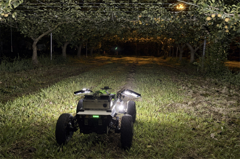
UGV with LiDAR-camera fusion system
1. Introduction
Recently, Japan’s agricultural sector has undergone significant structural transformations driven by demographic changes. According to the Ministry of Agriculture, Forestry and Fisheries (MAFF), the number of agricultural management entities has declined by approximately 22%, from 1.377 million in 2015 to 1.076 million in 2020 a,b. Additionally, the proportion of farmers aged 70 years and older has markedly increased from 26.8% to 51.0% over the same period.
This downward trend is also reflected in Japanese pear cultivation, where the bearing area decreased by approximately 23% between 2015 and 2024 c,d. This shrinking cultivation area poses a systemic threat to the industry, exacerbated by the labor-intensive nature of Japanese pear (Pyrus pyrifolia Nakai) production. On average, the crop demands approximately 380 labor hours per 10 ares, which is significantly more than that for deciduous fruits 1. This high labor requirement stems largely from meticulous fruit load management practices such as flower and fruit thinning, which are essential for balancing total yield with individual fruit quality 2.
These logistical challenges are intensified by the widespread use of horizontal trellis training systems. Although planar canopy structures are designed to optimize yield and fruit size, they require extensive pruning and branch training over large areas 3. In this context, traditional yield-monitoring methods remain a critical bottleneck. Manual visual inspections are not only time-consuming and labor-intensive but are also susceptible to human error 4,5. These inefficiencies render conventional practices increasingly unsustainable, highlighting the urgent need for automated systems capable of accurate spatial mapping and fruit counting to optimize labor deployment and enhance productivity.
In response to these challenges, the MAFF’s Promotion of Smart Agriculture report notes that while automated monitoring technologies have been widely adopted for land-extensive crops such as rice, fruit orchards face more complex structural constraints. To address this, the government has outlined a “Future Vision” that promotes the integration of robotic systems with optimized tree layouts to enable full automation. Government-led pilot trials have shown that technologies such as autonomous pesticide sprayers and transport units can reduce labor hours by approximately 60% to 80%, demonstrating the feasibility of unmanned operations in orchard environments e. Automated systems that utilize sensor technologies have been introduced to mitigate labor constraints 6. Periodic monitoring plays a vital role in precision fruit production, because accurate yield forecasting reduces the uncertainty in harvest volumes, enhances orchard management decisions, and supports more efficient regulation of shipment schedules 7. Recent developments in deep learning, particularly YOLO-series object detection models, have led to substantially advanced 2D image-based fruit detection. They achieve high accuracy and rapid inference speeds in diverse orchard environments by utilizing color, texture, and shape features to detect fruits under challenging conditions, including complex backgrounds, occlusion, and variable illumination 8. For example, YOLO-based models have demonstrated detection accuracies and inference speeds suitable for real-time deployment in orchard environments 9. However, 2D imaging lacks depth, which makes it insufficient for spatial mapping and individual fruit tracking. For instance, a small, nearby fruit and a large, distant fruit can generate identically sized 2D bounding boxes (bboxes). This depth ambiguity compromises critical functions: analysis of spatial relationships, quantification of yield distribution, and tracking of individual fruits.
To overcome this lack of depth information, LiDAR sensors have been integrated into agricultural robots to obtain high-precision 3D geometric data. Recent studies have demonstrated the applicability of LiDAR in agricultural environments. Kurashiki et al. confirmed its robustness for vehicle navigation over uneven agricultural terrain 10, while Shen et al. validated the feasibility of efficient motion estimation using sparse 3D point clouds 11. This data enables unmanned ground vehicle (UGV) systems to apply simultaneous localization and mapping (SLAM) technology, which generates consistent 3D maps while continuously tracking the robot’s position and orientation 12. However, spatial precision alone does not enable the identification of specific objects such as fruits. Point cloud data cannot distinguish between fruits, leaves, or branches because purely geometric methods lack semantic information. Therefore, combining the semantic detail of 2D imaging with the spatial accuracy of 3D data through sensor fusion is necessary.
Research on LiDAR–camera fusion has concentrated on two primary paradigms: point-level fusion, which processes entire point clouds at a high computational cost, and instance-level fusion, which selectively processes detected regions for improved efficiency 13,14. This selective approach enables modular operation and is well-suited for real-time applications.
Recent agricultural studies have shown the effectiveness of instance-level fusion in fruit detection and robotics applications. For example, Kurita et al. developed a sensor fusion system utilizing RGB cameras and LiDAR for autonomous navigation, thereby achieving accurate tree trunk recognition for self-localization in pear and apple orchards 15. Kang et al. demonstrated that accurate apple localization could be achieved in vertically trellised orchards using solid-state LiDAR–camera fusion with instance segmentation, showing improved robustness under intense sunlight compared with conventional stereo depth cameras 16.
However, existing research has primarily focused on vertically structured canopies, such as V-trellis systems. Few studies have explored the unique challenges posed by horizontal trellis systems, which are standard in Japanese pear cultivation. In such orchards, the wide spacing between trees requires multiple passes of UGVs to cover the entire plot. Under these conditions, conventional frame-to-frame 2D tracking struggles to maintain fruit identities, particularly during turns or loopbacks, which leads to significant duplicate counts. Moreover, preventing duplicate detections during continuous 3D spatial mapping and developing methods for quantitative fruit density visualization remain unresolved challenges.
This study proposes an environment-adaptive 3D monitoring framework specifically designed to address the geometric and operational constraints inherent to horizontal trellis orchards. We introduce two key technical innovations that extend beyond conventional monitoring methods.
First, to mitigate the instability of fruit localization caused by dynamic partial occlusion in upward-facing camera views, we propose a cumulative moving average (CMA)-based tracking filter. Unlike instantaneous detection, which can fluctuate owing to intermittent leaf occlusion, this method statistically stabilizes fruit centroid positions over time.
Second, to resolve the issue of duplicate counting inherent in multi-pass UGV traversals, we implement a global 3D instance management system. By anchoring fruit identities to absolute spatial coordinates—rather than relative image positions—this approach ensures consistent counting performance, regardless of the traversal complexity of the UGV.
2. Methodology
This section outlines the methodology of the proposed system for real-time 3D fruit counting and spatial mapping. Our approach uses a multimodal pipeline that fuses geometric LiDAR data with semantic RGB camera input. This design enables modularity and computational efficiency, while achieving real-time performance.
The methodology follows this structure: Section 2.1 describes the system architecture and intermodule data flow. Section 2.2 details the experimental platform and sensor configuration. Section 3 presents 2D fruit detection using YOLO. Section 4 describes the instance-level 3D localization and management. As shown in Fig. 1, the system architecture consists of two primary asynchronous modules: geometric mapping and semantic perception. These streams are fused at the instance level through a timestamp-based data association.
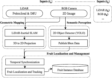
Fig. 1. System overview.
2.1. System Overview
The geometric-mapping module constructs a consistent 3D map. It uses FAST-LIO2 17, a LiDAR–inertial SLAM algorithm, to continuously generate a global 3D map and estimate the sensor’s six-degree-of-freedom pose. Concurrently, the Semantic Perception module provides situational awareness. It uses an optimized YOLO-based detector to identify fruit and locate them in 2D bboxes.
Because the geometric and semantic streams are generated independently, they must be aligned. A temporal synchronization step aligns the 3D map, sensor pose, and 2D detections using timestamps. The synchronized data is forwarded to the Fruit Localization and Management module. This module estimates the 3D position of each fruit and tracks its state and identity in the fruit instance database (FI-DB).
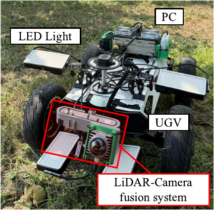
Fig. 2. The UGV experimental platform with LiDAR–camera sensor fusion system.
2.2. Experimental Platform
2.2.1. Hardware Configuration
As shown in Fig. 2, the experimental platform is a UGV (Hunter SE, AgileX Robotics). The UGV carries a custom perception system that integrates a LiDAR (Mid-360, Livox) and an RGB camera (ZED2i, Stereolabs) for sensor fusion.
Sensor placement was tailored to a Japanese pear orchard using a horizontal trellis training system. To capture overhead fruit, the RGB camera faced vertically upward, and the LiDAR was tilted by 26.5° to maximize the field of view overlap (Fig. 3(a)). However, the upward orientation caused significant sunlight-induced image saturation. The data acquisition strategy used to address this problem is described in Section 5.1. Data were logged on a dedicated computer (NUC11PAHi7, Intel). It ran ROS 2 (Humble) on Ubuntu 22.04 to record all sensor streams.
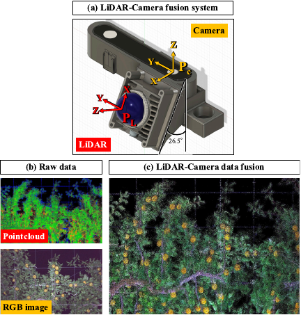
Fig. 3. The LiDAR–camera fusion system. (a) Sensor configuration. (b) Raw data showing manual correspondences between the RGB image and LiDAR point cloud. (c) The resulting dense, colored point cloud after calibration.
2.2.2. LiDAR–Camera Calibration
Accurate LiDAR–camera fusion requires a precise extrinsic transform \(\mathbf{T}_{\mathit{CL}}\). This matrix defines the rigid-body transformation that maps a 3D point \(\mathbf{p}_{3D,i}\) from the LiDAR coordinate system to its corresponding point \(\mathbf{p}_{2D,i}\) in the camera coordinate system.
As unstructured orchards degrade automatic calibration, we used the manual correspondence mode of the calibration toolbox 18. This process involved manually identifying a set of \(N\) corresponding point pairs \((\mathbf{p}_{3D,i}, \mathbf{p}_{2D,i})\) between the 3D point cloud and the 2D image (Fig. 3(b)).
Using these correspondences, the optimal matrix \(\mathbf{T}_{\mathit{CL}}^{\ast}\), is computed by solving the nonlinear least squares problem that minimizes the total re-projection error, as formulated in Eq. \(\eqref{eq:eq1}\).
3. 2D Fruit Detection
The Semantic Perception module identifies and localizes fruit in 2D RGB images. Developing a robust detector for this task requires a systematic approach, beginning with the construction of a custom dataset, followed by a structured process for model training and selection, and concluding with a clear definition of the evaluation metrics, as detailed in the following sections.
3.1. Dataset and Annotation
A custom dataset, foundational to the development of our perception model, was constructed using images acquired directly from the experimental site. To prepare the training data, each image was manually annotated using the LabelImg toolbox. During this process, every visible pear was enclosed in a bbox and assigned to a single “pear” class, as shown in Fig. 4. Following annotation, the complete dataset was partitioned into training, validation, and test subsets.
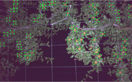
Fig. 4. Example of annotated pears in the dataset.
Table 1. Key hyperparameters for YOLO model training.

3.2. Model Training and Selection
This stage aimed to identify the optimal YOLO architecture for fruit detection. We trained four candidate models: YOLOv11n, YOLOv11s, YOLOv12n, and YOLOv12s 19,20.
All models were developed within the Ultralytics framework. We used transfer learning, initializing from COCO-pretrained weights to accelerate convergence. The key hyperparameters used in this process are listed in Table 1.
For a comprehensive performance evaluation, we used three standard metrics: Precision, Recall, and the F1-score. These metrics were derived from the model’s output on a test set, specifically by counting the number of true positives (TP), false positives (FP), and false negatives (FN).
Precision measures the accuracy of positive predictions (i.e., the proportion of detected boxes that correctly identified a fruit) and is calculated using Eq. \(\eqref{eq:eq3}\):
Recall measures the ability of the model to find all the actual fruits present in the images, as defined in Eq. \(\eqref{eq:eq4}\):
The F1-score is the harmonic mean of Precision and Recall, offering a single, balanced metric for overall performance, computed according to Eq. \(\eqref{eq:eq5}\):
To ensure the highest possible accuracy in yield estimation, our YOLO model selection strategy prioritizes the minimization of FNs. Initially, we used the F1-score to shortlist models with balanced precision and recall, but the decisive factor for the final selection was the model with the lowest FN rate. This approach is critical because, as previous studies have shown, missed fruits lead to persistent underestimation, particularly in dense and visually complex clusters 21. In contrast, FPs are less problematic because they can be reduced through post hoc filtering techniques such as temporal tracking and multi-view confirmation 22,23. Consequently, our strategy employed the F1-score as a preliminary screening metric, while the FN rate served as the primary selection criterion.
4. 3D Fruit Localization and Instance Management
The final stage of the pipeline is the localization and management of fruit instances in 3D space. This module receives synchronized data from the preceding modules to populate and maintain a global FI-DB. The internal workflow of this algorithm, as shown in Fig. 5, is detailed in the following sections.
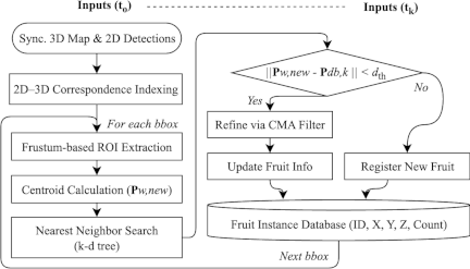
Fig. 5. Fruit localization and management algorithm.
4.1. 3D Fruit Instance Localization
This stage maps each 2D fruit detection to a 3D point \(\mathbf{p}_{W{\!\,},\mathit{new}}\), in the world coordinate frame. To achieve this, we project the relevant global 3D map onto the image using synchronized poses and calibration \((\mathbf{T}_{\mathit{CL}}, \mathbf{K})\). This pre-computation generates a pixel-to-point correspondence map, where each pixel \((u,v)\) maps to its associated 3D points in the world frame.
For each 2D detection, we isolated the relevant 3D points using the 2D bbox as a region of interest on the global point cloud. A frustum-based method extracts the corresponding point-cloud segment from each 2D detection. However, this initial cluster often contains significant background clutter from leaves and branches.
To remove clutter while preserving stable centroid estimation, we applied a spatial filter that retained only points projecting into the central 10% of the box. This central region filtering is motivated by center-based detection approaches 24,25. This design choice is dictated by the geometric constraints in the specific context of horizontal trellis systems. In an upward-facing camera configuration, a conventional 2D bounding box often includes background leaves situated at elevations higher than those of the target fruit. Consequently, averaging the depth values across the entire bounding box leads to a systematic overestimation of the fruit’s distance. To address this, the proposed method restricts depth estimation to the central 10% region of the bounding box. This focused sampling area is geometrically aligned with the convex, spherical surface of the pear, effectively excluding the flat background elements of the canopy and reducing depth estimation error. The final 3D position \(\mathbf{p}_{W{\!\,},\mathit{new}}\) is computed as the centroid of this refined point cluster.
4.2. Data Association
In horizontal trellis orchards, the wide spacing between trees requires the UGV to perform multiple passes and directional turns to fully observe the canopy. Under these conditions, relying solely on frame-to-frame 2D tracking proves inadequate, because fruits are frequently re-identified as new instances after the UGV executes a turn or loopback. To overcome this limitation, we implemented a global 3D instance management strategy. The detected fruits were associated based on their estimated 3D coordinates within the SLAM-generated map, enabling the system to maintain consistent fruit identities, regardless of the number or direction of observations. This approach effectively prevented duplicate counts during multi-pass operations.
To maintain a consistent track for each fruit over time, every new 3D observation \(\mathbf{p}_{W{\!\,},\mathit{new}}\), must be associated with an existing entry into the FI-DB. Each instance \(k\) is defined by its estimated 3D position \(\mathbf{p}_{\mathit{db},k}\), and its observation history.
The association process employs a nearest-neighbor search, accelerated by a k-d tree 26, to find the closest existing instance \(\mathbf{p}_{\mathit{db},k}\) to the new observation \(\mathbf{p}_{W{\!\,},\mathit{new}}\). A match is confirmed if the Euclidean distance between the two points is within a predefined distance threshold, \(d_{\mathit{th}}\), as defined in Eq. \(\eqref{eq:eq6}\).
The association search radius was set to \(d_{\mathit{th}} = 0.075\) m, considering that the transverse diameter of pear “Kousui” at harvest ranges from 83.2 mm to 95.1 mm. This threshold was established to balance two objectives: accommodating moderate localization uncertainty from SLAM drift and frustum-based projection, while preventing erroneous associations between spatially adjacent fruits by remaining smaller than the minimum fruit diameter.
4.3. Database and State Management
The FI-DB is a global data structure, maintained in-memory, that stores the state of each unique fruit instance observed by the system. The management of this database is dictated by the outcome of the data association step, which results in one of the following two scenarios:
-
1)
Successful association: If a new observation, \(\mathbf{p}_{W{\!\,},\mathit{new}}\), is successfully associated with an existing instance \(k\), then the state of that instance is updated. A CMA filter was applied to filter the measurement noise and refine its position estimate. CMA-based tracking is employed to accommodate the specific viewing conditions of the horizontal trellis system. Because the RGB camera captures fruit from a bottom-up perspective, the visual appearance of the fruit changes dynamically as the UGV moves. Leaves and branches frequently cause partial occlusions, resulting in a mixture of fruit and background within the bounding box. Consequently, the estimated fruit centroid may shift erratically, even for the same instance. When the UGV passes directly beneath a fruit, occlusion is temporarily reduced; however, it reappears as the viewing angle changes. The CMA functions as a temporal low-pass filter, smoothing out these geometric fluctuations across multiple observations. This filtering process allows the estimated centroid to gradually converge toward a stable position, thereby mitigating the instability caused by viewpoint variation. After the \(N_{k}\)-th observation of instance \(k\), its updated position, \(\mathbf{p}'_{\mathit{db},k}\), is calculated using Eq. \(\eqref{eq:eq7}\):
\begin{equation} \mathbf{p}'_{\mathit{db},k} = \dfrac{1}{N_k} \left\{\left(N_{k} - 1\right) \cdot \mathbf{p}_{\mathit{db},k} + \mathbf{p}_{W{\!\,},\mathit{new}}\right\}. \label{eq:eq7} \end{equation} -
2)
No association: If no association is found within the distance threshold, the observation is considered a previously unseen fruit. Consequently, a new instance is registered in the FI-DB with a unique ID, and its initial state is set using the current observation \(\mathbf{p}_{W{\!\,},\mathit{new}}\).
Finally, to ensure the reliability of the output by suppressing the transient FP, a confirmation filter is applied at the end of the process. Any fruit instance with a total observation count \(N_k\), does not meet a predefined minimum threshold, \(N_{\mathit{min}}\), is considered a spurious detection. Such unconfirmed instances are pruned from the FI-DB. The minimum observation threshold was set to \(N_{\mathit{min}} = 3\) to ensure that only fruits consistently detected across multiple observations are counted, thereby filtering out transient false detections while maintaining high recall for briefly visible fruits. The final output is the set of 3D positions of confirmed fruit instances.
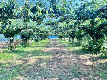
Fig. 6. The “horizontal trellis training system” cultivation environment of the Japanese pear orchard.
5. Experimental Setup
5.1. Experimental Site and Conditions
Field experiments were conducted on August 25, 2025, approximately one week before the anticipated harvest, in a Japanese pear orchard. The site, located at Kobe University’s Food Resources Education and Research Center, features pear trees trained on a horizontal trellis training system (Fig. 6), which was a key environmental factor guiding our data collection strategy. Data were collected from a single 6 m wide and 70 m long test plot. To ensure consistent image quality and mitigate issues related to natural lighting, all data acquisition was performed at night. The robotic platform was manually guided along the tree rows with LED panels providing controlled illumination of 725 lx at a measurement distance of 1.6 m from the camera.
5.2. Data Acquisition Protocol
We conducted data acquisition using a “stop-and-go” protocol, schematically shown in Fig. 7. The traversal path was planned to ensure comprehensive coverage of the 6 m \(\times\) 70 m experimental plot. Based on the LiDAR–camera fusion system’s 3 m horizontal field of view, the UGV followed a systematic bidirectional path with 1.5 m of lateral spacing between consecutive passes. This strategy resulted in a 1.5 m (50%) overlap region between adjacent passes, guaranteeing complete area coverage without data gaps.
At each acquisition point, the UGV advanced in 0.5 m increments and then remained stationary for a 5-second period. During this stationary phase, LiDAR point-cloud accumulation and RGB image acquisition for fruit detection were performed concurrently and synchronized using system timestamps. This stationary phase served two primary purposes. First, it allowed the Mid-360 LiDAR to accumulate a denser point cloud than would be possible from a single, continuous scan, thereby enhancing the fidelity of the geometric reconstruction. Second, this 5-second window provided ample time for the YOLO detection pipeline to process multiple image frames, enabling the generation of stable and reliable 2D bboxes for the subsequent sensor fusion stage.
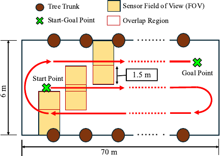
Fig. 7. Schematic of the data acquisition protocol in the experimental plot.
All sensor data were recorded in an ROS bag file. The RGB camera captured images at 2208 \(\times\) 1242-pixel resolution with an average frame rate of 8.3 fps. The complete dataset spanned approximately 100 minutes and contained 60,166 LiDAR scans (10 Hz), 1,203,302 IMU measurements (200 Hz), and 49,698 RGB images.
5.3. Evaluation Metrics and Procedure
The performance of the system was evaluated based on two primary objectives: aggregate counting accuracy and the accuracy of localized density estimation.
To assess the overall counting accuracy, the total number of confirmed fruit instances in the final FI-DB was compared with a manually annotated ground truth for the entire test plot. The total count error was then calculated to quantify the aggregate performance of the system in yield estimation.
To evaluate the accuracy of localized density Estimation, which assesses the system’s ability to capture spatial yield variations, the experimental plot was first divided into a grid of 2 m \(\times\) 2 m cells. The estimated fruit density [fruits/m\(^2\)] of each grid cell containing the ground-truth fruit instances was compared to the ground-truth density. Performance was quantified using the mean absolute error (MAE) to measure the magnitude of the estimation errors. The ground truth fruit positions were established using a manual annotation process. An annotator used the SLAM-generated colored point-cloud map as the primary canvas, overlaying it with synchronized video streams for validation. A unique 3D spatial marker was then placed at the center of each fruit, a method which inherently prevents any double-counting.
6. Experimental Results
This section presents the performance evaluation of the proposed system. First, the comparative results of the 2D fruit-detection models are presented to justify the selection of the optimal architecture. Subsequently, the overall performance of the complete 3D counting and spatial mapping pipeline is assessed using the field data.
Table 2. Summary of the dataset partitioning for model development and evaluation.

6.1. Performance of 2D Detection Models
The performance of the four candidate YOLO models was systematically evaluated to select the architecture that provides the optimal trade-off between detection accuracy and computational efficiency. This evaluation was conducted on a custom dataset constructed specifically for this study using images from the experimental site. To establish a standardized and reproducible workflow, the complete dataset was partitioned into training, validation, and test subsets. The detailed composition of each subset, including the number of images and “pear” annotations, is summarized in Table 2.
6.1.1. Model Training and Validation Performance
The training progress and validation performance of the four candidate models are presented in Fig. 8. The training and validation loss curves for all YOLO variants show stable convergence, indicating that all models were trained successfully. The initial quantitative evaluation was performed using a validation set. All models achieved high and tightly clustered mean average precision (mAP@0.5) scores ranging from 0.989 to 0.990. This instance level of performance is visually corroborated by the mAP curves, which rapidly saturate near the maximum value of 1.0. Furthermore, while the “Small” variants (YOLOv11s and YOLOv12s) reached a slightly higher F1-score of 0.970, the overall performance difference between the models was negligible. Given that neither the quantitative metrics nor the visual evidence from the training curves revealed a definitively superior model in this phase, a final evaluation on the test set was necessary for a definitive model selection.
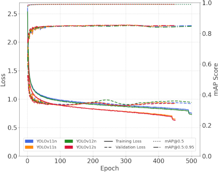
Fig. 8. Training curves for YOLO models.
Table 3. Performance summary of YOLO models on the test set.

6.1.2. Test-Set Evaluation and Model Selection
The final evaluation used the test set to measure the generalizability of each model. During this evaluation, a confidence threshold of 0.7 was applied to filter out low-confidence predictions. Table 3 shows that YOLOv11s had the highest F1-score (0.983), reflecting balanced results. Choosing the best model involves looking beyond the F1-score and analyzing the types of errors that occur. In agricultural yield estimation, it is especially important to minimize the FN because missing fruits leads to permanent yield loss. Although YOLOv12n had the highest precision of 0.984, it also had the highest number of FNs with 159 instances. In comparison, YOLOv11s had a higher recall (0.986) and only 55 FN. Because it combines a high F1-score with a low number of FN, YOLOv11s was chosen as the best 2D detector for this task. An inference time of 8.02 milliseconds also indicates that it can be used in real-time applications.
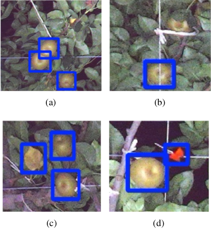
Fig. 9. Qualitative error analysis of YOLOv11s.
6.1.3. Error Analysis and Model Selection
A qualitative error analysis of the YOLOv11s predictions revealed that the detector was robust under challenging conditions, including clustered and partially occluded fruits, as shown in Figs. 9(a) and (b). The analysis revealed that FPs primarily stemmed from background objects mimicking pear-like features, such as senescent yellow leaves or red agricultural tape (Figs. 9(c) and (d)). FNs were most common in cases of severe occlusion or within low-illumination shadows where fruit features were indistinct.
For yield estimation, minimizing FNs is more critical, because the data association mechanism can filter out transient incorrect detections through repeated observations, whereas missed fruits lead to irreversible counting losses. Given its high F1-score (0.983), lowest FN count (55), and real-time inference speed (8.02 ms), YOLOv11s was selected as the optimal 2D detector for the final system.
6.2. System Performance on 3D Counting and Mapping
The overall system performance was evaluated by deploying the selected YOLOv11s model within the full 3D counting and spatial mapping pipeline. The following sections detail the quantitative and qualitative results of the data collected from the entire experimental plot.
6.2.1. Overall Counting Accuracy and Error Analysis
The aggregate counting accuracy of the system was evaluated by comparing the final estimated count with a manually annotated ground truth. The system estimated a total of 1,963 fruits compared with the ground truth of 1,891 fruits, yielding a net over-count of 72 fruits, corresponding to a relative counting error of 3.8% and an overall counting accuracy of 96.2%.
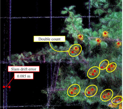
Fig. 10. Example of double counting caused by SLAM drift error.
A detailed error analysis showed that the system missed only 14 of the 1,891 ground-truth instances, resulting in a low miss rate of 0.7%. The net over-counting of 72 fruits was attributed to 86 FPs. These errors underscore the need for targeted mitigation strategies at two distinct stages of the process.
At the detection stage, 33 FPs were attributed to YOLO misclassifying yellow leaves and red tape as fruit. These errors can be mitigated by increasing the confidence threshold from 0.7 to suppress ambiguous detection, or by augmenting the training set with negative samples of senescent leaves and red agricultural tape.
In the localization stage, 53 instances of double-counting occurred despite the implementation of CMA filtering, which associates 2D detection results with 3D point-cloud data through temporal tracking (Section 4.3). Further analyses identified two primary causes. Thirty instances occurred within the association threshold (\(d_{\mathit{th}} = 0.075\) m), suggesting limitations in temporal filtering or in the precision of the k-d tree search algorithm. The remaining 23 instances resulted from localized SLAM drift that exceeded the association threshold, particularly during UGV turning maneuvers.
As illustrated in Fig. 10, a drift error of 0.085 m occurred during a turning maneuver. This drift prevented the system from recognizing that consecutive observations corresponded to the same fruit. Consequently, the CMA filtering mechanism generated a \(\mathbf{p}_{W{\!\,},\mathit{new}}\), leading to duplicate entries in the dataset. When the SLAM drift exceeded a defined threshold, the system assigned different IDs to the same physical fruit, resulting in multiple counts for a single object.
Although CMA filtering helps mitigate the localization uncertainty, significant SLAM drift during dynamic motion remains a persistent challenge. Incorporating loop closure constraints can reduce the cumulative drift during turning maneuvers, whereas proximity-based clustering applied in post-processing can merge duplicate detections caused by excessive drift. Implementing these strategies in future system deployments will enhance the robustness of the system and the overall localization accuracy.
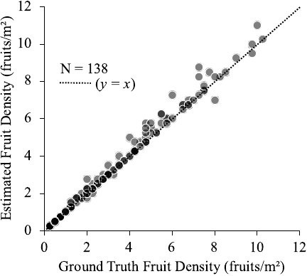
Fig. 11. Correlation scatter plot of fruit density.
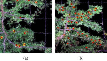
Fig. 12. 3D visualization of estimated fruit positions (red dots) in representative grid cells. (a) Sparse region: 2.5 fruits/m\(^2\). (b) Dense region: 10.25 fruits/m\(^2\).
6.2.2. Fruit Density Map with Spatial Localization
The system’s ability to capture spatial variation was evaluated by comparing the estimated and ground-truth fruit densities across 138 grid cells containing fruits. The quantitative results (Fig. 11) demonstrate strong agreement, with an MAE of 0.64 fruits/m\(^2\). This low error indicates consistent accuracy across a range of density conditions.
Visual confirmation is provided by 3D map visualizations (Fig. 12), where detected fruit locations are marked with red dots on the colored point cloud. Good performance is observed across all density ranges. Individual fruits are clearly identified in sparse regions (2.5 fruits/m\(^2\)), whereas clustered fruits are successfully distinguished in dense regions (10.25 fruits/m\(^2\)). These findings confirm that accurate fruit density maps are generated by the proposed method, capturing yield variations across the orchard.
The accurate identification of sparse regions using the density map serves as a valuable diagnostic tool for orchard management. Low-density areas may have issues such as poor tree vigor, localized disease, or inadequate pollination, which require targeted investigation. Furthermore, this spatial information provides data-driven evidence for canopy management. This enables farmers to use the map during winter pruning to make informed decisions regarding branch training, specifically to fill unproductive gaps. This practice optimizes sunlight interception and improves yield potential for the subsequent season.
7. Conclusion
This paper presented a LiDAR-RGB fusion system developed for 3D fruit counting and spatial density mapping in Japanese pear orchards using horizontal trellis training. For 2D fruit detection, we compared YOLO architectures and identified YOLOv11s as the optimal model, achieving an F1-score of 0.983 while minimizing the FNs critical for yield prediction. The integration of this detector with FAST-LIO2 SLAM enabled continuous 3D mapping across orchard scales. Field experiments involving 1,891 fruits validated the complete system. The system achieved a counting error of 3.8% and an MAE of 0.64 fruits/m\(^2\) for spatial density estimation.
Despite these promising results, the proposed method had some limitations. FPs from the 2D detector and double counting owing to SLAM drift remain the primary error sources.
Future work will focus on improving the training data and SLAM algorithms to enhance system robustness. Furthermore, we aim to extend the system toward spatio-temporal monitoring to track individual fruit growth throughout the growing season.
Acknowledgments
This work was supported by the JSPS Grant-in-Aid for Early-Career Scientists (Grant Number: 25K18327).
- [1] R. Imai, “Farm management characteristics and structural reorganization in deciduous fruit production,” J. of Rural Problems, Vol.21, No.4, pp. 183-189, 1985 (in Japanese). https://doi.org/10.7310/arfe1965.21.183
- [2] H. Hayama et al., “Early yield and fruit quality of Japanese pear ‘Hosui’ trained with a V-shaped trellis system,” Horticultural Research (Japan), Vol.22, No.1, pp. 55-61, 2023 (in Japanese). https://doi.org/10.2503/hrj.22.55
- [3] J. Gené-Mola et al., “Fruit detection and 3D location using instance segmentation neural networks and structure-from-motion photogrammetry,” Computers and Electronics in Agriculture, Vol.169, Article No.105165, 2020. https://doi.org/10.1016/j.compag.2019.105165
- [4] H. Mirhaji, M. Soleymani, A. Asakereh, and S. A. Mehdizadeh, “Fruit detection and load estimation of an orange orchard using the YOLO models through simple approaches in different imaging and illumination conditions,” Computers and Electronics in Agriculture, Vol.191, Article No.106533, 2021. https://doi.org/10.1016/j.compag.2021.106533
- [5] A. B. Payne, K. B. Walsh, P. P. Subedi, and D. Jarvis, “Estimation of mango crop yield using image analysis – Segmentation method,” Computers and Electronics in Agriculture, Vol.91, pp. 57-64, 2013. https://doi.org/10.1016/j.compag.2012.11.009
- [6] A. Koirala, K. B. Walsh, Z. Wang, and C. McCarthy, “Deep learning – Method overview and review of use for fruit detection and yield estimation,” Computers and Electronics in Agriculture, Vol.162, pp. 219-234, 2019. https://doi.org/10.1016/j.compag.2019.04.017
- [7] U.-O. Dorj, M. Lee, and S.-S. Yun, “An yield estimation in citrus orchards via fruit detection and counting using image processing,” Computers and Electronics in Agriculture, Vol.140, pp. 103-112, 2017. https://doi.org/10.1016/j.compag.2017.05.019
- [8] P. Chu, Z. Li, K. Lammers, R. Lu, and X. Liu, “Deep learning-based apple detection using a suppression mask R-CNN,” Pattern Recognition Letters, Vol.147, pp. 206-211, 2021. https://doi.org/10.1016/j.patrec.2021.04.022
- [9] R. Sapkota et al., “Comprehensive performance evaluation of YOLOv12, YOLO11, YOLOv10, YOLOv9 and YOLOv8 on detecting and counting fruitlet in complex orchard environments,” arXiv:2407.12040, 2024. https://doi.org/10.48550/arXiv.2407.12040
- [10] K. Kurashiki, K. Kono, and T. Fukao, “LiDAR based road detection and control for agricultural vehicles,” J. Robot. Mechatron., Vol.36, No.6, pp. 1516-1526, 2024. https://doi.org/10.20965/jrm.2024.p1516
- [11] S. Shen, T. Ito, and T. Hirose, “Spatio-temporal gradient flow for efficient motion estimation in sparse point clouds,” J. Robot. Mechatron., Vol.37, No.6, pp. 1327-1342, 2025. https://doi.org/10.20965/jrm.2025.p1327
- [12] T. Shan et al., “LIO-SAM: Tightly-coupled lidar inertial odometry via smoothing and mapping,” 2020 IEEE/RSJ Int. Conf. on Intelligent Robots and Systems, pp. 5135-5142, 2020. https://doi.org/10.1109/IROS45743.2020.9341176
- [13] S. Vora, A. H. Lang, B. Helou, and O. Beijbom, “PointPainting: Sequential fusion for 3D object detection,” 2020 IEEE/CVF Conf. on Computer Vision and Pattern Recognition, pp. 4603-4611, 2020. https://doi.org/10.1109/CVPR42600.2020.00466
- [14] C. R. Qi, W. Liu, C. Wu, H. Su, and L. J. Guibas, “Frustum PointNets for 3D object detection from RGB-D data,” 2018 IEEE Conf. on Computer Vision and Pattern Recognition, pp. 918-927, 2018. https://doi.org/10.1109/CVPR.2018.00102
- [15] H. Kurita, M. Oku, T. Nakamura, T. Yoshida, and T. Fukao, “Localization method using camera and LiDAR and its application to autonomous mowing in orchards,” J. Robot. Mechatron., Vol.34, No.4, pp. 877-886, 2022. https://doi.org/10.20965/jrm.2022.p0877
- [16] H. Kang, X. Wang, and C. Chen, “Accurate fruit localisation using high resolution LiDAR-camera fusion and instance segmentation,” Computers and Electronics in Agriculture, Vol.203, Article No.107450, 2022. https://doi.org/10.1016/j.compag.2022.107450
- [17] W. Xu, Y. Cai, D. He, J. Lin, and F. Zhang, “FAST-LIO2: Fast direct LiDAR-inertial odometry,” IEEE Trans. on Robotics, Vol.38, No.4, pp. 2053-2073, 2022. https://doi.org/10.1109/TRO.2022.3141876
- [18] K. Koide, S. Oishi, M. Yokozuka, and A. Banno, “General, single-shot, target-less, and automatic LiDAR-camera extrinsic calibration toolbox,” arXiv:2302.05094, 2023. https://doi.org/10.48550/arXiv.2302.05094
- [19] R. Khanam and M. Hussain, “YOLOv11: An overview of the key architectural enhancements,” arXiv:2410.17725, 2024. https://doi.org/10.48550/arXiv.2410.17725
- [20] Y. Tian, Q. Ye, and D. Doermann, “YOLOv12: Attention-centric real-time object detectors,” arXiv:2502.12524, 2025. https://doi.org/10.48550/arXiv.2502.12524
- [21] D. Xu et al., “Improving passion fruit yield estimation with multi-scale feature fusion and density-attention mechanisms in smart agriculture,” Computers and Electronics in Agriculture, Vol.239, Part A, Article No.110958, 2025. https://doi.org/10.1016/j.compag.2025.110958
- [22] S. Jin, L. Zhou, and H. Zhou, “CO-YOLO: A lightweight and efficient model for Camellia oleifera fruit object detection and posture determination,” Computers and Electronics in Agriculture, Vol.235, Article No.110394, 2025. https://doi.org/10.1016/j.compag.2025.110394
- [23] T. Yu, C. Hu, Y. Xie, J. Liu, and P. Li, “Mature pomegranate fruit detection and location combining improved F-PointNet with 3D point cloud clustering in orchard,” Computers and Electronics in Agriculture, Vol.200, Article No.107233, 2022. https://doi.org/10.1016/j.compag.2022.107233
- [24] T. Yin, X. Zhou, and P. Krähenbühl, “Center-based 3D object detection and tracking,” 2021 IEEE/CVF Conf. on Computer Vision and Pattern Recognition, pp. 11779-11788, 2021. https://doi.org/10.1109/CVPR46437.2021.01161
- [25] C. Xin, T. Motz, A. Hartel, and E. Kasneci, “OCDet: Object center detection via bounding box-aware heatmap prediction on edge devices with NPUs,” arXiv:2411.15653, 2024. https://doi.org/10.48550/arXiv.2411.15653
- [26] S. Shen, M. Saito, Y. Uzawa, and T. Ito, “Optimal clustering of point cloud by 2D-LiDAR using Kalman filter,” J. Robot. Mechatron., Vol.35, No.2, pp. 424-434, 2023. https://doi.org/10.20965/jrm.2023.p0424
- [a] Ministry of Agriculture, Forestry and Fisheries of Japan (MAFF), “2015 census of agriculture and forestry in Japan,” 2016 (in Japanese). https://www.e-stat.go.jp/stat-search/files?page=1&layout=datalist&toukei=00500209&tstat=000001032920&cycle=7&year=20150&month=0&tclass1=000001077437&tclass2=000001077396&tclass3=000001089555&tclass4val=0 [Accessed January 20, 2026]
- [b] MAFF, “2020 census of agriculture and forestry in Japan,” 2021 (in Japanese). https://www.e-stat.go.jp/stat-search/files?page=1&layout=datalist&toukei=00500209&tstat=000001032920&cycle=7&year=20200&month=0&tclass1=000001147146&tclass2=000001155386&tclass3=000001159186&tclass4val=0 [Accessed January 20, 2026]
- [c] MAFF, “2015 fruit production and shipment statistics,” 2016 (in Japanese). https://www.e-stat.go.jp/stat-search/files?page=1&toukei=00500215&tstat=000001013427&tclass1=000001032287&tclass2=000001032927&tclass3=000001088895 [Accessed January 20, 2026]
- [d] MAFF, “2024 fruit production and shipment statistics,” 2025 (in Japanese). https://www.e-stat.go.jp/stat-search/files?page=1&toukei=00500215&tstat=000001013427&tclass1=000001032287&tclass2=000001032927&tclass3=000001236584 [Accessed January 20, 2026]
- [e] MAFF, “Promotion of smart agriculture,” 2025. https://www.maff.go.jp/e/policies/tech_res/smaagri/PDF/Promotion_of_SmartAgriculture_250131.pdf [Accessed January 20, 2026]
This article is published under a Creative Commons Attribution-NoDerivatives 4.0 Internationa License.