Collision Detection of Small Paddy-Field Robots with Soft Obstacles Based on Wavelet Analysis of Estimated Collision Force

Kentaro Kameyama; Rikuto Iizuka

doi:10.20965/jrm.2026.p0439

single-rb.php

« previous

JRM Vol.38 No.2 pp. 439-448

(2026)

doi: 10.20965/jrm.2026.p0439

Paper:

Views over last 60 days: 6

Collision Detection of Small Paddy-Field Robots with Soft Obstacles Based on Wavelet Analysis of Estimated Collision Force

Kentaro Kameyama and Rikuto Iizuka

National Institute of Technology, Fukui College
Geshi, Sabae, Fukui 916-0029, Japan

Received:

September 15, 2025

Accepted:

January 24, 2026

Published:

April 20, 2026

Keywords:

field robot, agriculture robot, traveling irregular ground, collision detection, Kalman filter

Abstract

This study investigates a method for collision detection caused by soft and deformable obstacles, such as soil and plants (soft obstacles). Field robots must operate while interacting with the soft obstacles in their environments. However, previous studies on collision detection have primarily focused on hard obstacles, such as rocks and artificial structures, and research addressing soft obstacles has been limited. Because soft obstacles absorb impact forces, collision detection using conventional methods is challenging, and determining the collision time is even more difficult. To address these challenges, this study proposes a method that estimates the states, including unknown collision forces, using an extended Kalman filter. A wavelet transform is then applied to the estimated values to detect collisions. The effectiveness of the proposed method was validated using experimental data obtained from a water tank.

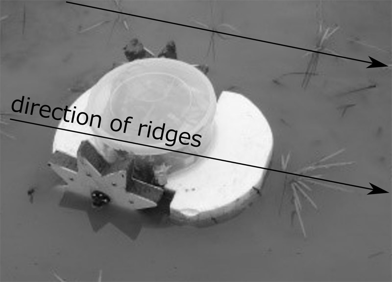
Example of stranding of a small paddy-field robot (riding over an underwater obstacle)

Close full text

Cite this article as:

K. Kameyama and R. Iizuka, “Collision Detection of Small Paddy-Field Robots with Soft Obstacles Based on Wavelet Analysis of Estimated Collision Force,” J. Robot. Mechatron., Vol.38 No.2, pp. 439-448, 2026.

Data files:

1. Introduction

Field robots, such as agricultural, disaster response, and environmental survey robots, have attracted significant attention in recent years. Furthermore, although conventional research has mainly focused on large- and medium-sized robots that automate existing robots, active studies are currently being conducted on small robots. For example, Seki et al. verified the weeding performance of a small robot equipped with a weeding brush and tactile sensors ^1,2,3. In addition, Maruyama and Naruse proposed a two-wheeled differential-drive robot ⁴, and Iwakabe et al. proposed a weeding robot equipped with an arm on a tracked vehicle ^5,6. Iwano et al. developed and evaluated a compact electrically driven flail-type mowing system that is designed to reduce the workload of agricultural mowing tasks, which could also be used on narrow paddy ridges ⁷. Although methods for utilizing the advantages of small robots have been explored, challenges remain. Small robots are easily affected by obstacles such as terrain and plants.

Numerous studies have reported collisions between robots and obstacles. For example, in ⁸, collisions of robotic arms were categorized into seven steps (pre-collision, detection, isolation, identification, classification, reaction, and post-collision), and the advantages and disadvantages of various collision detection methods were discussed. In studies targeting mobile robots, many approaches have been proposed to detect and avoid obstacles using non-contact sensors such as omnidirectional cameras and LiDAR ^9,10. Approaches that assume collisions have been proposed such as evaluating the vibrations of a robot bumper to distinguish grass from rocks ¹¹, and classifying acceleration data to detect collisions of small paddy-field robots with ridges ¹².

However, actual obstacles include not only hard objects but also soft and deformable ones, such as plants and ground irregularities (hereinafter referred to as “soft obstacles”). Because soft obstacles absorb collision energy, it is difficult for conventional methods to detect collisions, precisely. Furthermore, weeding robots may need to continue moving forward while pushing aside obstacles even after a collision. In this case, there is a risk of stranding by climbing over an obstacle, and it is necessary for the robots to determine whether to push through or avoid the obstacle.

To address this issue, one of the authors proposed a collision-detection method for a small paddy-field robot that collides with underwater obstacles as a model case ¹³. The proposed method estimates unknown collision forces from the acceleration data of the robot using an extended Kalman filter and detects collisions based on the estimated results. However, because the estimated collision forces contain oscillatory components, it is difficult to determine the collision time by relying solely on local estimates.

To solve this problem, this study proposes a method that applies a wavelet transform to the estimated values including the unknown collision force to estimate the collision time accurately. Moreover, in this approach, the mathematical model of the robot is refined to improve the estimation accuracy.

The remainder of this paper is organized as follows. Section 2 discusses the collection and interpretation of experimental data related to stranding. Section 3 describes the construction of the collision detector. Sections 3.1 and 3.2 formulate the mathematical model representing the robot behavior, and Section 3.3 explains the state estimation of the model, including unknown exogenous inputs. Section 3.4 presents a method for determining the collision time by applying wavelet transforms to the estimated values. Section 4 presents an evaluation of the effectiveness of the proposed method using experimental data. Finally, Section 5 provides the conclusions of this study. The linearization of the mathematical model and algorithm of the extended Kalman filter are included in the appendices.

2. Problem Statement

2.1. Collision of Robot with Soft Obstacles

An example of a robot being stranded during a field test is shown in Fig. 1. The robot used in this study is a small weeding robot for paddy fields developed by one of the authors ¹⁴. It is a two-wheeled vehicle equipped with balance floats at the front and rear of its body, and is designed for operation in flooded paddy fields.

As shown in Fig. 1, the robot rode up onto a ridge and could not move forward or backward. In this situation, the robot was still operable immediately after colliding with the ridge. However, by continuing to move forward after the collision, it mounted the ridge deeper and was unable to operate.

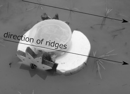
Fig. 1. Example of stranding of a small paddy-field robot (riding over an underwater obstacle).

A water-tank experiment was conducted to understand the behavior of the robot during the stranding process. The experimental setup is illustrated in Figs. 2 and 3.

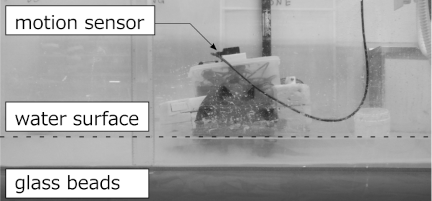
Fig. 2. Experimental setup for collision and stranding tests of a small-paddy field robot.

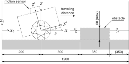
Fig. 3. Coordinate systems of the experimental robot and motion sensor.

The experimental water tank was made of acrylic and had dimensions of \(1200 \times 600 \times 600~\text{mm}\) (width \(\times\) depth \(\times\) height). The bottom of the tank was covered with a 50 mm layer of a glass bead mixture, which was used as a substitute for mud. The mixture consisted of glass beads with particle sizes of 38–53, 355–500, and 710–1000 μm (glass bead abrasive FGB-320, 40, 20, Fuji Manufacturing Co., Ltd.), mixed in a \(2:2:1\) ratio. This mixture ratio was selected to simulate actual paddy soil. In our previous study ¹⁵, evaluations via flat-plate sinking tests confirmed that this ratio exhibits physical responses (such as bearing capacity) similar to those of natural paddy fields.

The experimental robot was designed using the same concept as that used in the field tests, with dimensions of \(240 \times 365 \times 340~\text{mm}\) (width \(\times\) length \(\times\) height). The robot was equipped with star-shaped wheels with a diameter of 180 mm and a thickness of 25 mm, with each wheel featuring eight protrusions. Under a traveling load, the rotational speed of the wheels was approximately 10 rpm, resulting in a traveling speed of 100 mm/s. The track width was set to 140 mm (wider than the obstacle width). The total mass of the robot was 3.45 kg.

The expected water depth was 50 mm, providing a clearance of 20 mm between the bottom of the robot and ground.

The behavior of the robot was measured using a three-axis motion sensor (HWT905-TTL MPU-9250, WitMotion) mounted on the robot, which recorded the acceleration, angular velocity, angles, and magnetic field. The specifications of the sensor are listed in Table 1.

Table 1. Specifications of the three-axis motion sensor.

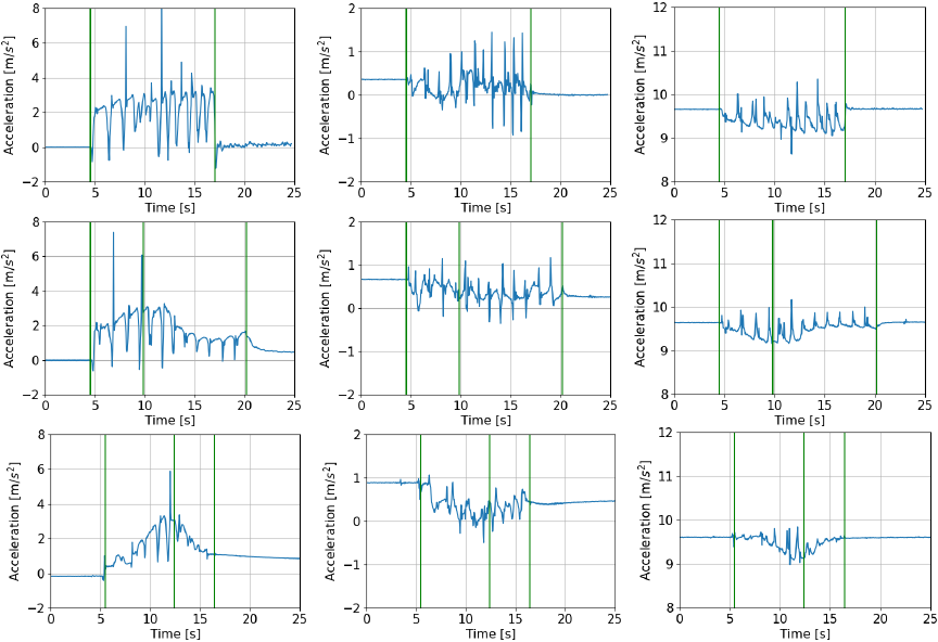
Fig. 4. Example of the measured acceleration (\(X\): left, \(Y\): center, \(Z\): right) for three obstacle cases: no obstacle (top), obstacle height of 30 mm (middle), and obstacle height of 60 mm (bottom).

The coordinate system is shown in Fig. 3, where \(X_0\)–\(Z_0\) is the world coordinate system, \(X\)–\(Z\) is the robot coordinate system, and \(X'\)–\(Z'\) is the coordinate system of the motion sensor.

Under these conditions, traveling tests were conducted at a water depth of 50 mm and obstacle heights of 0, 30, 40, 50, 55, and 60 mm. The obstacle was created by packing glass beads into a mold with dimensions of \(100 \times 350~\text{mm}\) (width \(\times\) length), up to the desired height of the obstacles, and then removing the mold.

The robot started its traversal 200 mm from one end of the water tank and moved toward the opposite end. The obstacle was located 500 mm from the same starting end.

Three trials were conducted for the case with an obstacle height of 0 mm and five trials were conducted for the other cases.

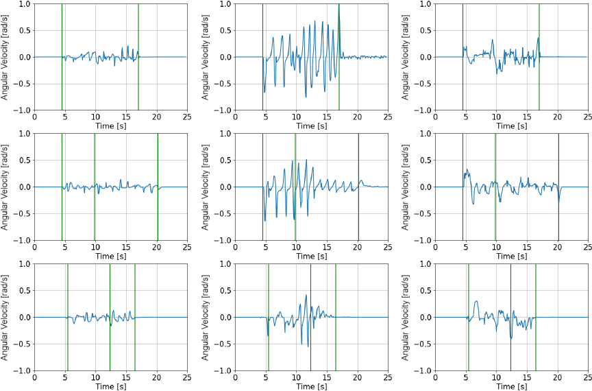
Fig. 5. Example of the measured angular velocity (pitch: left, roll: center, yaw: right) for three obstacle cases: no obstacle (top), obstacle height of 30 mm (middle), and obstacle height of 60 mm (bottom).

2.2. Observational Data and Interpretation

Figures 4 and 5 show the acceleration and angular velocity observed during the experiment, respectively. The sampling interval for the experimental data was \(\mathrm{d}t=0.05\) s. In each figure, the horizontal axis represents the time and the vertical axis represents the acceleration or angular velocity. The two vertical lines at the edges indicate the start and end times of the motor input, whereas the vertical line at the center indicates the collision time (determined visually). In the traveling tests, the robot was able to overcome obstacles up to a height of 40 mm. It overcame obstacles of height of 50 mm in two trials but became stranded in three trials.

These results show that the changes in the measured values around the moment of collision were most prominently reflected in the \(X'\)-axis acceleration. Furthermore, all measured values oscillated at approximately 1–1.5 Hz. This is because the \(X'\)- and \(Z'\)-axes components are affected by gravitational acceleration owing to the pitching motion of the robot (swinging about the \(Y'\)-axis). Based on these findings, the discussion on collision detection focuses on the observed \(X'\)- and \(Z'\)-axes acceleration values.

Furthermore, the accelerations in both the non-stranded case (row 2, column 1 in Fig. 4, obstacle height of 30 mm) and in the stranded case (row 3, column 1 in Fig. 4, obstacle height of 60 mm) show that the pitching motion and measurement noise made it difficult to determine the occurrence of a collision. From these observations, it can be concluded that real-time collision detection based solely on raw sensor data is challenging.

3. Development of Collision Detector

3.1. Mathematical Model of Robot Dynamics Including Unknown Collision Forces

In this section, the robot behavior is modeled as the dynamics of the \(X\)- and \(Z\)-axes accelerations, which include an unknown collision force. The motion of the robot is described in the \(X\)–\(Z\) coordinate system, as follows:

\begin{align} \dot{a}_x(t) &= \alpha_x a_x(t) + \beta_{x0} u_m(t) + \xi\left(t, t_c\right) + \beta_{x2} \omega_x(t),\label{eq:model_ax}\\ \end{align}

\begin{align} \dot{a}_z(t) &= \alpha_z a_z(t) + \beta_{z2} \omega_z(t) + g, \label{eq:model_az}\\ \end{align}

\begin{align} \dot{\theta}(t) &= \alpha_\theta \theta(t) + \beta_{\theta 2} \omega_\theta(t),\label{eq:model_theta} \end{align}

where \(a_x(t)\) is the robot acceleration in the \(X\)-direction, \(u_m(t)\) is the motor power input, and \(\xi(t,t_c)\) is the unknown exogenous input including the collision force and hydrodynamic resistance. \(t_c\) denotes the collision time, \(a_z(t)\) is the robot acceleration in the \(Z\)-direction, and \(\theta(t)\) is the pitch angle. \(\omega_x(t)\), \(\omega_z(t)\), and \(\omega_\theta(t)\) are zero-mean white Gaussian noise sequences with covariance matrices \(\mathrm{cov} \{ \omega_\cdot(t),\, \omega_\cdot(\tau) \} = Q_{\omega\, \cdot} \delta(t - \tau)\). \(g\) is the gravitational acceleration. \(\alpha_x, \alpha_z, \alpha_\theta, \beta_{x0}\), and \(\beta_{x2}\) are assumed to be known and \(\alpha_x, \alpha_z, \alpha_\theta\) are all negative, while \(\beta_{x0}\) and \(\beta_{x2}\) are positive.

In this setting, our goal is to detect collisions by estimating the magnitude of the unknown exogenous input \(\xi(t, t_c)\) and collision time \(t_c\).

To achieve this objective, it is assumed that the unknown collision force is dominant among the exogenous inputs and exhibits a viscous behavior. Accordingly, \(\xi(t, t_c)\) is modeled as follows:

\begin{align} \xi\left(t, t_c\right) = \beta_{x1}v_x(t)u_x\left(t-t_c\right), \end{align}

where \(\beta_{x1}\) is an unknown coefficient representing the magnitude of the collision force, and \(u_x(t-t_c)\) is a step function.

Furthermore, let \(\beta_{x1}\) vary with time to represent the magnitude of the collision force instead of a step function. The collision term is modeled as follows:

\begin{align} \xi\left(t, t_c\right) &= \beta_{x1}\left(t\right)v_x\left(t\right), \label{eq:colterm_ax}\\ \end{align}

\begin{align} \dot{\beta}_{x1}\left(t\right) &= G_{b} \gamma\left(t\right), \label{eq:model_betax1} \end{align}

where \(\gamma(t)\) is a zero-mean white Gaussian noise process with covariance \({\rm cov} \{\gamma(t),\,\gamma(\tau)\} = Q_{\gamma}\delta(t-\tau)\).

Then, by substituting Eq. \(\eqref{eq:colterm_ax}\) into Eq. \(\eqref{eq:model_ax}\), the estimation model is as follows:

\begin{align} \dot{a}_x(t) = \alpha_x a_x(t) + \beta_{x0} u_m(t) + \beta_{x1}(t) v_x(t) + \beta_{x2} \omega_x(t). \label{eq:model_ax_estimate} \end{align}

From Eqs. \(\eqref{eq:model_az}\), \(\eqref{eq:model_theta}\), \(\eqref{eq:model_betax1}\), and \(\eqref{eq:model_ax_estimate}\) and the model of the \(X\)-axis velocity

\begin{align} \dot{v}(t) = a_x(t), \label{eq:model_vx} \end{align}

the state-space representation of the robot dynamics is obtained as follows:

\begin{align} & \begin{bmatrix} \dot{a}_x(t) \\[2pt] \dot{v}_x(t) \\[2pt] \dot{\beta}_{x1}(t) \\[2pt] \dot{a}_z(t) \\[2pt] \dot{\theta}(t) \end{bmatrix} = \begin{bmatrix} \alpha_x & 0 & v_x(t) & 0 & 0 \\ 1 & 0 & 0 & 0 & 0 \\ 0 & 0 & 0 & 0 & 0 \\ 0 & 0 & 0 & \alpha_z & 0 \\ 0 & 0 & 0 & 0 & \alpha_\theta \end{bmatrix} \begin{bmatrix} a_x(t) \\ v_x(t) \\ \beta_{x1}(t) \\ a_z(t) \\ \theta(t) \end{bmatrix} \notag \\ &\quad + \begin{bmatrix} \beta_{x0} & 0 \\ 0 & 0 \\ 0 & 0 \\ 0 & 1 \\ 0 & 0 \end{bmatrix} \begin{bmatrix} u_m(t) \\ g \end{bmatrix} + \begin{bmatrix} \beta_{x2} & 0 & 0 & 0 \\ 0 & 0 & 0 & 0 \\ 0 & G_b & 0 & 0 \\ 0 & 0 & \beta_{z2} & 0 \\ 0 & 0 & 0 & \beta_{\theta 2} \end{bmatrix} \begin{bmatrix} \omega_x(t) \\ \gamma(t) \\ \omega_z(t) \\ \omega_\theta(t) \end{bmatrix}, \end{align}

\begin{align} \dot{z}(t) &= f\left[ t,\, z(t) \right] + B_{u0} \tilde{u}_m(t) + B_{u2} n(t), \label{eq:model_ss_ex_nonlinear} \end{align}

where \(z(t) = [ a_x(t), v_x(t), \beta_{x1}(t), a_z(t), \theta(t) ]^\top\) and \(\mathrm{cov} \{ n(t),\, n(\tau) \} = \mathrm{diag}(Q_{\omega x},\, Q_\gamma,\, Q_{\omega z},\, Q_{\omega\theta} ) \delta(t - \tau) = Q_n(t) \delta(t - \tau)\).

3.2. Observation Equation

The measurements \(y(t)\) were obtained using motion sensors mounted on the robot. The \(X\)- and \(Z\)-axes accelerations were observed as the \(X'\)- and \(Z'\)-axes accelerations oscillated around the \(Y'\)-axis. That is,

\begin{align} y(t) &= \begin{bmatrix} a_x'(t) \\[2pt] a_z'(t) \end{bmatrix} + \omega_v(t) \notag \\ &= \begin{bmatrix} \cos\theta(t) & \sin\theta(t) \\ -\sin\theta(t) & \cos\theta(t) \end{bmatrix} \begin{bmatrix} a_x(t) \\ a_z(t) \end{bmatrix} + \omega_v(t) \notag \\ &= \begin{bmatrix} \cos\theta(t) & 0 & 0 & \sin\theta(t) & 0 \\ -\sin\theta(t) & 0 & 0 & \cos\theta(t) & 0 \end{bmatrix} \begin{bmatrix} a_x(t) \\ v_x(t) \\ \beta_{x1}(t) \\ a_z(t) \\ \theta(t) \end{bmatrix} + \omega_v(t), \end{align}

\begin{align} y(t) &= h\left[ t,\, z(t) \right] + \omega_v(t), \label{eq:model_obs_ex_nonlinear} \end{align}

where \(a_x'(t)\) and \(a_z'(t)\) are the observed accelerations in the \(X'\)–\(Z'\) coordinate system, and \(\omega_v(t)\) is a zero-mean white Gaussian noise process vector with covariance \({\rm cov} \{\omega_v(t),\,\omega_v(\tau)\} = Q_{\omega y}(t)\delta(t-\tau)\).

3.3. Estimation of Unknown Collision Force Using Extended Kalman Filter

The term \(\beta_{x1}(t)\), which represents the magnitude of the unknown collision force, can be estimated using an extended Kalman filter obtained from the linearized Eqs. \(\eqref{eq:model_ss_ex_nonlinear}\) and \(\eqref{eq:model_obs_ex_nonlinear}\).

The linearized form of Eq. \(\eqref{eq:model_ss_ex_nonlinear}\) is as follows (see Appendix A.1 for the procedure):

\begin{align} \dot{z}(t) &= \hat{F}(t) z(t) + u_f(t) + B_{u0} \tilde{u}_m(t) + B_{u2} n(t), \label{eq:model_ss_ex_linear} \end{align}

where

\begin{align} u_f(t) &= f\left[t, \hat{z}\left(t|t\right)\right] - \hat{F}(t) \hat{z}\left(t|t\right), \label{eq:model_ss_ex_linear_uf} \end{align}

and

\begin{align} \hat{F}(t) = \begin{bmatrix} \alpha_x & \hat{\beta}_{x1}(t) & \hat{v}_x(t) & 0 & 0 \\ 1 & 0 & 0 & 0 & 0 \\ 0 & 0 & 0 & 0 & 0 \\ 0 & 0 & 0 & \alpha_z & 0 \\ 0 & 0 & 0 & 0 & \alpha_\theta \end{bmatrix}. \end{align}

Here, \(\hat{z}(t|t)\) is the value in the neighborhood of \(z(t)\). In numerical calculations, the estimated value is used for \(\hat{z}(t|t)\). \(\hat{v}_x(t)\) and \(\hat{\beta}_{x1}(t)\) are the components of \(\hat{z}(t|t)\).

Similarly, the linearization of Eq. \(\eqref{eq:model_obs_ex_nonlinear}\) is obtained as follows (see Appendix A.2 for the procedure):

\begin{align} y(t) &= \hat{H}(t) z(t) + u_h(t) + \omega_v(t),\label{eq:model_obs_ex_linear} \end{align}

where

\begin{align} u_h(t) = h\left[t,\, \hat{z}(t|t)\right] - \hat{H}(t) \hat{z}(t|t), \end{align}

and

\begin{align} \hat{H}(t) &= \left[\begin{array}{cccc} \cos \hat{\theta}(t) & 0 & 0 & \sin \hat{\theta}(t) \\ -\sin \hat{\theta}(t) & 0 & 0 & \cos \hat{\theta}(t) \end{array}\right.\notag\\ & \hspace{2em} \left.\begin{array}{c} \hat{a}_z(t)\cos \hat{\theta}(t) - \hat{a}_x(t)\sin \hat{\theta}(t) \\ \hat{a}_z(t)\sin \hat{\theta}(t) + \hat{a}_x(t)\cos \hat{\theta}(t) \end{array}\right]. \end{align}

\(\hat{a}_x(t)\), \(\hat{a}_z(t)\), and \(\hat{\theta}(t)\) are the components of \(\hat{z}(t|t)\).

Then, assuming that the observations are obtained at discrete time \(\{ t_k \}\) \((k=1,2,\ldots)\), the Kalman filter for Eqs. \(\eqref{eq:model_ss_ex_linear}\) and \(\eqref{eq:model_obs_ex_linear}\) is derived following the procedure described in ¹⁶. The corresponding algorithm is presented in Appendix B.

3.4. Collision Detection via Wavelet Analysis of the Estimated Collision Force

In the previous study ¹³, the estimated magnitude of the collision force \(\hat{\beta}_{x1}(t)\) could be obtained. However, because \(\hat{\beta}_{x1}(t)\) exhibited oscillations similar to those of acceleration, it was difficult to determine the collision time \(t_c\) in real time. Therefore, in this study, a wavelet transform was applied to \(\hat{\beta}_{x1}(t)\) to capture the time-frequency characteristics associated with the collision. The collision time was determined based on these results.

The basic equation of the wavelet transform is as follows:

\begin{align} \left(W_\psi f\right) \left(b,\, a\right) := \left|a\right|^{-\frac{1}{2}}\int_{-\infty}^\infty f(t) \overline{\psi\left(\frac{t-b}{a}\right)}\mathrm{d}t, \end{align}

where \(f(t)\) is the signal to be processed, such as \(\hat{a}_x(t)\) or \(\hat{\beta}_{x1}(t)\). \(\psi(t)\) is the mother wavelet and \(\overline{\psi}(t)\) is the complex conjugate of the mother wavelet. In addition, \(a\) is the scale parameter and \(b\) is the shift parameter.

4. Performance Evaluation with Experimental Data

4.1. Configuration of Collision Detector for Data Analysis

This section presents the results of applying the collision force estimator outlined in Section 3.3 to the acceleration measurements shown in Fig. 4 (with obstacle heights of 0, 30, 40, 50, 55, and 60 mm), as well as the results of applying the wavelet transform to the estimated values presented in Section 3.4.

Table 2 lists the parameters used for the collision force estimator. The motor input \(u_m(t)\) is expressed as follows:

\begin{align} u_m(t) = \left\{\begin{array}{ccl} 0 & {\rm if} & t < t_1,\, t > t_2, \\ 1 & {\rm if} & t_1 \leq t \leq t_2, \end{array}\right. \end{align}

where \(t_1\) is the start time and \(t_2\) is the end time of the motor input. The sampling interval for the observational data was \(\mathrm{d}t=0.05\) s.

Table 2. Parameters and initial conditions for processing experimental data.

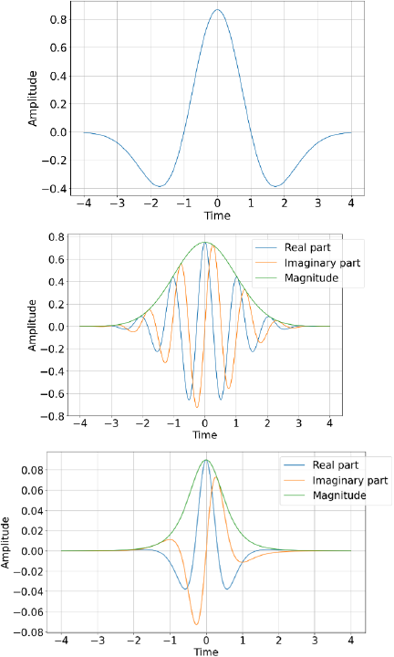
Fig. 6. Shapes of the Mexican Hat (top), Morlet (middle), and Paul (bottom) wavelets.

In the wavelet analysis, the scale parameter \(a\) was set starting from \(s_0=2\times \mathrm{d}t = 0.1\) s with an interval of \(d_j=1/24\) (\(j=1,2,\ldots, 168\)). The shift parameter \(b\) was set to be equal to \(\mathrm{d}t\).

In this analysis, the Mexican Hat, Morlet, and Paul wavelets were used as the mother wavelets. The mother wavelet functions of each wavelet are presented below, and their shapes are shown in Fig. 6.

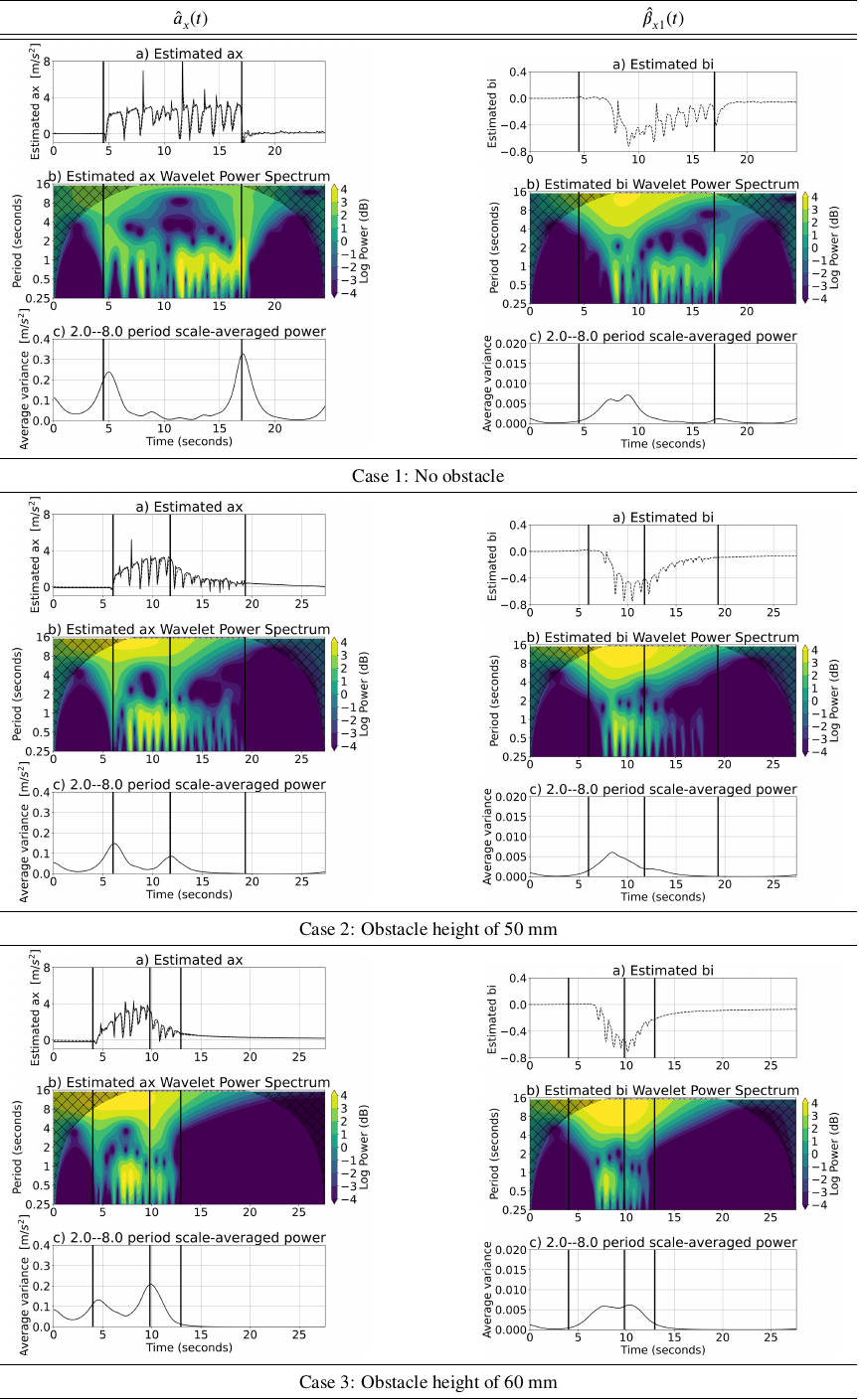
Fig. 7. (a) \(\hat{a}_x(t)\) (left column) and \(\hat{\beta}_{x1}(t)\) (right column), (b) wavelet transforms, and (c) averaged power spectra for obstacle height of 0 mm (Case 1), 50 mm (Case 2; not stranded), and 60 mm (Case 3; stranded).

Mexican Hat wavelet

\begin{align} \psi(t) = \frac{1}{\sqrt{2\pi}} \left( 1 - t^2 \right) e^{-\frac{t^2}{2}} \end{align}

Morlet wavelet

\begin{align} \psi(t) = \pi^{-\frac{1}{4}} e^{i \omega_0 t} e^{-\frac{t^2}{2}}, \end{align}

where \(\omega_0\) is the central angular frequency.

Paul wavelet

\begin{align} \psi_m(t) = \frac{2^m \, i^m \, m!}{\sqrt{\pi (2m)!}} \left( 1 - it \right)^{-(m+1)}, \end{align}

where \(m\) is an integer representing the order of the wavelet that indicates rapidly decaying oscillations. The value of \(m\) is typically taken as \(m \geq 0\), and \(m=4\) was used in this study.

4.2. Results and Discussion

In this study, three types of mother wavelet were applied to the observational data-set. The Paul wavelet was selected because it clearly captures the distinctive features in the wavelet power spectrum around the collision time. The resulting scalogram is shown in Fig. 7.

The figure shows the results for three cases: Case 1: no obstacle, Case 2: an obstacle height of 50 mm without stranding, and Case 3: an obstacle height of 60 mm with stranding. For each case, the left column shows the analysis results for the acceleration \(\hat{a}_x(t)\), while the right column shows the analysis results for the estimated collision force \(\hat{\beta}_{x1}(t)\).

In the left column (acceleration), each figure shows three results. (a) compares the measured \(X'\)-axis acceleration \(a_x(t)\) with the estimated \(X\)-axis acceleration \(\hat{a}_x(t)\), (b) presents the wavelet transform of \(\hat{a}_x(t)\) (the wavelet power spectrum), and (c) shows the wavelet power spectrum averaged over periods of 2–8 s. The details of this averaging are described later. In all figures, the horizontal axis represents the time, whereas the vertical axis represents the magnitude of acceleration in (a), the period of the wavelet power spectrum in (b), and the averaged value of the wavelet power spectrum in (c). In (b), the intensity of the power spectrum is expressed by the color shading.

In the right column (estimated collision force), the difference from the left column is that (a) shows only the time series of the estimated values, while the other figures are structured in the same manner as those in the left column.

As shown in Case 1 (b) in Fig. 7, in the absence of an obstacle, both \(\hat{a}_x(t)\) and \(\hat{\beta}_{x1}(t)\) exhibited prominent components with periods of less than 1 s while the motor was active. In contrast, when an obstacle was present (Cases 2 and 3(b)), these components disappeared after the collision. This suggests that collision detection is feasible using the disappearance of these components as an indicator. However, as the values of \(\hat{a}(t)\) in this range also increased at the start time, reliable collision detection is difficult when relying on them alone.

However, focusing on the 2–8 s period in (b) of \(\hat{a}_x(t)\), no response was observed in Case 1, whereas in the presence of obstacles (Cases 2 and 3), values with a magnitude of approximately 4 dB were observed in the vicinity of the collision time.

To quantify this observation, the wavelet power spectrum in the 2–8 s period shown in (b) was averaged using the following equation:

\begin{align} \overline{W^2\left(s_1, s_2\right)} = \frac{\mathrm{var}\{\delta_j,\, \delta_t\}}{C_\delta} \sum_{j=j_1}^{j_2} \frac{\left| W^2\left(s_j\right) \right|^2}{s_j}, \end{align}

where \(\overline{W^2(s_1, s_2)}\) denotes the averaged wavelet power spectrum over the scale range \(s_1\) to \(s_2\), \(\mathrm{var}\{\delta_j,\, \delta_t\}\) is the variance of the original data, \(\delta_j\) is the scale (frequency) step, \(\delta_t\) is the time step, \(C_\delta\) is the reconstruction coefficient, and \(|W^2(s_j)|\) is the wavelet power at scale \(s_j\). The results are shown in (c) of Fig. 7.

These results indicate that in the case with no obstacles (Case 1), peaks appeared only at the motor start and stop times, whereas in the presence of obstacles (Cases 2 and 3), a peak was also observed at the collision time. That is, because the values in this range increase when the behavior of the robot changes, reliable collision detection becomes difficult when relying solely on them.

To integrate these findings, the trends of the 2–8 s and the 0–1 s components for each robot behavior are summarized in Table 3. The 2–8 s components of \(\hat{a}_x(t)\) showed peaks when the behavior of the robot changed; therefore, it is necessary to distinguish between the effects of the motor inputs and collisions. In contrast, the 0–1 s components of \(\hat{\beta}_{x1}(t)\) changed only at the time of collision. Therefore, the collision time can be determined with high accuracy by jointly evaluating the 2–8 s components of \(\hat{a}_x(t)\) and 0–1 s components of \(\hat{\beta}_{x1}(t)\).

However, because no significant differences were observed in the variation trends of \(\hat{a}_x(t)\) and \(\hat{\beta}_{x1}(t)\) between Cases 2 and 3, it is difficult to determine whether a collision leads to stranding using this method.

Table 3. Trends of components for each robot behavior.

5. Conclusions

In this study, for detecting collisions with soft obstacles using a small paddy-field robot was proposed. In the proposed method, the horizontal and vertical accelerations of the robot are modeled as dynamics including unknown exogenous inputs (e.g., collision forces). The horizontal acceleration and exogenous inputs are estimated using an extended Kalman filter. The exogenous inputs are modeled as viscous terms. Furthermore, wavelet analysis is applied to the estimated values to determine the collision time.

The proposed method was applied to experimental data from a small robot in a paddy field. For the wavelet transform, three types of mother wavelets, namely Mexican Hat, Morlet, and Paul were compared, and the Paul wavelet, which showed the most favorable results, was adopted. The results demonstrated that, for the robot used in this study, collision detection is feasible when using the sub-second components and the 2–8 s components of vibration. By dividing the results of the wavelet transform into several frequency bands, it was shown that the collision time can be determined by evaluating the 2–8 s and 0–1 s components.

Future studies should assess the risk of collisions and determine whether they can lead to stranding.

Appendix A. Linearization of Nonlinear System

The extended Kalman filter is used to construct a Kalman filter when the system or observation equations exhibit nonlinearity ¹⁶. It approximates nonlinear functions by expanding them using a Taylor series or similar methods and treating them as linear for filtering purposes.

A.1. Linearization of Nonlinear System of Robot Dynamics

Consider the nonlinear state-space model:

\begin{align} \dot{z}(t) &= f\left[t, z(t)\right] + B_{u0} \tilde{u}_m(t) + B_{u2}n(t). \tag*{\eqref{eq:model_ss_ex_nonlinear}} \end{align}

Here, assuming that \(f[t, z(t)]\) is a smooth nonlinear function with respect to \(z(t)\), it can be expanded using a Taylor series around the neighborhood of \(\hat{z}(t|t)\) as follows:

\begin{align} f[t,z(t)] &= f\left[t,\hat{z}(t|t)\right] + \hat{F}(t) \left\{ z(t)-\hat{z}\left(t|t\right) \right\} + \cdots, \label{eq:taylor_append} \end{align}

where \(\hat{F}(t)\) is the Jacobian matrix that is expressed as

\begin{align} \hat{F}(t) &= \left.\left[ \frac{\partial f_i(t,z)}{\partial z_i} \right]\right|_{z=\hat{z}(t|t)} = \left.\left[ \frac{\partial }{\partial z}f^\top(t,z) \right]^\top\right|_{z=\hat{z}(t|t)}\nonumber\\[1ex] &= \left.\left[\begin{matrix} \displaystyle\frac{\partial f_1}{\partial z_1} & \cdots & \displaystyle\frac{\partial f_1}{\partial z_n} \cr \vdots & \ddots & \vdots \cr \displaystyle\frac{\partial f_n}{\partial z_1} & \cdots & \displaystyle\frac{\partial f_n}{\partial z_n} \end{matrix}\right]\right|_{z=\hat{z}(t|t)}. \end{align}

\(f_i(t,z)\) and \(z_i\) represent the \(i\)-th elements of the vectors \(f(t, z)\) and \(z\), respectively.

By neglecting the second-order and higher terms in Eqs. \(\eqref{eq:model_ss_ex_nonlinear}\) and \(\eqref{eq:taylor_append}\), the following linear system equation is obtained as an approximation:

\begin{align} \dot{z}(t) &= f\left[t,\hat{z}(t|t)\right] + \hat{F}(t)\left\{ z(t)-\hat{z}(t|t) \right\}\nonumber\\[1ex] &\phantom{=~} + B_{u0} \tilde{u}_m(t) + B_{u2}n(t)\nonumber\\[1ex] &= \hat{F}(t)z(t) + u_f(t) + B_{u0} \tilde{u}_m(t) + B_{u2}n(t),\label{eq:sys_linear_append} \end{align}

where \(u_f(t)=f[t,\hat{z}(t|t)] - \hat{F}(t)\hat{z}(t|t)\).

A.2. Linearization of Nonlinear System of Observation Equation

Consider the nonlinear observation equation:

\begin{align} y(t) &= h\left[ t,\, z(t) \right] + \omega_v(t). \tag*{\eqref{eq:model_obs_ex_nonlinear}} \end{align}

Here, assuming that \(h[t, z(t)]\) is a smooth nonlinear function with respect to \(z(t)\), by applying the same method as the transformation of the state equation, we obtain the following linearized equation:

\begin{align} y(t) &= \hat{H}(t)z(t) + u_h(t) + \omega_v(t), \label{eq:obs_linear_append} \end{align}

where

\begin{align} u_h(t) = h\!\left[t, \hat{z}(t|t)\right] - \hat{H}(t)\hat{z}\left(t|t\right). \end{align}

\(\hat{H}(t)\) is the Jacobian matrix that is expressed as

\begin{align} \hat{H}(t) &= \left.\left[ \frac{\partial h_i(t,z)}{\partial z_i} \right]\right|_{z=\hat{z}(t|t)} = \left.\left[ \frac{\partial}{\partial z} h^\top(t,z) \right]\right|_{z=\hat{z}(t|t)}^\top \notag \\ &= \left.\begin{bmatrix} \dfrac{\partial h_1}{\partial z_1} & \cdots & \dfrac{\partial h_1}{\partial z_n} \\ \vdots & \ddots & \vdots \\ \dfrac{\partial h_m}{\partial z_1} & \cdots & \dfrac{\partial h_m}{\partial z_n} \end{bmatrix}\right|_{z=\hat{z}(t|t)}. \end{align}

Appendix B. Continuous-Discrete Time Kalman Filter

Here, a Kalman filter is considered for the system in which the observed values of the state variable \(z(t)\) at discrete times \(\{t_k\}\) (\(k=1,2,\ldots\)) are obtained through the observation equation for the (linearized) continuous-time system in Eq. \(\eqref{eq:sys_linear_append}\), that is,

\begin{align} \tilde{y}\left(t_k\right) &= \hat{H}\left(t_k\right) z\left(t_k\right) + v\left(t_k\right), \label{eq:obs_append_kalman} \end{align}

where

\begin{align} \tilde{y}\left(t_k\right) := y\left(t_k\right) - u_h\left(t_k\right). \label{eq:obs_yt} \end{align}

Under the assumption that the observed value \(y(t_k)\), predicted value \(\hat{z}(t_k|t_{k-1})\), and \(P(t_k|t_{k-1})\) at time \(t=t_k\) are obtained, the Kalman filter that sequentially obtains the estimates of the state variable \(z(t)\) at observation time \(t=t_k\), that is, \(z(t_k|t_k)\), is expressed as follows:

\begin{align} \hat{z}\left(t_k|t_k\right) &= \hat{z}\left(t_k|t_{k-1}\right) + K\left(t_k\right) \nonumber\\[1ex] & \phantom{==} \cdot \left\{\tilde{y}\left(t_k\right) - \hat{H}(t)\hat{z}\left(t_k|t_{k-1}\right)\right\}, \label{eq:ez_tk}\\[1ex] \end{align}

\begin{align} K(t_k) &= P\left(t_k|t_{k-1}\right) \hat{H}^\top(t_k) \left[\hat{H}(t_k)P\left(t_k|t_{k-1}\right) \right. \nonumber \\[1ex] & \hspace{8.7em} \cdot \left. \hat{H}^\top(t_k)+R(t_k) \right]^{-1}, \label{eq:K_tk}\\[1ex] \end{align}

\begin{align} P\left(t_k|t_k\right) &= P\left(t_k|t_{k-1}\right) - K\left(t_k\right)\hat{H}(t)P\left(t_k|t_{k-1}\right).\label{eq:P_tk} \end{align}

The equation used to obtain the estimate in the interval in which no observations are available, that is, for \(t_k < t < t_{k+1}\), is as follows:

\begin{align} \frac{d\hat{z}\left(t|t_k\right)}{\mathrm{d}t} &= \hat{F}\left(t\right) \hat{z}\left(t|t_k\right), \\[1ex] \end{align}

\begin{align} \left.\hat{z}\left(t|t_k\right)\right|_{t=t_k} &= \hat{z}\left(t_k|t_k\right), \\[1ex] \end{align}

\begin{align} \frac{dP\left(t|t_k\right)}{\mathrm{d}t} &= \hat{F}\left(t\right)P\left(t|t_k\right) + P\left(t|t_k\right) \hat{F}^\top \left(t\right) + B_{u_2} Q_n B_{u_2}^\top,\nonumber \\[1ex] & \\[1ex] \end{align}

\begin{align} \left.P\left(t|t_k\right)\right|_{t=t_k} &= P\left(t_k|t_k\right). \end{align}

Acknowledgments

This study was supported by JSPS KAKENHI Grant Number JP24K07396.

References

[1] M. Seki, H. Nishida, and K. Takahashi, “Development of an environment-harmonized weeding robot system (1st report),” J. of the Japanese Society of Agricultural Machinery, Vol.60, pp. 109-110, 1998 (in Japanese).
[2] M. Seki, H. Nishida, K. Takahashi, and K. Kojima, “Development of an environment-harmonized weeding robot system (2nd report),” J. of the Japanese Society of Agricultural Machinery, Vol.61, pp. 277-278, 1999 (in Japanese).
[3] M. Seki, H. Nishida, K. Takahashi, and K. Kojima, “Development of an environment-harmonized weeding robot system (3rd report),” J. of the Japanese Society of Agricultural Machinery, Vol.62, pp. 51-52, 2000 (in Japanese).
[4] A. Maruyama and K. Naruse, “Development of small weeding robots for rice fields,” 2014 IEEE/SICE Int. Symp. on System Integration (SII 2014), pp. 99-105, 2014. https://doi.org/10.1109/SII.2014.7028019
[5] K. Iwakabe, Y. Yamada, G. Liu, and T. Uejima, “Development of a paddy field mobile robot for the purpose of paddy quality improvement,” Proc. of SICE Annual Conf., pp. 1618-1622, 2013.
[6] K. Iwakabe, S. Kunii, D. Nakai, Y. Yamada, and T. Uejima, “Design and implementation of a paddy field mobile robot for the purpose of paddy quality improvement,” Proc. of 2013 Int. Symp. on Advanced Mechanical Engineering and Power Engineering (ISAMPE2013), 2013.
[7] Y. Iwano, A. Tanaka, and K. Iizuka, “Development of a flail-type mowing system,” J. Robot. Mechatron., Vol.37, No.3, pp. 555-562, 2025. https://doi.org/10.20965/JRM.2025.P0555
[8] S. Haddadin, A. D. Luca, and A. Albu-Schäffer, “Robot collisions: A survey on detection, isolation, and identification,” IEEE Trans. on Robotics, Vol.33, No.6, pp. 1292-1312, 2017. https://doi.org/10.1109/TRO.2017.2723903
[9] Y. Nakagawa and K. Demura, “Collision estimation from information of an omni-directional camera,” The Proc. of JSME Annual Conf. on Robotics and Mechatronics (ROBOMECH2006), Article No.2P1-B04, 2006. https://doi.org/10.1299/jsmermd.2006._2P1-B04_1
[10] M. Hoy, A. S. Matveev, and A. V. Savkin, “Algorithms for collision-free navigation of mobile robots in complex cluttered environments: A survey,” Robotica, Vol.33, No.3, pp. 463-497, 2015. https://doi.org/10.1017/S0263574714000289
[11] M. Yamamoto, Y. Nakashima, M. Hashimoto, and T. Yanaga, “Obstacle-detection bumper for a semi-automatic mower robot suitable for steep slope field,” The Proc. of JSME Annual Conf. on Robotics and Mechatronics (ROBOMECH2018), Article No.2A2-C01, 2018. https://doi.org/10.1299/jsmermd.2018.2a2-c01
[12] H. Nakazawa, K. Nakamura, and K. Naruse, “Collision identification in weeding robot with acceleration sensor,” Proc. of JSPE Conf., pp. 9-10, 2016. https://doi.org/10.11522/PSCJSPE.2016A.0_9
[13] K. Kameyama, D. Mitta, A. Kawasaki, and O. Ankbayar, “Collision detection and stranding prediction of small robots for paddy fields against soft obstacles,” Trans. of the Society of Instrument and Control Engineers, Vol.58, No.4, pp. 213-220, 2022. https://doi.org/10.9746/sicetr.58.213.
[14] K. Kameyama, T. Yasuoka, R. Kawakami, and N. Asai, “G150031 development of the robot to inhibit growth of weeds in the paddy field,” The Proc. of Mechanical Engineering Congress, Japan 2012, pp. G150031-1-G150031-4, 2012. https://doi.org/10.1299/jsmemecj.2012._G150031-1
[15] K. Kameyama and T. Wada, “Adaptation of a small robot for paddy fields to the water depth change using variable legs,” J. Robot. Mechatron., Vol.34, No.1, pp. 159-166, 2022. https://doi.org/10.20965/JRM.2022.P0159
[16] A. Ohsumi, K. Kameyama, and Y. Matuda, “Kalmanfilter and Identification of Systems – An approach to Dynamical Inverse Problem,” Morikita Publishing Co., Ltd., 2016.

This article is published under a Creative Commons Attribution-NoDerivatives 4.0 Internationa License.

[B1] [1] M. Seki, H. Nishida, and K. Takahashi, “Development of an environment-harmonized weeding robot system (1st report),” J. of the Japanese Society of Agricultural Machinery, Vol.60, pp. 109-110, 1998 (in Japanese).

[B2] [2] M. Seki, H. Nishida, K. Takahashi, and K. Kojima, “Development of an environment-harmonized weeding robot system (2nd report),” J. of the Japanese Society of Agricultural Machinery, Vol.61, pp. 277-278, 1999 (in Japanese).

[B3] [3] M. Seki, H. Nishida, K. Takahashi, and K. Kojima, “Development of an environment-harmonized weeding robot system (3rd report),” J. of the Japanese Society of Agricultural Machinery, Vol.62, pp. 51-52, 2000 (in Japanese).

[B4] [4] A. Maruyama and K. Naruse, “Development of small weeding robots for rice fields,” 2014 IEEE/SICE Int. Symp. on System Integration (SII 2014), pp. 99-105, 2014. https://doi.org/10.1109/SII.2014.7028019

[B5] [5] K. Iwakabe, Y. Yamada, G. Liu, and T. Uejima, “Development of a paddy field mobile robot for the purpose of paddy quality improvement,” Proc. of SICE Annual Conf., pp. 1618-1622, 2013.

[B6] [6] K. Iwakabe, S. Kunii, D. Nakai, Y. Yamada, and T. Uejima, “Design and implementation of a paddy field mobile robot for the purpose of paddy quality improvement,” Proc. of 2013 Int. Symp. on Advanced Mechanical Engineering and Power Engineering (ISAMPE2013), 2013.

[B7] [7] Y. Iwano, A. Tanaka, and K. Iizuka, “Development of a flail-type mowing system,” J. Robot. Mechatron., Vol.37, No.3, pp. 555-562, 2025. https://doi.org/10.20965/JRM.2025.P0555

[B8] [8] S. Haddadin, A. D. Luca, and A. Albu-Schäffer, “Robot collisions: A survey on detection, isolation, and identification,” IEEE Trans. on Robotics, Vol.33, No.6, pp. 1292-1312, 2017. https://doi.org/10.1109/TRO.2017.2723903

[B9] [9] Y. Nakagawa and K. Demura, “Collision estimation from information of an omni-directional camera,” The Proc. of JSME Annual Conf. on Robotics and Mechatronics (ROBOMECH2006), Article No.2P1-B04, 2006. https://doi.org/10.1299/jsmermd.2006._2P1-B04_1

[B10] [10] M. Hoy, A. S. Matveev, and A. V. Savkin, “Algorithms for collision-free navigation of mobile robots in complex cluttered environments: A survey,” Robotica, Vol.33, No.3, pp. 463-497, 2015. https://doi.org/10.1017/S0263574714000289

[B11] [11] M. Yamamoto, Y. Nakashima, M. Hashimoto, and T. Yanaga, “Obstacle-detection bumper for a semi-automatic mower robot suitable for steep slope field,” The Proc. of JSME Annual Conf. on Robotics and Mechatronics (ROBOMECH2018), Article No.2A2-C01, 2018. https://doi.org/10.1299/jsmermd.2018.2a2-c01

[B12] [12] H. Nakazawa, K. Nakamura, and K. Naruse, “Collision identification in weeding robot with acceleration sensor,” Proc. of JSPE Conf., pp. 9-10, 2016. https://doi.org/10.11522/PSCJSPE.2016A.0_9

[B13] [13] K. Kameyama, D. Mitta, A. Kawasaki, and O. Ankbayar, “Collision detection and stranding prediction of small robots for paddy fields against soft obstacles,” Trans. of the Society of Instrument and Control Engineers, Vol.58, No.4, pp. 213-220, 2022. https://doi.org/10.9746/sicetr.58.213.

[B14] [14] K. Kameyama, T. Yasuoka, R. Kawakami, and N. Asai, “G150031 development of the robot to inhibit growth of weeds in the paddy field,” The Proc. of Mechanical Engineering Congress, Japan 2012, pp. G150031-1-G150031-4, 2012. https://doi.org/10.1299/jsmemecj.2012._G150031-1

[B15] [15] K. Kameyama and T. Wada, “Adaptation of a small robot for paddy fields to the water depth change using variable legs,” J. Robot. Mechatron., Vol.34, No.1, pp. 159-166, 2022. https://doi.org/10.20965/JRM.2022.P0159

[B16] [16] A. Ohsumi, K. Kameyama, and Y. Matuda, “Kalmanfilter and Identification of Systems – An approach to Dynamical Inverse Problem,” Morikita Publishing Co., Ltd., 2016.