Paper:
Autonomous Agricultural Operations on Slope Terrain by Electric Vehicle Platform
Depeng Chen*
 , Michihisa Iida*
, Masashi Ishii**, and Kazuyoshi Nonami***
, Michihisa Iida*
, Masashi Ishii**, and Kazuyoshi Nonami***
*Graduate School of Agriculture, Kyoto University
Kitashirakawa Oiwake-cho, Sakyo-ku, Kyoto, Kyoto 606-8502, Japan
**Yoka Tekko Co., Ltd.
200 Asakura, Yoka-cho, Yabu, Hyogo 667-0024, Japan
***Faculty of Agriculture, Tottori University
4-101 Koyama-cho Minami, Tottori, Tottori 680-0945, Japan

This study proposes an electric crawler-type robot for autonomous weeding operations on steep slopes. We designed a coverage weeding path for autonomous travel for robots using a global navigation satellite system. The machine was designed to adjust the height of both crawlers to address variations in slope. In addition, the path following the deviation error of the robot with different roll angles was measured. The proposed robot demonstrated optimal performance when the roll angle was set to 17.7°, resulting in an average lateral deviation error of 0.02 m and a weeding area coverage of 99.3%.
Autonomous electric agricultural robot
1. Introduction
Agriculture in the hilly and mountainous regions is an important part of Japanese agricultural production systems. Numerous terraced rice fields “Tanada” remain in these regions; therefore, not only is the flat land cultivated, but mowing the sloping land is also an important agricultural task. These slopes have approximately 40° angles, and the risk of slipping or falling when using manned, self-propelled weed mowers has led to the development of small radio-controlled weed mowers. However, it is difficult to operate radio-controlled mowers on slopes, and there is a demand for autonomous mowers that can be used on slopes.
The gradient of slope environments has a considerable influence on vehicle stability and traction performance, thereby increasing the demand for agricultural machinery 1. The integration of adaptive suspension systems is a pivotal innovation in slope operation. Research has demonstrated that adjustable-height mechanisms can improve the stability by optimizing the center of gravity during an inclined operation 2. This capability is particularly valuable when combined with crawler-type locomotion systems, which provide improved traction and reduced ground pressure compared with wheeled alternatives 3. Yang et al. developed an electric crawler-type weeding robot for a flat onion field that could follow crop rows with high precision 4. Nishimura and Yamaguchi developed a four-wheel grass-cutting robot for steep slopes with an inclination of up to 60°. However, the slippage of the wheel shape used on steep slopes still resulted in unstable movement 5.
In this study, we propose an electric crawler-type weeding robot equipped with a real-time kinematic global navigation satellite system (RTK-GNSS) for weed-mowing operations using autonomous navigation on steep slopes with an inclination of 35°. The contributions of this study can be summarized as follows:
-
(1)
A novel electric vehicle platform featuring adjustable height settings for both left and right crawlers was designed for weed mowing on steep slopes.
-
(2)
An autonomous travelling experiment was conducted based on a target path designed for the required mowing area using GNSS positioning.
-
(3)
The driving performance of the electric weeding robot on slopes at different crawler heights was evaluated using the path-following error and mowing area coverage.
2. Experiment Apparatus
2.1. Overview
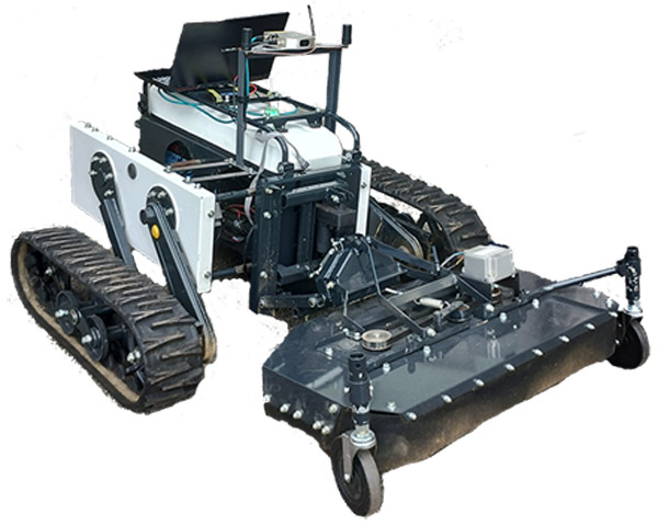
The electric crawler-type weeding robot used in the experiment is shown in Fig. 1. The weed mower was a two-rotor type. The dimensions of the robot were 1650 mm (L) \(\times\) 935 mm (W) \(\times\) 900 mm (H), and its mass was approximately 150 kg. A LiFePO\(_{4}\) battery (DC36 V, 40 Ah) was used as the power source. The robot moved using left and right crawlers driven by independent brushless motors with a gearhead. The weed mower was driven using the same brushless motor without a gear head. These motors had a rated torque of 20 Nm and a rated output of 480 W.
Normally, a farmer can operate a robot in a radio-controlled manner. The robot used an RTK-GNSS (Vision-RTK 2, Fixposition Co., Ltd.) for autonomous operation. When the robot operated in autonomous mode, a notebook PC was used as the host controller. The development environment of the control framework was Robot Operation System (ROS) Noetic. The PC obtained the position and orientation from the RTK-GNSS through Ethernet, processed the data, and sent the control command through the controller area network (CAN).
The robot can mechanically change its tread between 700 mm and 900 mm. Furthermore, the robot can change the height of the left and right crawlers to adjust its attitude toward the sloped terrain.
Fig. 1. The electric crawler-type weeding robot.
2.2. Control Method
The speed control method for the robot involved the transmission of the target speed commands to the left and right motors via the CAN bus, thereby inducing rotation in the crawlers and allowing forward movement of the robot 6. The robot steering method used a two-wheeled vehicle model. The angular velocity \(\omega\) of the vehicle is calculated using Eq. \(\eqref{eq:1}\) as follows:
The speed of the right and left crawler is determined by angular velocity \(\omega\). If the value of \(\omega\) is greater than zero, the vehicle is steering to the left. While if the value of \(\omega\) is less than zero, the vehicle is steering to the right.
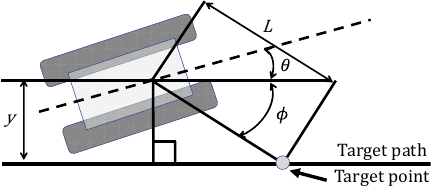
Fig. 2. Lateral and direction deviations from the target.
The angular velocity \(\omega\) is calculated based on the lateral deviation \(y\) and directional deviation \(\theta\) between the vehicle’s current position and target line. As shown in Fig. 2, the target position was located at the end of the straight target line. Distance \(L\) is the distance from the current position to target position. The angle \(\phi\) is the angle from the current position to target point. The target angular velocity \(\omega_{\textrm{d}}\) for the vehicle to turn toward the target position is expressed by Eq. \(\eqref{eq:4}\) as follows:
In this equation, \(\Delta T\) denotes the sampling time of the control process. When angle \(\phi\) is a small value, \(\sin^{-1}(y/L) \simeq {y}/{L}\) can be approximated. Based on the above equations, when given the target speed \(v_{\mathrm{d}}\), speeds of the left crawler \(v_{\mathrm{Ld}}\) and right crawler \(v_{\mathrm{Rd}}\) are calculated with the target angular velocity \(\omega_{\mathrm{d}}\) using Eqs. \(\eqref{eq:5}\) and \(\eqref{eq:6}\) as follows:
The target speeds for the left crawler \(v_{\mathrm{Ld}}\) and right crawler \(v_{\mathrm{Rd}}\) can be calculated, and the referred command value can then be transmitted via the CAN.
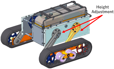
Fig. 3. Roll angle adjustment of the weeding robot.
2.3. Crawler Height Adjustment
As shown in Fig. 3, the heights of the left and right crawlers could be adjusted by changing the fixed angle of the chain case. This chain case was positioned on both the outer sides of the robot’s body and secured in place with screws on each side, allowing for height adjustment. The robot maintained a balanced load distribution by simultaneously changing its rolling angle and chassis width. In the experiment, two crawler heights were selected for autonomous operation on the slopes.
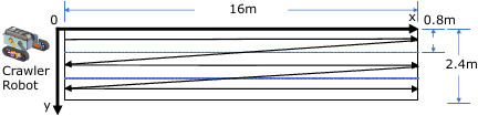
Fig. 4. Experiment routes in experimental area.
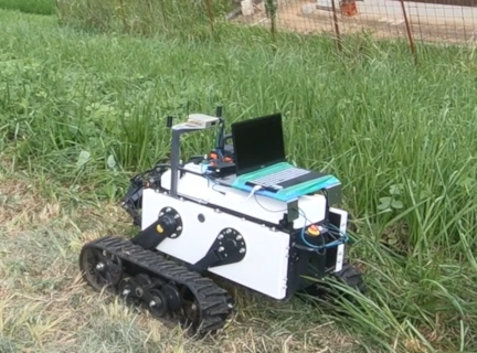
Fig. 5. The weeding robot travelling on slope terrain.
2.4. Route Planning
As shown in Fig. 4, the experimental area was defined by a rectangle. The area was divided into multiple columns for backward and forward operations based on the width of the mower. The rectangular area designated for the experiment was 16 m long and 2.4 m wide. Given the effective width (0.7 m), the area was divided into three lanes. Each lane was assigned start and end points. After reaching the endpoint, the vehicle reverted to the starting point of the adjacent lane and began operation in that new lane.
3. Experiment Method
3.1. Autonomous Navigation Experiment
The field experiment was conducted in a weed area on a steep slope, located in Yabu-cho, Yabu-shi, Hyogo Prefecture, on August 28, 2025 (Fig. 5).
As shown in Fig. 5, the slope of the weed area was 35°. The slope of the experimental area varied only slightly; therefore, the resulting effect was minor. The crawler robot started from the starting point, following the routes described in Section 2.4. Two autonomous navigation experiments were conducted using robots with different roll angles. Owing to mechanical constraints, only roll angles of 10.5° and 17.7° were selected as feasible experimental conditions to represent the optimal outcome achievable within this setup. Other angles were not included in this experiment owing to safety considerations. Experiment 1 was conducted using a robot with a roll angle of 10.5°. Experiment 2 was conducted with a roll angle of 17.7°. In both the experiments, the mowing load was set to the same level. However, this setting was made nonfunctional for safety reasons.
3.2. Evaluation
To evaluate the autonomous travel of the crawler robot, the path-following error and area coverage were evaluated.
3.2.1. Path Following Error
The target path comprised a set of lanes assigned to specific start and end points. For each recorded GNSS point, \(p_{i} = (x_{i}, y_{i})\), the corresponding lane was identified based on the current positions of the start and end points. A continuous working path was formed by sequentially connecting a series of coordinates \((X_{k},Y_{k})\), where \(k\) represents the point index.
For a straight lane, the expected \(y\)-value \(y_{i}^{\mathrm{target}}\) is \(Y_{k}\), which is the \(y\)-value of the starting point (the same as that of the end point). To reverse the backward lane, the expected \(y\)-value \(y_{i}^{\mathrm{target}}\) of the target lane is computed using linear interpolation as follows:
The overall deviation is summarized, including mean error, maximum error, and standard deviation.
3.2.2. Area Coverage
To further evaluate the performance of the weeding operation of the crawler robot, the coverage area of each experiment was evaluated.
The area coverage was determined based on the actual trajectories of the robot and width \(w\). Let the actual GNSS path be represented as a sequence of positions \(P = \sum p_{i}\). Between every pair of adjacent positions, the rectangular area \(R_{i}\) representing weeding coverage was calculated from the distance between two adjacent positions and the mower’s width using the following equation:
Let the area after merging the first \(i\) polygons be denoted as \(A_{\cup}^{(i)}\). When adding the next polygon with area \(R_{i+1}\), the updated union area \(A_{\cup}^{(i+1)}\) is expressed as follows:
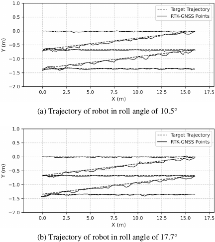
Fig. 6. Autonomous driving trajectories in experimental area.
Table 1. Overall deviation error.

4. Results and Discussion
4.1. Path Following Error
The autonomous driving trajectories in Experiments 1 and 2 using the robot are shown in Fig. 6. The travel trajectory was projected onto a horizontal plane and did not exhibit any changes in elevation. As shown in Fig. 6, the target path is plotted as a dotted line, and the actual travel path recorded by the RTK-GNSS is plotted as a solid line. Both the autonomous driving paths were closely aligned with the target paths. It was demonstrated that the crawler-type electric weeding robot could follow the target path and finish the operation well on the slope area.
Table 1 lists the deviation errors of the two experiments. The average deviations in Experiments 1 and 2 were 0.04 m and 0.02 m, respectively. After the height adjustment of the roll angle for the robot, the deviation error decreased for better performance. The maximum deviation errors were 0.15 m and 0.13 m in two experiments. These errors frequently occur in the reverse path owing to slippage. Experimental observations showed that a roll angle of 17.7° resulted in slightly less slippage than a roll angle of 10.5° during backward motion on a slope. Because of the lack of active control in the roll direction, the observed difference between the tested conditions was marginal.
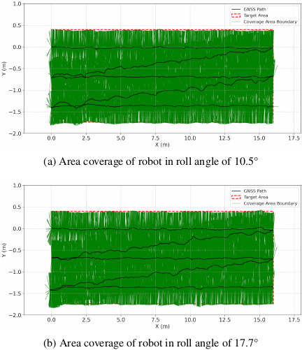
Fig. 7. Area coverage illustration of experiments.
Table 2. Overall area coverage.

4.2. Area Coverage Results
Figure 7 shows the area coverage of the weeding performance during autonomous driving following the target path. The black lines represent the actual travel paths of the mowing-robot-recorded GNSS positioning system. Green lines indicate the length of the mower’s width and recorded position.
The overall coverage areas are listed in Table 2. The target coverage areas in both experiments were 34.24 m\(^2\). The actual coverage areas in Experiments 1 and 2 were 33.96 m\(^2\) and 34.0 m\(^2\), respectively. Both coverage percentages were greater than 99%. The weeding performance of the electric vehicle was acceptable in the sloped area.
5. Conclusions
This study proposes a novel electric vehicle platform for weed mowing on steep slopes. An autonomous travel experiment was conducted to assess the path-following error and weeding coverage area with various adjustable height settings for both the left and right crawlers. The key conclusions are summarized as follows:
-
(1)
Autonomous travel experiments were successfully conducted by following a designed path for the required mowing area, using GNSS positioning.
-
(2)
The path-following errors of the electric weeding robot on a slope with an inclination of 35° at different crawler heights were evaluated. The average lateral deviation errors were 0.04 m and 0.02 m for the robot at roll angles of 10.5° and 17.7°, respectively. The path-following accuracy was high for autonomous agricultural operations on steep slopes.
-
(3)
The required mowing areas in both experiments were 34.24 m\(^2\). The actual coverage area was 33.96 m\(^2\) and 34.0 m\(^2\) for the robot at roll angles of 10.5° and 17.7°, respectively.
The experimental results indicate that the proposed robot can accomplish autonomous travel on steep slopes using GNSS positioning. Future study will focus on developing an improved target path to lower the lap rate and operation time, save energy, and increase the efficiency of operations.
Acknowledgments
This study was supported by the Development and Supply Program of Smart Agricultural Technology Grant (JPJ013136) from the Project of the Bio-Oriented Technology Research Advancement Institution (BRAIN).
- [1] F. Yang et al., “Development and validation of sloped ground pressure prediction model for a tracked tractor in hilly and mountainous environments,” Soil Tillage Res., Vol.241, Article No.106135, 2024. https://doi.org/10.1016/j.still.2024.106135
- [2] H.-P. Liu, F.-Z. Yang, S. Liu, and Y. Lu, “Effect of mechanism of height difference on stability of miniature crawler hillside tractor,” Tract. Farm Transp., Vol.40, No.1, pp. 18-21, 2013 (in Chinese).
- [3] R. Vidoni, M. Bietresato, A. Gasparetto, and F. Mazzetto, “Evaluation and stability comparison of different vehicle configurations for robotic agricultural operations on side-slopes,” Biosyst. Eng., Vol.129, pp. 197-211, 2015. https://doi.org/10.1016/j.biosystemseng.2014.10.003
- [4] L. Yang, S. Kamata, Y. Hoshino, Y. Liu, and C. Tomioka, “Development of EV crawler-type weeding robot for organic onion,” Agriculture, Vol.15, No.1, Article No.2, 2025. https://doi.org/10.3390/agriculture15010002
- [5] Y. Nishimura and T. Yamaguchi, “Grass cutting robot for inclined surfaces in hilly and mountainous areas,” Sensors, Vol.23, No.1, Article No.528, 2023. https://doi.org/10.3390/s23010528
- [6] H.-Y. Hsu et al., “Automatic mowing by an electric agricultural machine,” J. Jpn. Soc. Agric. Mach. Food Eng., Vol.86, No.6, pp. 420-428, 2024 (in Japanese). https://doi.org/10.11357/jsamfe.86.6_420
This article is published under a Creative Commons Attribution-NoDerivatives 4.0 Internationa License.