Paper:
Comparative Analysis of PALSAR-2 and Geographical Features for Mapping Urban and Non-Urban Flooded Areas
Ryosuke Nagato*, Ira Karrel San Jose*
 , Sesa Wiguna**
, Ryohei Kametaka*
, Bruno Adriano**
, Erick Mas**
, and Shunichi Koshimura**,†
, Sesa Wiguna**
, Ryohei Kametaka*
, Bruno Adriano**
, Erick Mas**
, and Shunichi Koshimura**,†
*Department of Civil and Environmental Engineering, Tohoku University
6-6-06 Aramaki Aza-Aoba, Aoba-ku, Sendai, Miyagi 980-8579, Japan
**International Research Institute of Disaster Science, Tohoku University
Sendai, Japan
†Corresponding author

Owing to recent extreme weather events, flood risk has been rising annually, increasing the demand for fast and accurate flood mapping. Synthetic aperture radar imagery has received considerable attention for flood-mapping applications owing to its all-weather, day-and-night imaging capabilities. Although previous studies have achieved accurate mapping in non-urban areas, challenges remain for urban regions. This study focuses on flood events in Japan by employing a deep learning model and PALSAR-2 imagery to classify non-flooded areas, floods in open areas, and floods in urban areas. To understand the complex spectral characteristics specific to urban areas, this study investigates the integration of geographical features, such as slope and building footprints, into the segmentation process. The experimental results suggest that the inclusion of these supplementary data improves the prediction performance of the trained models.
Flood mapping using SAR and geographical features
1. Introduction
Flooding is one of the most destructive natural hazards worldwide, affecting billions of people and having severe social, economic, and environmental impacts 1,2. The consequences of floods are projected to worsen under changing climate conditions, as irregular weather patterns and intensified rainfall events have increased the frequency and severity of inundation in many regions 3. Under such circumstances, timely and accurate flood mapping becomes vital not only to support immediate disaster response but also to inform long-term risk reduction and resilience strategies. Remote sensing data, such as satellite imagery and aerial photographs, serve as effective tools for rapidly assessing damage over vast areas 4. They are widely used to efficiently identify inundated areas, particularly in situations where on-site surveys are not feasible. Compared with physics-based hydrodynamic models and other numerical inundation mapping techniques, the interpretation of remote sensing data often requires relatively fewer input data, facilitating faster flood detection and analysis. However, cloud cover associated with rainfall during floods often hinders the use of optical satellites and aerial imagery.
To address these limitations, synthetic aperture radar (SAR) has been widely used in flood-related studies. Unlike optical sensors, SAR can penetrate clouds and acquire observations under day and night conditions, making it well-suited for investigating hydrological disasters. Multiple studies have demonstrated the effectiveness of SAR-based flood mapping, particularly in open landscapes such as croplands, wetlands, and bare soil, where water bodies typically exhibit a strong contrast against the surrounding land cover 5,6,7,8,9.
Despite these advances, urban flood detection remains a challenge. Built-up environments introduce complex SAR backscattering effects owing to the contrast in surface reflectance produced by buildings, roads, and other heterogeneous surfaces. These conditions lead to phenomena such as layover, shadowing, and double-bounce reflections, which complicate the separation of inundated and non-inundated surfaces 10. Consequently, although SAR-based approaches have demonstrated strong performance in rural and open settings, their accuracy in dense urban areas remains limited 11. This limitation is particularly concerning, as urban regions concentrate populations, critical infrastructure, and economic activities, thereby amplifying the consequences of flood hazards.
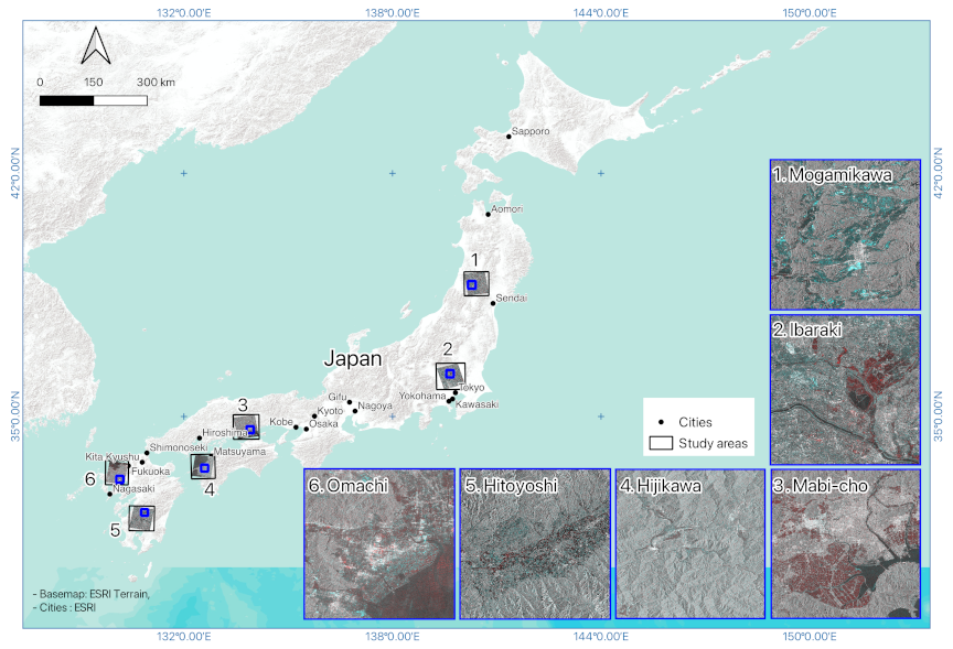
Fig. 1. Study area. Images 1–6 depict RGB composites of the six flood sites evaluated. The red channel corresponds to pre-event SAR imagery, whereas the green and blue channels represent post-event SAR imagery.
To improve flood detection in built-up zones, recent studies have begun to integrate SAR with auxiliary geospatial datasets 12. For instance, Tavus et al. 13 demonstrated that combining pre- and post-event Sentinel-1 imagery with DEM-derived topographic information enhanced flood segmentation in mixed land cover settings. Similarly, Baghermanesh et al. 14 demonstrated the potential of fusing TerraSAR-X with LiDAR-based surface models to reconstruct scattering mechanisms, such as double-bounce and layover, thus sharpening the detection of floods in dense city centers. These studies highlight the importance of topographic and structural information for interpreting SAR backscatter more effectively.
In this context, this study employs high-resolution L-band SAR images (ALOS-2 PALSAR-2, 3 m), slope information derived from a digital elevation model (DEM), and building footprint data. Compared with the widely used C-band Sentinel-1 imagery, L-band SAR, which partially penetrates vegetation and small structures and suppresses unnecessary scattering, may facilitate the learning of subtle flood characteristics in urban areas. The influence of slope and building information is systematically assessed to quantify the added value of the auxiliary datasets for enhancing SAR-based flood detection in both urban and open areas.
2. Dataset
This study employs multi-source datasets that integrate SAR imagery and geographical features. Specifically, ALOS-2 PALSAR-2 images, DEM-derived slope data, and building footprint information were used to examine six major flood events in Japan, as illustrated in Fig. 1. The events were selected based on two criteria: (1) all events that occurred within the past ten years; and (2) the availabiluty of ground-truth flood extent maps, PALSAR-2 images, DEMs, and building information for the affected sites.
Additionally, the SAR image presented in Fig. 1 is an RGB image created using the SAR intensity and coherence values from the pre- and post-event phases.
Table 1. Details of the evaluated flood events.

Table 2. Event dates, acquisition dates, and sources of ground-truth data for each flood event.

2.1. ALOS-2 PALSAR-2 Imagery
Multi-temporal ALOS-2 PALSAR-2 data provided by the Japan Aerospace Exploration Agency (JAXA) were used in this study. For each flood event, images from both pre- and post-event periods were obtained, with acquisition dates listed in Table 1. The flood areas correspond to the areas in each ground-truth data polygon. The images were collected in the Stripmap Ultrafine mode, which provides a satisfactory spatial resolution of 3 m, and were recorded in HH polarization.
SAR backscatter intensity images were generated for each acquisition period to capture surface scattering characteristics before and after flooding. In addition, SAR coherence was computed from paired pre- and post-event images, which indicates the similarity of backscatter signals over time. Coherence is particularly useful for flood mapping, as areas affected by inundation typically exhibit a significant reduction in coherence compared with non-flooded regions. All SAR data processing, including radiometric calibration, geocoding, and coherence generation, was conducted using the ENVI software. During the preprocessing stage, a \(1\times1\) multi-look filter was applied, and a Lee filter with a \(3\times3\) window size was used for speckle reduction. SRTM3 version 4 was used for geocoding.
2.2. DEM-Derived Slope Data
Topographic information was incorporated using DEM data obtained from the Geospatial Information Authority of Japan (GSI). The original DEM, with a spatial resolution of 5 m, was resampled to 3 m to match the resolution of the SAR imagery. Rather than using elevation, which provides limited information on flood susceptibility, slope was derived from the DEM and used as the primary topographic feature in this study.
Slope, expressed in degrees, was calculated as
2.3. Building Footprints
Information on built-up areas was extracted from the building footprints obtained from the GSI. Initially, these were provided in a vector format and rasterized to align with the spatial resolution of the SAR images. The rasterized footprints were binarized, where a pixel value of 1 corresponded to building structures and a value of 0 represented non-building areas.
This geographical feature is key for flood mapping in urban settings, where the presence of buildings significantly affects SAR backscatter. The inclusion of building data may help identify flooded urban areas.
2.4. Ground-Truth Data
Reference data for model training and evaluation were derived from the flood extent polygons provided by the GSI and Liu and Yamazaki 15. The land cover map was produced by JAXA. The acquisition dates and data providers for the flood extent polygons are listed in Table 2.
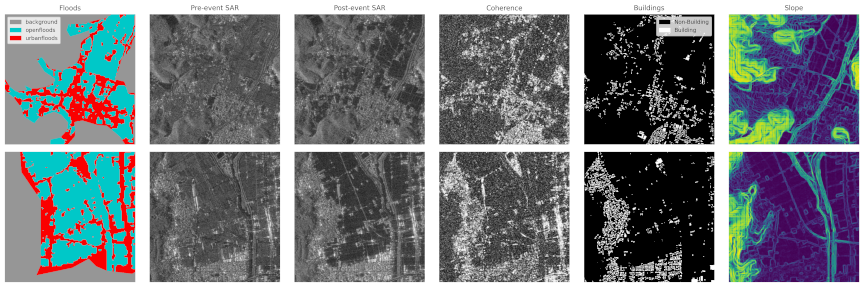
Fig. 2. Samples of the dataset used (from left to right: flood mask, pre-event SAR images, post-event SAR images, coherence, building footprint, and slope).
By overlaying the two datasets, three classes were established: (1) flooded urban areas (FUA), denoting regions where flood extent polygons overlap with urban land cover; (2) flooded open areas (FOA), representing inundated zones outside urban regions; and (3) non-flooded areas (NF), depicting unaffected terrain. The generated flood masks were rasterized to the exact spatial resolution of the SAR images to ensure compatibility during model training and testing. Fig. 2 depicts examples of ground-truth data.
3. Methods
This section describes the experimental methods, including the deep learning model, training settings, evaluation metrics, and input mode scenarios.
3.1. Deep Learning
In this study, flood extent detection is treated as a semantic segmentation task, where each pixel in the input imagery is classified into predefined categories (e.g., flooded or non-flooded). The U-Net architecture 21 was used for a semantic segmentation task. The U-Net was initially developed for biomedical image segmentation and has been widely applied across diverse disciplines owing to its ability to learn spatial representations from input data. The encoder-decoder design captures both contextual and fine-grained spatial information. Simultaneously, the skip connections between the encoder and decoder layers preserve information during downsampling by reintroducing spatial features at the decoding stage.
The U-Net model was implemented using the Segmentation Models PyTorch with EfficientNet-B4 22 backbone and scSE attention module 23. The final layer of the model was modified to accommodate the number of classes defined in the study. The number of input channels varied depending on the number of layers fed into the network. Pretrained weights from ImageNet were used for initialization, and the model was then trained using the input datasets 24.
3.2. Training Settings
All input images were resized to \(512 \times 512\) pixels before training. The model was trained for 120 epochs with a batch size of 16. Optimization was performed using the Adam optimizer with an initial learning rate of \(1 \times 10^{-4}\). To address class imbalance and improve the segmentation accuracy for minority classes, Dice loss was adopted as the cost function, as it directly optimizes the overlap between predicted and ground-truth masks 25,26. To evaluate the robustness of the model, training was repeated with three different random seeds (100, 200, and 300). This allowed for the assessment of the model’s performance and consistency across different initializations. A summary of the training parameters is provided in Table 3. Each SAR image was divided into samples with a resolution of 3 m and a size of \(512\times512\) pixels. A total of 1,032 samples were used for training, and 282 samples were used for testing and evaluation.
Table 3. Training parameters.

3.3. Evaluation Metrics
The performance of the model was evaluated using three commonly adopted metrics for binary classification: precision, recall, and F1-score. These metrics are computed at the pixel level to assess the segmentation quality.
Precision refers to the proportion of predicted flooded pixels, as expressed in Eq. \(\eqref{eq:precision}\):
Recall evaluates the model’s ability to capture all actual flooded pixels. This is defined in Eq. \(\eqref{eq:precision}\):
F1-score provides a balanced measure that combines precision and recall into a single metric. This is defined as the harmonic mean of the two:
The F1-score ranges between 0 and 1, with values closer to 1 indicating that the model achieves both high precision and high recall. In the context of flood detection, a high F1-score implies that the model is effective not only in minimizing false alarms but also in reducing missed detections. Additionally, as the F1-score considers precision and recall, it is suitable for measuring scores in imbalanced samples.
Table 4. Input mode scenarios.

3.4. Input Mode Scenarios
In this study, the effectiveness of integrating geographical features to detect urban and open areas was examined by evaluating the performance of a model using different input modes as shown in Table 4. The first mode, Mode 1, uses only the post-event SAR image as the input, serving as the baseline mode. In Mode 2, additional data in the form of a slope were incorporated along with post-event SAR images. Mode 3 introduced building footprint data in combination with post-event SAR images.
The next set of modes focuses on multi-temporal data and geospatial features. In Mode 4, the pre-event SAR image was added to the post-event SAR image to capture temporal changes. Mode 5 further extended this configuration by including the slope in addition to the pre-event and post-event SAR images. Mode 6 introduced building footprint data along with pre- and post-event SAR images, enabling a more comprehensive understanding of temporal and spatial dynamics.
Mode 7 combined both the pre-event and post-event SAR image with the coherence image generated from these two SAR images. This mode aimed to leverage the coherence between the two datasets to improve the flood detection process.
Finally, in Mode 8, all available features were integrated, including the post-event SAR image, pre-event SAR image, coherence, slope, and building footprint. This full modality aimed to provide the most comprehensive input data for the model, combining both temporal and geospatial features to optimize flood detection performance. Each mode was designed to progressively add more input data, allowing the evaluation of the impact of these features on model performance.
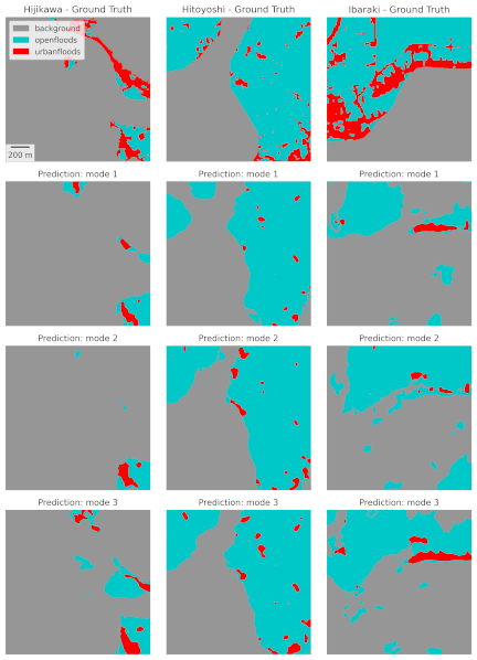
Fig. 3. Sample flood prediction results based on post-event SAR imagery, slope, and building footprints. The top row illustrates the ground truth for the three flood events (gray: NF, blue: FOA, and red: FUA).
4. Results and Discussion
4.1. Post-Event and Geographical Features
The first three experiments focused on unitemporal input settings to evaluate the extent to which supplementary geospatial features could compensate for the absence of temporal information. An example of the results is shown in Fig. 3. In Mode 1, which used only post-event SAR imagery, the model achieved relatively high performance in identifying NF regions. However, its performance significantly decreased in detecting flooded areas, particularly in urban settings, where the F1-score was only 0.404.
Mode 2 incorporated slope data alongside post-event SAR. Modest improvements were observed across all categories. Specifically, in FUA, the F1-score increased to 0.437, indicating that slope data may help recognize topographic patterns associated with flooding. However, this advantage remains limited to complex urban areas, where man-made structures have a greater influence on radar backscatter than elevation.
In Mode 3, which used building footprint data instead of slope data, the FUA score increased further to 0.443, slightly surpassing that of Mode 2. This increase suggests that building information offers a more effective contextual cue for identifying flooded urban areas, even without temporal data. Although the improvement was small, this finding indicates that building footprints, although static, offer more useful spatial cues than slopes when classifying FUA pixels under single-date conditions.
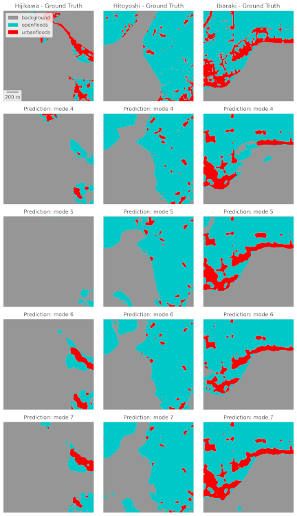
Fig. 4. Sample flood prediction results based on multi-temporal SAR imagery (pre- and post-event), slope, building footprints, and coherence. The top row illustrates the ground truth for the three flood events (gray: NF, blue: FOA, and red: FUA).
4.2. Multi-Temporal and Geographical Features
This subsection presents the results of the configurations that include both pre- and post-event SAR images, allowing the model to capture temporal changes associated with inundation. An example of the results is shown in Fig. 4. The improvement in the FUA score from 0.404 in Mode 1 (post-event SAR imagery) to 0.481 in Mode 4 (pre- and post-event SAR imagery) emphasizes the importance of temporal information, particularly in urban areas where SAR backscatter is often complex.
When slope information was introduced alongside pre- and post-event SAR imagery in Mode 5, the FUA score slightly decreased compared with that in Mode 4. This suggests that, although the slope provided additional contextual information when using only post-event SAR data, its contribution diminished when temporal change detection was applied. Moreover, this finding is consistent with that of 27, where the inclusion of topographical information derived from DEM had limited effects on flood detection using multi-temporal SAR data, particularly in flat terrains. Nevertheless, slope appears to play a supportive role primarily when a multi-temporal analysis is unavailable.
In contrast, the inclusion of building footprints (Mode 6) or coherence (Mode 7) led to a better performance in the FUA class, with both modes slightly exceeding the score of Mode 4, which used only multi-temporal SAR data. Building footprints provide the location and distribution of structures that guide the model in localizing flooded urban areas. However, coherence highlights the changes in surface reflectance, which further improves flood detection accuracy as also indicated by the works of 28 and 29. Both modes achieved the highest FUA F1-scores within this group (0.492 and 0.483), suggesting that building footprints and coherence complement multi-temporal SAR information in identifying inundated zones.
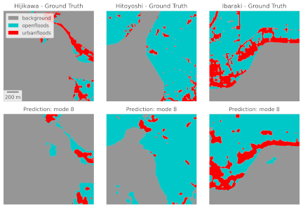
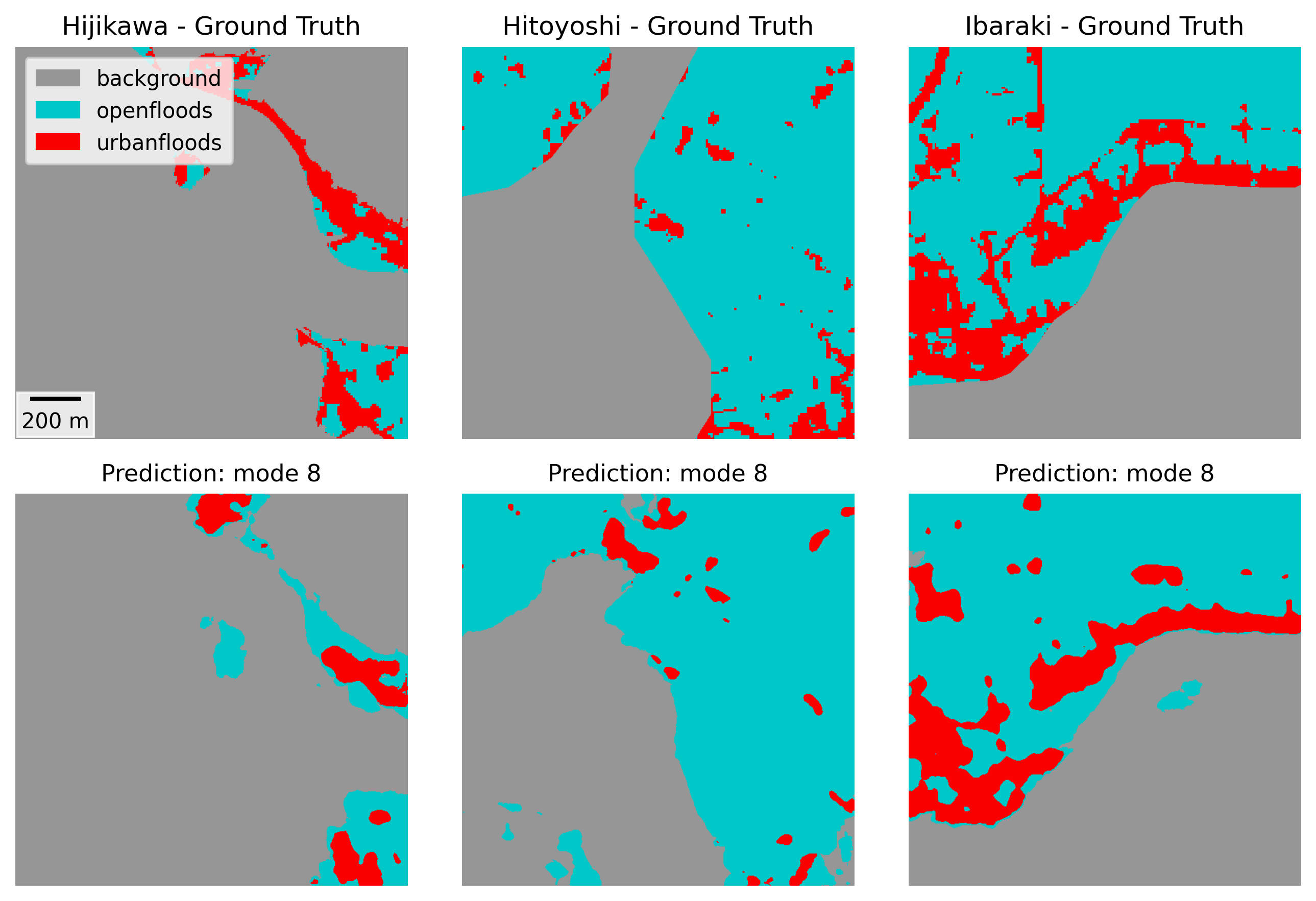
Fig. 5. Sample flood prediction results based on the integration of all datasets (multi-temporal SAR imagery, slope, building footprints, and coherence). The top row illustrates the ground truth for the three flood events (gray: NF, blue: FOA, and red: FUA).
In general, the flood detection improved with the inclusion of pre-event SAR imagery in the model. Furthermore, additional information extracted from building footprints and coherence contributed to improved detection in urban areas.
Table 5. Summary of model performance based on F1-scores of NF, FOA, and FUA.

4.3. Full Modality
In Mode 8, all available inputs, including pre- and post-event SAR imagery, slope, building footprints, and coherence, were integrated. This configuration provided the best overall results. An example of the results is shown in Fig. 5. However, the performance margin between Mode 8 and Modes 6 and 7 was relatively small, with a mean score of approximately 0.004. While integrating all the input data into the model delivered the highest accuracy, the slight improvement in distinguishing flooded areas in both urban and open regions may not justify the additional data requirements and processing, particularly in real-time or large-scale applications. Nevertheless, this outcome demonstrates the advantage of combining temporal change information with additional geographic features, resulting in a slightly more robust model across NF, FOA, and FUA.
4.4. Comparison of Selected Best Modes
Table 5 lists the modes with the highest score within post-event features, multi-temporal features, and full modality. The unitemporal modes (Modes 1–3) establish the baseline for urban floods. Using only post-event SAR (Mode 1) results in a low FUA of 0.404, despite a strong NF. Adding slope (Mode 2) nudges FUA to 0.437, and adding buildings (Mode 3) further increases it to 0.443. Under only post-event SAR data conditions, both geographic features help FUA, with buildings providing the larger changes in FUA.
Introducing temporal information is a primary step forward. With pre- and post-event SAR (Mode 4), the FUA increases to 0.481. In this multi-temporal approach, the effects of added features diverge for FUA: slope (Mode 5) lowers it to 0.465, buildings (Mode 6) increase it to 0.492, and coherence (Mode 7) yields a slight increase to 0.483. This pattern suggests that temporal SAR differences largely absorb terrain features, whereas urban structures (such as buildings) remain discriminative, and coherence stabilizes change cues. Moreover, FOA benefits substantially from moving to multi-temporal inputs (from \(\approx0.71\) in Mode 3 to \(\approx0.77\) in Modes 4–7), and NF increases up to 0.917.
The full modality, Mode 8, presents the best overall balance with the top urban score \(\mathrm{FUA} = 0.50\), \(\mathrm{FOA} \approx 0.77\), and \(\mathrm{NF} \approx 0.92\). However, the increments are small (\(\pm 0.017\) between Modes 7 and 8 and \(\pm 0.008\) between Modes 6 and 8) for FUA, and FOA/NF move minimally from the multi-temporal baselines. As Mode 8 adds buildings and slopes simultaneously, we cannot attribute the gain to a single feature. The most consistent interpretation is that buildings and coherence underpin urban improvement. In contrast, slope contributes minimally when temporal information is present. Therefore, the best input mode in this study was Mode 8.
However, from an efficiency perspective, the pre/post-SAR, buildings, and coherence combination stands out as the most impactful configuration for urban floods, as they focus on the most important features for FUA while keeping the input complexity low. Although Mode 8 remains the best overall, its small edge over Modes 7 and 6 indicates that carefully refined combinations could approach, possibly even match, Mode 8 for FUA without significantly impacting FOA/NF.
5. Conclusion
This study aimed to quantify how geographic features (slope and building footprints) contribute to improving SAR-based flood mapping by prioritizing FUA, followed by FOA and NF. We evaluated the class-wise F1-scores among the eight input modes.
Under unitemporal inputs, both geographic features added value to FUA, but buildings contributed more than slope: beginning from post-event SAR alone (FUA = 0.404), adding slope raised FUA to 0.437 (+0.033), while adding buildings increased it to 0.443 (+0.039). The effects on FOA and NF were modest.
The primary step forward was temporal information. With pre- and post-SAR (Mode 4), the FUA increased to 0.481. On this multi-temporal base, the marginal contribution of each feature could be quantified for FUA: the slope lowered FUA to 0.465 (\(-0.016\)), buildings increased it to 0.492 (\(+0.011\)), and coherence slightly increased it to 0.483 (+0.002). Thus, terrain features were largely subsumed once temporal differences became available, whereas urban structures remained informative and stabilized surface changes in coherence. For the FOA, the increments were primarily due to temporal information and coherence; NF rapidly saturated at 0.917.
The full modality (Mode 8) combined all the inputs and achieved the best overall performance. The increment over Mode 7 was small, and minor variations in FOA and NF indicated that most of the urban gain had already been realized by pairing temporal SAR with building information and coherence. As buildings and slopes enter simultaneously in Mode 8, we do not ascribe the final gain to a single feature; taken together with the ablations, the quantitative pattern is consistent with buildings (\(+0.011\) on the multi-temporal base) and coherence (\(+0.002\)), underpinning FUA improvements. In contrast, the slope adds a limited value and can be detrimental to the FUA (\(-0.016\)) once temporal information is present.
Despite the overall improvements, the FUA class remains the most challenging. Two interacting factors explain why gains in urban areas tend to saturate. First, the urban-specific scattering geometry fundamentally disrupts the simple “water gets darker” rule. High-rise and mid-rise blocks create layover and radar shadows that suppress backscatter, irrespective of whether the ground is flooded, yielding systematic false negatives. Conversely, double-bounce between vertical walls and horizontal surfaces (streets, courtyards) often remains bright and can even brighten when a thin water film is present; therefore, flooded and dry states can be radiometrically indistinguishable. At 3 m resolution, narrow streets and building canyons span only a few pixels, leading to sub-pixel mixing of walls, asphalt, vegetation, and water, which further blurs the class boundaries. Second, the building footprints we used are purely planimetric (2D) and carry no information about height or facade orientation, the variables that govern where layover, shadow, and double-bounce occur. Without 3D context, the network cannot reliably distinguish between bright returns caused by dry ground double-bounce and those caused by wall water interactions, nor can it anticipate shadowed zones where intensity is low, irrespective of inundation. Consequently, adding 2D footprints improves the localization of built-up areas, but does not resolve the core ambiguity imposed by urban scattering physics.
In summary, multi-temporal SAR acts as a foundation, whereas geographic features add extra value when integrated selectively.
This study focuses on isolating the contributions of individual geospatial features. Therefore, a future direction would be to investigate the best combinations of selected features, such as pre- and post-event SAR imagery, building data, and coherence, while excluding less impactful features such as slope. Such configurations could potentially outperform Mode 8, particularly in detecting FUA, and provide a more efficient balance between performance and data complexity.
In addition, although it is an approach applied to wetlands rather than floods, we would like to consider methods such as those proposed by McCormack et al. 30, which improve accuracy by removing pixels that are prone to SAR misclassifications or have a low likelihood of inundation.
Acknowledgments
This study was supported by JSPS KAKENHI (21H05001), the Project Grant from the Co-creation Center for Disaster Resilience, IRIDeS, Tohoku University (ID:1-DT020), the JAXA EO-RA4 Project (ID: ER4A2N09), JST SICORP (JPMJSC2311), and the SIP Program of CSTI (JPJ012289).
- [1] J. Rentschler, M. Salhab, and B. A. Jafino, “Flood exposure and poverty in 188 countries,” Nature Communications, Vol.13, No.1, Article No.3527, 2022. https://doi.org/10.1038/s41467-022-30727-4
- [2] Centre for Research on the Epidemiology of Disasters (CRED) “The human cost of weather-related disasters 1995–2016,” United Nations Office for Disaster Risk Reduction (UNDRR), Technical report, 2015.
- [3] S. A. Kulp and B. H. Strauss, “New elevation data triple estimates of global vulnerability to sea-level rise and coastal flooding,” Nature Communications, Vol.10, Article No.4844, 2019. https://doi.org/10.1038/s41467-019-12808-z
- [4] P. C. Oddo and J. D. Bolten, “The value of near real-time earth observations for improved flood disaster response,” Frontiers in Environmental Science, Vol.7, Article No.127, 2019. https://doi.org/10.3389/fenvs.2019.00127
- [5] B. Bauer-Marschallinger, S. Cao, M. E. Tupas, F. Roth, C. Navacchi, T. Melzer, V. Freeman, and W. Wagner, “Satellite-based flood mapping through Bayesian inference from a Sentinel-1 SAR datacube,” Remote Sensing, Vol.14, No.15, Article No.3673, 2022. https://doi.org/10.3390/rs14153673
- [6] X. Jiang, S. Liang, X. He et al., “Rapid and large-scale mapping of flood inundation via integrating spaceborne synthetic aperture radar imagery with unsupervised deep learning,” ISPRS J. of Photogrammetry and Remote Sensing, Vol.178, pp. 36-50, 2021. https://doi.org/10.1016/j.isprsjprs.2021.05.019
- [7] J. Li, L. Li, Y. Song, J. Chen, Z. Wang, Y. Bao, W. Zhang, and L. Meng, “A robust large-scale surface water mapping framework with high spatiotemporal resolution based on the fusion of multi-source remote sensing data,” Int. J. of Applied Earth Observation and Geoinformation, Vol.118, Article No.103288, 2023. https://doi.org/10.1016/j.jag.2023.103288
- [8] Q. Yang, X. Shen, E. N. Anagnostou, C. Mo, J. R. Eggleston, and A. J. Kettner, “A high-resolution flood inundation archive (2016–the present) from Sentinel-1 SAR imagery over CONUS,” Bulletin of the American Meteorological Society, Vol.102, No.5, pp. E1064-E1079, 2021. https://doi.org/10.1175/BAMS-D-19-0319.1
- [9] J. Zhao, R. Pelich, R. Hostache, P. Matgen, W. Wagner, and M. Chini, “A large-scale 2005–2012 flood map record derived from ENVISAT-ASAR data: United Kingdom as a test case,” Remote Sensing of Environment, Vol.256, Article No.112338, 2021. https://doi.org/10.1016/j.rse.2021.112338
- [10] L. Giustarini, R. Hostache, P. Matgen, G. J.-P. Schumann, P. D. Bates, and D. C. Mason, “A change detection approach to flood mapping in urban areas using TerraSAR-X,” IEEE Trans. on Geoscience and Remote Sensing, Vol.51, No.4, pp. 2417-2430, 2012. https://doi.org/10.1109/TGRS.2012.2210901
- [11] J. Zhao, Z. Xiong, and X. X. Zhu, “UrbanSARFloods: Sentinel-1 SLC-based benchmark dataset for urban and open-area flood mapping,” Proc. of the IEEE/CVF Conf. on Computer Vision and Pattern Recognition, pp. 419-429, 2024. https://doi.org/10.1109/CVPRW63382.2024.00047
- [12] F. Montello, E. Arnaudo, and C. Rossi, “MMFlood: A multimodal dataset for flood delineation from satellite imagery,” IEEE Access, Vol.10, pp. 96774-96787, 2022. https://doi.org/10.1109/ACCESS.2022.3205419
- [13] B. Tavus, R. Can, and S. Kocaman, “A CNN-based flood mapping approach using Sentinel-1 data,” ISPRS Annals of the Photogrammetry, Remote Sensing and Spatial Information Sciences, Vol.V-3-2022, pp. 549-556, 2022. https://doi.org/10.5194/isprs-annals-V-3-2022-549-2022
- [14] S. S. Baghermanesh, S. Jabari, and H. McGrath, “Urban flood detection using TerraSAR-X and SAR simulated reflectivity maps,” Remote Sensing, Vol.14, No.23, 2022. https://doi.org/10.3390/rs14236154
- [15] W. Liu and F. Yamazaki, “Review article: Detection of inundation areas due to the 2015 Kanto and Tohoku torrential rain in Japan based on multi-temporal alos-2 imagery,” Natural Hazards and Earth System Sciences, Vol.18, No.7, pp. 1905-1918, 2018. https://doi.org/10.5194/nhess-18-1905-2018
- [16] Japan Meteorological Agency, “Heavy rain due to the rainy season front and low pressure system July 23–26, 2024 (preliminary report),” 2024 (in Japanese). https://www.data.jma.go.jp/stats/data/bosai/report/2024/20240903/20240903.html [Accessed September 26, 2025]
- [17] Japan Meteorological Agency, “Heavy rainfall caused by Typhoon No.18 September 7–11, 2015 (preliminary report),” 2015 (in Japanese). https://www.data.jma.go.jp/stats/data/bosai/report/2015/20150907/20150907.html [Accessed September 26, 2025]
- [18] Japan Meteorological Agency, “July 2018 heavy rainfall (heavy rainfall caused by the front and Typhoon No.7) June 28 to July 8, 2018,” 2018 (in Japanese). https://www.data.jma.go.jp/stats/data/bosai/report/2018/20180713/20180713.html [Accessed September 26, 2025]
- [19] Japan Meteorological Agency, “July 2020 heavy rainfall July 3–31, 2020 (preliminary report),” 2020 (in Japanese). https://www.data.jma.go.jp/stats/data/bosai/report/2020/20200811/20200811.html [Accessed September 26, 2025]
- [20] Japan Meteorological Agency, “Heavy rain due to a front August 26–29, 2019 (preliminary report),” 2019 (in Japanese). https://www.data.jma.go.jp/stats/data/bosai/report/2019/20190826/20190826.html [Accessed September 26, 2025]
- [21] O. Ronneberger, P. Fischer, and T. Brox, “U-Net: Convolutional networks for biomedical image segmentation,” arXiv:1505.04597, 2015. https://doi.org/10.48550/arXiv.1505.04597
- [22] M. Tan and Q. Le, “EfficientNet: Rethinking model scaling for convolutional neural networks,” Proc. of the 36th Int. Conf. on Machine Learning, pp. 6105-6114, 2019.
- [23] A. G. Roy, N. Navab, and C. Wachinger, “Concurrent spatial and channel ‘squeeze & excitation’ in fully convolutional networks,” Proc. of the 2018 Int. Conf. on Medical Image Computing and Computer-Assisted Intervention (MICCAI’2018), pp. 421-429, 2018. https://doi.org/10.1007/978-3-030-00928-1_48
- [24] J. Deng, W. Dong, R. Socher, L.-J. Li, K. Li, and F.-F. Li, “ImageNet: A large-scale hierarchical image database,” 2009 IEEE Conf. on Computer Vision and Pattern Recognition, pp. 248-255, 2009. https://doi.org/10.1109/CVPR.2009.5206848
- [25] F. Milletari, N. Navab, and S.-A. Ahmadi, “V-net: Fully convolutional neural networks for volumetric medical image segmentation,” 2016 4th Int. Conf. on 3D Vision (3DV), pp. 565-571, 2016. https://doi.org/10.1109/3DV.2016.79
- [26] R. Azad, M. Heidary, K. Yilmaz, M. Hüttemann, S. Karimijafarbigloo, Y. Wu, A. Schmeink, and D. Merhof, “Loss functions in the era of semantic segmentation: A survey and outlook,” arXiv:2312.05391, 2023. https://doi.org/10.48550/arXiv.2312.05391
- [27] X. Wu, Z. Zhang, S. Xiong, W. Zhang, J. Tang, Z. Li, B. An, and R. Li, “A near-real-time flood detection method based on deep learning and SAR images,” Remote Sensing, Vol.15, No.8, Article No.2046, 2023. https://doi.org/10.3390/rs15082046
- [28] J. Zhao, Y. Li, P. Matgen, R. Pelich, R. Hostache, W. Wagner, and M. Chini, “Urban-aware U-Net for large-scale urban flood mapping using multitemporal Sentinel-1 intensity and interferometric coherence,” IEEE Trans. on Geoscience and Remote Sensing, Vol.60, Article No.4209121, 2022. https://doi.org/10.1109/TGRS.2022.3199036
- [29] Y. Li, S. Martinis, and M. Wieland, “Urban flood mapping with an active self-learning convolutional neural network based on TerraSAR-X intensity and interferometric coherence,” ISPRS J. of Photogrammetry and Remote Sensing, Vol.152, pp. 178-191, 2019. https://doi.org/10.1016/j.isprsjprs.2019.04.014
- [30] T. McCormack, J. Campanyà, and O. Naughton, “Reconstructing flood level timeseries at seasonal wetlands in Ireland using Sentinel-1,” Remote Sensing of Environment, Vol.299, Article No.113839, 2023. https://doi.org/10.1016/j.rse.2023.113839
This article is published under a Creative Commons Attribution-NoDerivatives 4.0 Internationa License.