
Research Paper:
Research on the Daily Frequency Time Structure Components of China’s Real-Time Carbon Emissions —Based on the Prophet Framework Model
Wuliu Zhang* and Zhiming Tu**
*Center for Big Data of Digital Fujian “the Belt and Road” Service Industry
No.668 Jimei Avenue, Jimei District, Xiamen, Fujian 361021, China
**Institute of Quantitative Economics and Statistics, Huaqiao University
No.668 Jimei Avenue, Jimei District, Xiamen, Fujian 361021, China

To accurately characterize the time structure of China’s daily CO2 emissions, this study uses daily data from the Carbon Monitor database spanning 2019–2025, covering total emissions and six sectoral categories: domestic aviation, ground transport, industry, international aviation, power, and residential. The Prophet framework is adopted to decompose the emission time series into four components: long-term trend, nonlinear seasonal component, holiday effect term, and COVID-19 impact term. Results show that the model achieves excellent fitting accuracy, with outstanding performance in international aviation and residential sectors, and low error levels across all sectors. In terms of long-term trends, total emissions exhibit a steady decline after 2022, the industry and power sectors are significantly influenced by the “dual carbon” policy and energy structure adjustment, whereas the transport sectors display phased recovery corresponding to changes in travel demand. For seasonal components, periodic peaks are observed in the residential and power sectors, fluctuations in ground transport align with travel demand patterns, and aviation sectors present weak seasonal characteristics with more moderate fluctuations during the pandemic. Regarding event impacts, the negative impact of the COVID-19 peak period on emissions is significantly stronger than that of holidays such as the Spring Festival, with distinct sectoral heterogeneity. The industry and power sectors are the most sensitive, whereas domestic aviation, international aviation, and residential sectors show lower sensitivity. This study provides scientific support for the dynamic management of carbon emissions and the formulation of “dual carbon” policies.
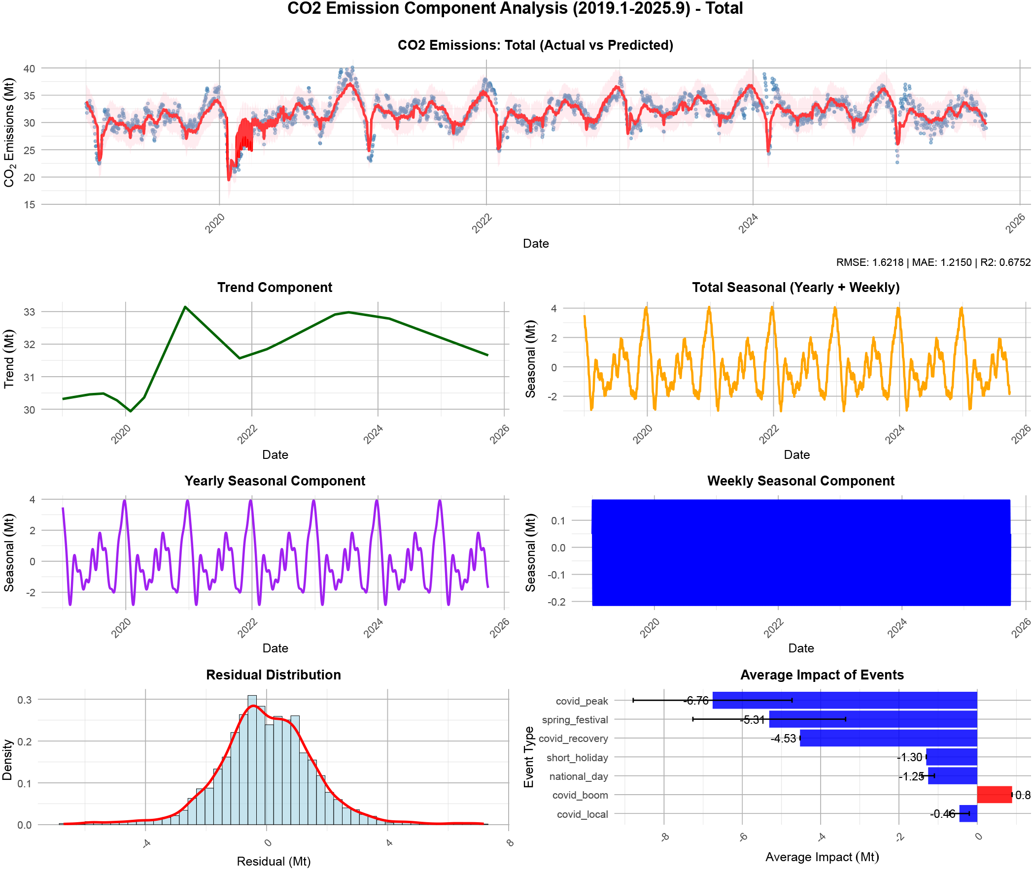
Decomposing China's daily CO2 emissions
1. Introduction
As the largest carbon emitter and second-largest economy in the world, China has proposed dual carbon goals of peaking carbon emissions before 2030 and achieving carbon neutrality before 2060. To implement differentiated emission reduction policies, it is essential to accurately capture the temporal structural characteristics of carbon emissions across various sectors. Real-time carbon emission data system covering multiple dimensions—including total emissions, industrial emissions, and power sector emissions—has been preliminarily established, providing foundational support for temporal dimension analysis. The carbon emission system exhibits trend, cyclical, and stochastic characteristics 1, influenced by multiple factors. The containment measures during the COVID-19 pandemic in 2020 led to a sharp short-term decline in emissions from aviation and industrial activities 2, whereas residential emissions underwent structural changes due to stay-at-home policies, highlighting the need to analyze the temporal structure of emissions 3. Based on real-time multisector data from China, this study constructed a Prophet model to analyze the temporal characteristics of carbon emissions and quantify the impact of the pandemic to support the optimization of emission reduction policies.
Research on carbon emission time-series analysis has evolved from aggregate studies to structural decomposition and sectoral heterogeneity 4. Recent studies have increasingly focused on fine-grained decomposition based on high-frequency data, emphasizing components such as long-term trends, seasonal cycles, and short-term fluctuations 5,6,7. For instance, Yang and O’Connell employed an autoregressive integrated moving average (ARIMA) model to analyze carbon emissions from aviation fuel 8. Huang et al. investigated carbon emissions by integrating the environmental Kuznets curve hypothesis, nonlinear multivariate grey model, and STIRPAT framework 9. Zhong et al. 10 pioneered a modified ARIMA model for analyzing daily carbon emissions. Luo et al. 11 developed a spatial simulation of urban carbon emissions by integrating multi-objective programming and principal component analysis. Models capable of explicit-series decomposition, such as Prophet, are progressively supplanting traditional econometric approaches 12. This progress has been particularly facilitated by the COVID-19 pandemic, which served as a natural experiment, revealing significant sectoral heterogeneity in the response of carbon emissions to major shocks.
The short-term suppressive effect of the COVID-19 pandemic on carbon emissions has been a prominent research focus, with existing literature primarily concentrating on quantifying the impact and elucidating the underlying mechanisms. Long et al. 13 and Wang and Su 14 documented a historic decline in CO\(_2\) emissions during the COVID-19 lockdown periods. Yadav et al. 15 used monitoring data and confirmed an approximate 30% year-on-year decrease in carbon emissions in the Los Angeles and Washington-Baltimore metropolitan areas during the 2020 lockdown. Notably, emission reductions in the ground transportation and aviation sectors substantially exceeded those in the power and industrial sectors, reflecting differential sensitivities to changes in economic activity 16. While these studies provide a foundation for analyzing the impact of sudden events on the temporal structure of carbon emissions 17, most focus on the short-term effects during the initial pandemic phase, lacking sustained tracking of the temporal evolution during the recovery stage and comparative analyses across multiple sectors.
Thus, while the academic community has made substantial progress in understanding carbon emission time series, pandemic impacts, and model applications, three critical research gaps remain. First, there is insufficient analysis of the temporal structure within real-time data; existing studies predominantly rely on annual or monthly data, limiting the ability to capture intra-day, intra-weekly, and other short-cycle dynamics 18. Second, comparative analysis of multisector emission time series before and after the pandemic is scarce, failing to systematically quantify its differential impacts. Third, the application of decomposition-based models in structural analysis is underutilized; precisely designed approaches for component decomposition and feature capture are scarce. This study contributes three key innovations:
-
・
It employs real-time data spanning six major sectors to dissect multiscale temporal characteristics—data.
-
・
It uses a major event as a nodal point to systematically compare changes in emission components and quantify their impact mechanisms—perspective.
-
・
It constructs a Prophet-based decomposition model, enhancing analytical accuracy through explicit component decomposition—method.
Regarding the decomposition methods for high-frequency daily time series, existing research provides a variety of classical paradigms. A classical decomposition method based on moving average techniques decomposes a series into trend, seasonal, and random components 19. While computationally simple, it struggles to handle nonlinear fluctuations. The seasonal-trend decomposition using locally estimated scatterplot smoothing was developed for iterative decomposition 20. Its strength lies in its ability to flexibly adapt to the time-varying characteristics of seasonality, making it particularly suitable for analyzing complex periodic patterns in daily data. Building on traditional methods, an automated decomposition framework based on state-space models was introduced 21. Through structural time-series modeling, this approach enables statistical inference and forecasting of latent components in daily series. These methods have laid a methodological foundation for extracting features from high-frequency carbon emission data, but they still exhibit limitations in explicitly modeling policy shocks and unexpected events (such as pandemics).
2. Methods
To accurately characterize trend characteristics, multiscale seasonal fluctuations, and external shock effects of daily CO\(_2\) emission data, this study decomposes the emission time series \(y_t\) (\(t=1,2,\dots,T\), where \(T\) is the sample size) into long-term trend, seasonal, holiday effect, COVID-19 shock, and random noise components within the Prophet model framework:
2.1. Long-Term Trend Components
The long-term trend of CO\(_2\) emissions is driven by macroeconomic factors such as economic growth, energy structure adjustments, and emission reduction policies, exhibiting non-stationarity and structural break characteristics. The piecewise linear trend approach of the Prophet model identifies changepoints to flexibly capture phased fluctuations in the trend, overcoming the limitations of traditional linear or fixed-curvature models. The Prophet model offers two functional forms: linear and logistic growth trends. Considering the growth constraints of CO\(_2\) emissions under policy restrictions, this study adopts a combined form of piecewise linear and logistic growth trends. The basic expression is as follows:
This formula represents a linear growth form, in which the base growth rate \(k\) and base intercept \(b\) can be time-varying adjusted through the vector \(\boldsymbol{a}(t)\) and parameters \(\boldsymbol{\delta}\) and \(\boldsymbol{\gamma}\). Specifically, \(k\) is the initial growth rate, reflecting the baseline growth rate of the trend; \(b\) is the initial offset, corresponding to the initial value of the trend at the reference time point; \(\boldsymbol{a}(t) = [a_{1}(t), a_{2}(t), \dots, a_{S}(t)]^{\mathsf{T}}\) is the indicator function vector, with \(S\) being the number of trend change points, where
This formula represents a logistic growth form with a saturation upper bound, where \(C(t)\) is the time-varying carrying capacity (i.e., the upper bound of growth), and the exponential term within the denominator also incorporates time-varying parameters to control the steepness and center position of the growth curve. \(C(t)\) is specified as a linear function of time incorporating the “Dual Carbon” policy goals: \(C(t) = c_{0} + c_{1}t\), where \(c_0\) is the initial carrying capacity and \(c_1\) is the growth rate of the carrying capacity; \(k\) is the initial growth rate, reflecting the baseline growth rate of the trend; \(b\) is the initial offset, corresponding to the initial value of the trend at the reference time point. This formula is selected when the time series exhibits S-shaped curve characteristics (initial acceleration, approximately linear growth in the middle phase, and deceleration with gradual saturation in the final phase). It is suitable for growth processes influenced by constraints such as resources, technology, or policies—for example, emission changes driven by the penetration rate of new energy vehicles, or the slow recovery of international aviation emissions constrained by capacity and demand after the pandemic.
The identification of changepoints is central to piecewise trend modeling. The Prophet model supports hybrid approaches that combine automatic detection and manual specification. Automatic detection operates by uniformly distributing 25 candidate changepoints across the first 80% of the time-series data, then screening for significant changepoints based on the characteristics of data volatility. Conversely, manual specification supplements this by incorporating major policy milestones (such as the announcement date of the “Dual Carbon” goals) and the onset date of the pandemic to designate key changepoints. To ensure the continuity of the trend function at these changepoints, the offset adjustment vector \(\boldsymbol{\gamma}\) must satisfy boundary conditions. The adjustment amount for the \(j\)-th changepoint is calculated as follows:
By adjusting the offset, the endpoint of the preceding trend segment is aligned with the starting point of the subsequent segment, preventing discontinuities in the trend function.
2.2. Nonlinear Seasonal Component
The seasonal fluctuations in daily CO\(_2\) emissions stem from cyclical patterns in production activities (such as peak and off-peak industrial production seasons) and seasonal variations in energy consumption (e.g., winter heating and summer cooling), exhibiting dual-period characteristics of annual and weekly cycles. This study employs a Fourier series to model the seasonal component, using a combination of sine and cosine functions with different frequencies to flexibly capture nonlinear periodic fluctuations:
Based on the annual and weekly cycles, the total seasonal component of carbon emissions can be formulated as a linear combination of the two.
2.3. Holiday Effect Component
The impact of holidays on CO\(_2\) emissions manifests as short-term fluctuations, with significant variations in both the intensity and duration of effects across different holidays. This study categorizes holidays into three types: the Spring Festival, National Day, and short holidays such as Labor Day and the Dragon Boat Festival. By integrating dummy variables with window functions, we quantify their dynamic effects. The model specification is as follows:
Window parameters are specified according to the characteristics of Chinese holidays: Spring Festival (\({l_{k}=3}\), \({u_{k}=7}\)), covering the prefestival production suspension for preparation and the postfestival buffer period for resuming operations; National Day (\({l_{k}=1}\), \({u_{k}=7}\)), covering the preholiday preparation and post-holiday adjustment period; and short holidays (\({l_{k}=0}\), \({u_{k}=3}\)), covering only the holiday period and the subsequent recovery day.
2.4. Shock Effect Modeling Approach
The impact of the COVID-19 pandemic on CO\(_2\) emissions has characteristics of stages and heterogeneity, manifesting as a multistage evolution of lockdown–recovery–rebound–local recurrence. Based on the development process of the pandemic, this study decomposed the shock effect into four stages and used segmented dummy variable modeling to accurately capture the emission responses to different intervention measures.
Based on the epidemic prevention and control policies and the characteristics of emission changes, four shock phases were defined:
-
(1)
The core lockdown period (January 23, 2020 – February 15, 2020): Nationwide large-scale lockdown, industrial and transportation activities sharply decreased;
-
(2)
The recovery period (February 16, 2020 – March 31, 2020): Low-risk areas gradually resumed work and production;
-
(3)
The economic rebound period (April 1, 2020 – June 30, 2020): After the nationwide lockdown was lifted, industrial activities “rebounded in retaliation”;
-
(4)
The local recurrence period (November 1, 2021 – December 31, 2021, March 1, 2022 – May 31, 2022, October 1, 2022 – November 30, 2022): Local areas upgraded their prevention and control measures.
Virtual variables for each segment were defined as follows:
2.5. Final Model Estimation Method
We employed the maximum a posteriori (MAP) estimation method to determine the model parameters. By incorporating regularization constraints into the objective function, optimal parameter estimates are obtained through numerical optimization algorithms. The full parameter vector of the model is defined as \(\boldsymbol{\Theta} = [\delta^{\mathsf{T}}, \gamma^{\mathsf{T}}, \theta_{s}^{\mathsf{T}}, \omega^{\mathsf{T}}, \phi^{\mathsf{T}}, \phi_{l}^{\mathsf{T}}]^{\mathsf{T}}\), where \(\phi\) denotes the shock intensity coefficient vector and \(\phi_{l}\) represents the lagged shock coefficient vector. The objective function is formulated as the negative log-posterior probability function, expressed as follows:
Minimizing the objective function is equivalent to solving an optimization problem with constraints. Since the objective function is a convex function, the limited-memory Broyden–Fletcher–Goldfarb–Shanno numerical optimization algorithm is used to determine the optimal parameters, \(\hat{\Theta}\). The algorithm updates the parameter vector through iterations, converging rapidly to the optimal solution using gradient information. The gradient calculation employs the automatic differentiation method to enhance computational efficiency.
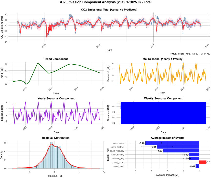
Fig. 1. CO\(_2\) emission time structure components.
3. Empirical Analysis
This study adopted the real-time daily CO\(_2\) emission data for China from January 1, 2019, to September 30, 2025, sourced from the Carbon Monitor database,(1) with the unit of MtCO\(_2\) per day. Launched in 2019, this database is a global near-real-time carbon emission database with daily-scale resolution, covering national and city-level data. The temporal structure components of China’s carbon emissions consist of seven core indicators: total emissions (Total), domestic aviation emissions (Domestic Aviation), ground transport emissions (Ground Transport), industrial emissions (Industry), international aviation emissions (International Aviation), power emissions (Power), and residential emissions (Residential). The data records are complete, with 2,465 observations, covering the entire cycle of prepandemic, pandemic, postpandemic, and recovery periods. The time structure sequence graph of China’s daily CO\(_2\) emissions is obtained by applying the methods described in Section 2, as shown in Fig. 1, with detailed analysis presented in the following subsections.
| Sector | \(R^2\) | MAPE | RMSE | MAE | Fitting quality |
| International aviation | 0.943 | 2.15 | 0.007 | 0.005 | Excellent |
| Residential | 0.922 | 3.87 | 0.206 | 0.133 | Excellent |
| Ground transport | 0.851 | 4.23 | 0.146 | 0.108 | Good |
| Power | 0.812 | 5.11 | 0.853 | 0.646 | Good |
| Domestic aviation | 0.743 | 7.26 | 0.031 | 0.023 | Good |
| Industry | 0.734 | 6.35 | 0.945 | 0.703 | Reliable |
| Total emissions | 0.675 | 3.90 | 1.623 | 1.216 | Reliable |
3.1. Model Decomposition and Error Evaluation
Four core indicators were adopted to evaluate the model fitting performance, with their definitions and calculation formulas presented as follows.
Coefficient of determination (\(R^2\)): It reflects the ability of the model to explain the variation of the emission series, with a value range of \([0,1]\). The closer the value is to 1, the higher the fitting quality. The formula is as follows:
Mean absolute percentage error (MAPE): It measures the magnitude of relative errors. Presented in percentage form, it facilitates horizontal comparison, and a smaller value indicates a lower error. The formula is as follows:
Root mean square error (RMSE): It reflects the degree of dispersion of errors and is sensitive to extreme values, with a unit consistent with that of the emission data. The formula is as follows:
Mean absolute error (MAE): It measures the average level of errors and has strong resistance to the interference of extreme values. The formula is as follows:
The evaluation results of the errors are shown in Table 1.
Table 1 shows that the overall fitting performance of CO\(_2\) emissions across all sectors is excellent. It manifests in three aspects: First, the overall fitting quality presents a clear hierarchical structure. The international aviation (\({R^{2}=0.943}\)) and residential sectors (\({R^{2}=0.922}\)) achieve the “Excellent” grade, indicating that the CO\(_2\) emission time series have stable structures and clear fluctuation patterns. The ground transport, power, and domestic aviation sectors reach the “Good” grade, in which seasonal and impact effects are accurately captured; the industry and total emissions sectors are rated as “Reliable” owing to their large scales or error accumulation; however, they still meet the requirements of the analysis. Second, the error control is precise. The MAPE of all sectors falls within the range of 2%–8%, and the MAPE of international aviation is only 2.15%, reflecting the ability of the model to fit stable sequences; the MAPE of total emissions is 3.90%, indicating that the overall estimation of the model is reliable. Third, regarding the residual test, it can be seen from the normal plot that the residuals follow an approximately normal distribution. This indicates that the model has completely decomposed structural components such as trends, seasonality, and impacts, and the remaining errors are random disturbances, verifying the reliability of the fitting results.
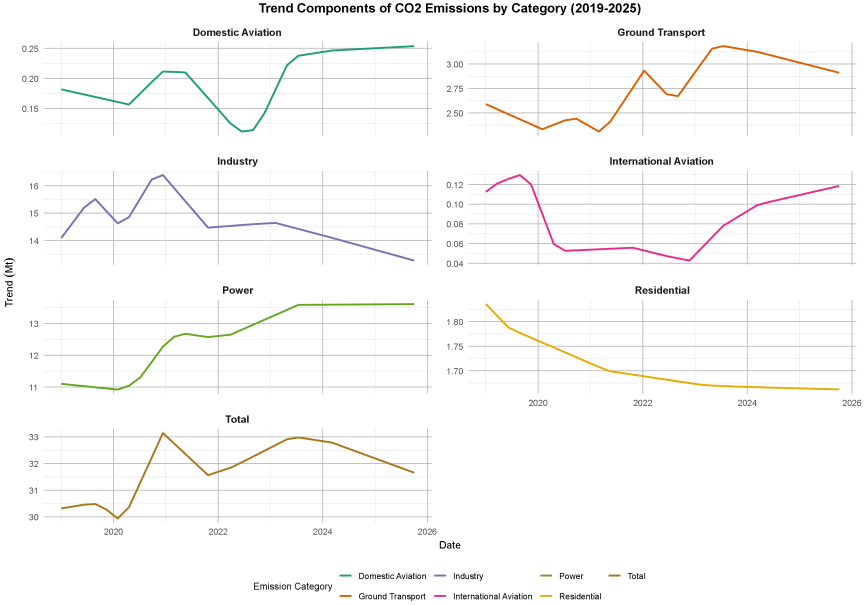
Fig. 2. Time series of trend components.
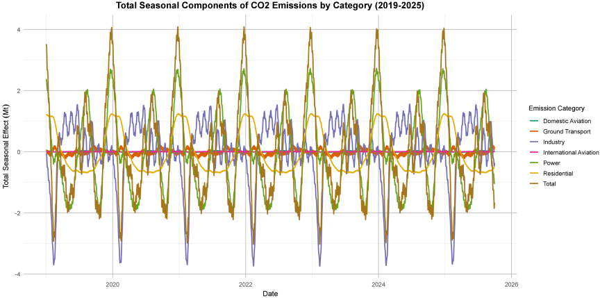
Fig. 3. Time series of seasonal components.
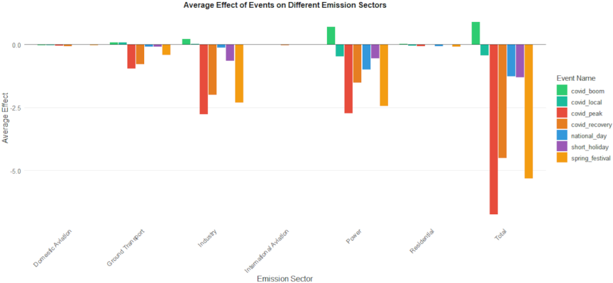
Fig. 4. Classification effect of event impact on emissions.
3.2. Analysis of Trend and Seasonal Components
Combined with the emission analysis graphs in relevant fields, the total CO\(_2\) emissions of China from 2019 to 2025 show phased evolution characteristics. From 2019 to the beginning of 2020, emissions maintained a stable change, reflecting the normal state of economic activities and energy consumption before the pandemic. At the beginning of 2020, affected by pandemic prevention and control measures, emissions experienced a phased decline, corresponding to the phased adjustment of industrial production and transportation activities. From the middle of 2020 to 2021, emissions gradually recovered, reflecting the recovery of economic and social activities. After 2022, emissions showed a steady downward trend, which became more pronounced after March 2024, related to the implementation effects of policies such as the increase in the proportion of non-fossil energy consumption and emission reduction in key industries.
As shown in Fig. 2, from a sectoral perspective, as the main source of emissions, the fluctuation of industrial emissions is highly correlated with the adjustment of production activities. After a significant decline at the beginning of 2020 due to pandemic disruptions, it gradually recovered alongside the resumption of work and showed a stable trend after 2022 with the optimization of industrial structure and energy consumption control, reflecting the effectiveness of the green transition policies of China. The emission scale of the power sector remains at a high level, maintaining relative stability from 2021 to 2022, and showing a slow downward trend after 2023 due to the adoption of clean energy such as wind and photovoltaic power.
In the transport sector, the domestic aviation emissions fluctuate significantly under the influence of changes in travel demand, gradually recovering after a sharp decline at the beginning of 2020 and tending to stabilize after 2024. The recovery of international aviation emissions is relatively slow and slower than that of domestic aviation. The overall fluctuations of ground transport emissions are gentle, maintaining stability after 2023 with the promotion and application of new energy vehicles. The emission trend of the residential sector is the most stable, less affected by external factors, showing a slow overall change characteristic.
The divergence in recovery patterns between domestic and international aviation underscores the varying sensitivity of transport subsectors to global mobility restrictions and economic reopening phases, while the stabilization in ground transport highlights the gradual decarbonization effect of vehicle electrification policies.
As shown in Fig. 3, there are clear differences in seasonal characteristics between various sectors. The residential sector has the most prominent seasonal fluctuations, showing a double-peak feature of high in winter, secondarily high in summer, and low in spring and autumn. Emissions rise significantly in winter due to heating demand and increase again in summer because of cooling demand, reflecting the strong driving effect of climate factors on residential energy consumption. The seasonality of the power sector is largely consistent with that of the residential sector, also presenting a double-peak in winter and summer. The increase in power generation demand in summer and winter is affected by the dual seasonal fluctuations of residential energy consumption and industrial production, naturally leading to a corresponding rise in emissions. The ground transport sector shows certain seasonal fluctuations as well, with relatively concentrated travel activities in spring and autumn, resulting in comparatively higher emissions during these seasons. Additionally, a clear weekly characteristic is that emissions on weekends are higher than those on weekdays, which is closely related to the concentrated leisure travel demand. The seasonal fluctuations of the industry sector are relatively mild. Affected by production plans and holiday arrangements, emissions are relatively low in winter and spring, and relatively high in summer and autumn. The aviation sectors have generally weak seasonal characteristics, and the seasonal fluctuations during the pandemic are even more gentle, which are slightly apparent only after 2023 with the gradual recovery of travel demand.
3.3. Analysis of Holiday and COVID-19 Event Impact Effects
Figure 4 presents the event impact effects of holidays and COVID-19 on carbon emissions. As shown in Fig. 4, there are significant differences in the extent and direction of the impact of the two types of events (COVID-19 pandemic and holidays) on CO\(_2\) emissions across various industrial sectors. These differences are determined not only by the regulatory attributes of the events but also by the core driving factors of carbon emissions in each sector.
Impact Effect of the COVID-19 Pandemic on CO2 Emissions: The intensity of prevention and control measures at different stages of the pandemic directly determines the fluctuation range of industrial emissions. During the “covid peak” (pandemic peak period), emissions of all sectors experienced severe negative fluctuations under nationwide regulatory measures: the average impact on total emissions reached \(-7\), and the negative impacts on the industry and power sectors exceeded \(-2.5\). This result stems from the fact that industry and power are the core sources of carbon emissions, with their operational scale highly reflective of emission levels. The complete suspension of production activities directly led to a sharp reduction in emissions. Entering the “covid recovery” (pandemic recovery period), prevention and control measures were marginally relaxed, but industrial production had not yet returned to normal scale, and emissions still showed negative fluctuations, albeit with a lower intensity than during the peak period.
In the “covid boom” (post-pandemic rebound period), pandemic control measures were fully lifted, and the rebound of industrial production demand resulted in the effect of the impact on total emissions and the power sector approaching zero or even turning positive, confirming the direct driving effect of the operational flexibility of high-emission sectors on emissions. In contrast, the impact of “local covid” (local pandemic resurgences) was relatively moderate, with the negative effect on most sectors being less than \(-0.5\). This is because local control measures only targeted specific regions and did not form an overall constraint on the operation of the entire industry, thus limiting the range of emission fluctuations.
Impact Effect of Holidays on CO2 Emissions: The intensity of the impact of holidays on emissions is jointly determined by the duration of the holiday and the mode of social operation adjustment. As a national long holiday, the Spring Festival has the most significant impact on emissions: the negative impacts on the industry and power sectors exceeded \(-2.5\), and the negative effect on total emissions reached more than \(-5\). This is due to the centralized shutdown of industrial production during the Spring Festival, as the suspension of production activities led to a substantial decline in electricity demand, resulting in a significant contraction in emissions. In contrast, the impact intensity of the National Day and short holidays is significantly weaker: the negative effect on most sectors is less than \(-0.5\), and the impact on sectors such as international aviation is even closer to zero. The reason lies in the short duration of these holidays and their focus on consumption-oriented activities, which do not form sustained interference with industrial production. The continuity of industrial operation remains unbroken, thus limiting fluctuations in emission levels.
Heterogeneity of Sectoral Responses: The sensitivity of each sector to the impacts of the two types of events is directly related to the driving logic of its carbon emissions. The industry and power sectors exhibit the highest sensitivity: whether it is production suspension under pandemic control or centralized shutdown during the Spring Festival holiday, their negative emission fluctuations are the highest in all sectors. This is rooted in the fact that their emissions are completely dependent on production scale, and interventions in production rhythms are synchronously transmitted to emission changes. The ground transport sector ranks second in sensitivity, with a negative impact close to \(-\)2.5 during the pandemic peak period. This is because transportation emissions are directly linked to the scale of population mobility, and mobility restrictions under pandemic control quickly trigger emission fluctuations. In contrast, the impact on domestic aviation, international aviation, and residential sectors is generally weak: the aviation industry has a small emission base, and residential sector emissions are mainly driven by essential living needs. The two types of events have limited interference with their operational scales, resulting in relatively stable emission levels.
Comparative Analysis of the Impacts of the Two Types of Events: The impact of the pandemic on emissions is characterized by its mandatory nature and nationwide coverage, with an intensity far higher than that of holidays. In contrast, the impact of holidays is periodic and local, only adjusting the operational rhythm of specific sectors. This difference not only reflects the disparity in intervention intensity between emergent events and regular social rhythm changes on industrial operations but also provides a reference for the dynamic management of carbon emissions. Although the pandemic can suppress emissions in the short term, it is accompanied by the economic cost of industrial shutdowns. In contrast, emission fluctuations during holidays reflect the natural regulation of social operation rhythms on emissions. This type of regulation incurs no additional costs and is one of the core sources of seasonal fluctuations in carbon emissions.
4. Conclusions and Prospects
Based on the Prophet framework, this study systematically decomposes the time structure components of the daily CO\(_2\) emissions of China from 2019 to 2025. Through the hierarchical modeling of the long-term trend term, nonlinear seasonal component, holiday effect term, and COVID-19 impact term, combined with MAP estimation and regularization constraints, the multidimensional characteristics of the emission series are accurately depicted. The core conclusions are as follows:
First, the model is scientifically constructed and exhibits excellent fitting accuracy. The trend term integrating piecewise linear and logistic growth, the dual-cycle seasonal component fitted by a Fourier series, and the event impact term characterized by piecewise dummy variables form a complete emission structure decomposition system. Multidimensional error evaluation indicates that the fitting quality grades of the international aviation and residential sectors reach “Excellent,” while the remaining sectors are rated as “Good” or “Reliable.” The MAPE of all sectors is within the range of 2%–8%, and the residuals follow an approximately normal distribution, verifying the ability of the model to capture the laws of emission fluctuations.
Second, the temporal structure characteristics of emissions show significant phase and sectoral heterogeneity. In terms of long-term trends, total emissions present a steady downward trend after 2022. The industry and power sectors are significantly driven by the “dual carbon” policy and energy structure adjustment; the transport sector exhibits phased recovery characteristics with the restoration of travel demand; and the residential sector shows the most stable emission trend. Regarding seasonality, the residential and power sectors display a double-peak feature (higher in winter, secondarily higher in summer, and lower in spring and autumn). Fluctuations in ground transport are consistent with travel demand patterns, whereas the aviation sectors have weak seasonal characteristics.
Third, the event impact effects are significantly differentiated. The mandatory and nationwide impact of the COVID-19 pandemic is far stronger than the periodic and local impact of holidays. The peak period of the pandemic exerts the most severe negative impact on total emissions as well as the industry and power sectors, whereas the impact of local COVID-19 outbreaks is relatively moderate. Of the holidays, the Spring Festival has a stronger inhibitory effect on emissions than the National Day and short holidays, primarily due to the centralized shutdown of industrial production. In terms of sectoral responses, the industry and power sectors are the most sensitive to both types of events, while the domestic aviation, international aviation, and residential sectors show lower sensitivity. This difference stems from the inherent variations in the emission-driven logic of each sector.
Future research can be further deepened and expanded in two aspects. First, the model setting may be optimized by incorporating more refined policy nodes and energy market price factors into the trend term and introducing meteorological factor interaction terms into the seasonal component to enhance the explanatory power of the model under complex driving mechanisms. Second, the application orientation may be strengthened. Based on the structural decomposition results of this study, short-term carbon emission prediction models and scenario simulation tools may be constructed to provide more operable technical support for the formulation of differentiated emission reduction policies and dynamic management of key sectors, facilitating the scientific implementation and long-term advancement of the “dual carbon” goals.
Acknowledgments
We would like to thank the reviewers for their valuable comments and suggestions that helped improve the quality of the paper.
Footnotes
(1) https://www.carbonmonitor.org.cn/ [Accessed November 17, 2025]
- [1] S. Qu and C. Guo, “Forecast of China’s carbon emissions based on STIRPAT modely,” China Popul. Resour. Environ., Vol.20, No.12, pp. 10-15, 2010 (in Chinese).
- [2] C. Yan et al., “Impacts of COVlD-19 traffic control policy on population flows in Changsha,” J. Transp. Syst. Eng. Inf. Technol., Vol.21, No.5, pp. 190-197, 2021 (in Chinese). https://doi.org/10.16097/j.cnki.1009-6744.2021.05.019
- [3] F. Dong et al., “Drivers of carbon emission intensity change in China,” Resour. Conserv. Recycl., Vol.129, pp. 187-201, 2018. https://doi.org/10.1016/j.resconrec.2017.10.035
- [4] L.-C. Liu, Y. Fan, G. Wu, and Y.-M. Wei, “Using LMDI method to analyze the change of China’s industrial CO2 emissions from final fuel use: An empirical analysis,” Energy Policy, Vol.35, No.11, pp. 5892-5900, 2007. https://doi.org/10.1016/j.enpol.2007.07.010
- [5] J. Jiang, C. Han, W. X. Zhao, and J. Wang, “PDFormer: Propagation delay-aware dynamic long-range transformer for traffic flow prediction,” Proc. AAAI Conf. Artif. Intell., Vol.37, No.4, pp. 4365-4373, 2023. https://doi.org/10.1609/aaai.v37i4.25556
- [6] H. Qin and M. Han, “Real-time forecasting and short-term prediction of Chinese carbon dioxide emissions based on MIDAS model,” Acta Sci. Circumstantiae, Vol.38, No.5, pp. 2099-2107, 2018 (in Chinese). https://doi.org/10.13671/j.hjkxxb.2017.0496
- [7] Y. Jiang et al., “Dynamic carbon emission responsibility factor of electricity,” Proc. CSEE, Vol.44, No.17, pp. 7024-7039, 2024 (in Chinese). https://doi.org/10.13334/j.0258-8013.pcsee.240573
- [8] H. Yang and J. F. O’Connell, “Short-term carbon emissions forecast for aviation industry in Shanghai,” J. Clean. Prod., Vol.275, Article No.122734, 2020. https://doi.org/10.1016/j.jclepro.2020.122734
- [9] S. Huang, X. Xiao, and H. Guo, “A novel method for carbon emission forecasting based on EKC hypothesis and nonlinear multivariate grey model: Evidence from transportation sector,” Environ. Sci. Pollut. Res., Vol.29, No.40, pp. 60687-60711, 2022. https://doi.org/10.1007/s11356-022-20120-5
- [10] W. Zhong et al., “Accurate and efficient daily carbon emission forecasting based on improved ARIMA,” Appl. Energy, Vol.376, Part A, Article No.124232, 2024. https://doi.org/10.1016/j.apenergy.2024.124232
- [11] H. Luo et al., “Carbon emission prediction model of prefecture-level administrative region: A land-use-based case study of Xi’an city, China,” Appl. Energy, Vol.348, Article No.121488, 2023. https://doi.org/10.1016/j.apenergy.2023.121488
- [12] X. Zeng and Y. Zhao, “Study on the application of LSTM network in subway tunnel subsidence prediction,” J. Gansu Sci., Vol.31, No.6, pp. 117-122, 2019 (in Chinese). https://doi.org/10.16468/j.cnki.issn1004-0366.2019.06.021
- [13] Y. Long et al., “Japanese urban household carbon footprints during early-stage COVID-19 pandemic were consistent with those over the past decade,” npj Urban Sustain., Vol.3, Article No.19, 2023. https://doi.org/10.1038/s42949-023-00095-z
- [14] Q. Wang and M. Su, “A preliminary assessment of the impact of COVID-19 on environment – A case study of China,” Sci. Total Environ., Vol.728, Article No.138915, 2020. https://doi.org/10.1016/j.scitotenv.2020.138915
- [15] V. Yadav et al., “The impact of COVID-19 on CO2 emissions in the Los Angeles and Washington DC/Baltimore metropolitan areas,” Geophys. Res. Lett., Vol.48, No.11, Article No.e2021GL092744, 2021. https://doi.org/10.1029/2021GL092744
- [16] J.-P. Zhang, Y.-C. Qin, Y. Zhang, and L.-J. Zhang, “Measurement of urban CO2 emission structure and low-carbon standard – A case study for Bejing, Tianjin, Shanghai and Chongging City,” Sci. Geogr. Sin., Vol.30, No.6, pp. 874-879, 2010 (in Chinese). https://doi.org/10.13249/j.cnki.sgs.2010.06.874
- [17] R. Li and S. Li, “Carbon emission post-coronavirus: Continual decline or rebound?” Struct. Change Econ. Dyn., Vol.57, pp. 57-67, 2021. https://doi.org/10.1016/j.strueco.2021.01.008
- [18] X. Dou et al., “Near-real-time global gridded daily CO2 emissions 2021,” Sci. Data, Vol.10, Article No.69, 2023. https://doi.org/10.1038/s41597-023-01963-0
- [19] D. M. Miller and D. Williams, “Shrinkage estimators of time series seasonal factors and their effect on forecasting accuracy,” Int. J. Forecast., Vol.19, No.4, pp. 669-684, 2003. https://doi.org/10.1016/S0169-2070(02)00077-8
- [20] R. B. Cleveland, W. S. Cleveland, J. E. McRae, and I. Terpenning, “STL: A seasonal-trend decomposition procedure based on loess,” J. Off. Stat., Vol.6, No.1, pp. 3-73, 1990.
- [21] D. F. Findley, B. C. Monsell, W. R. Bell, M. C. Otto, and B.-C. Chen, “New capabilities and methods of the X-12-ARIMA seasonal adjustment program,” J. Bus. Econ. Stat., Vol.16, No.2, pp. 127-152, 1998. https://doi.org/10.1080/07350015.1998.10524743
This article is published under a Creative Commons Attribution-NoDerivatives 4.0 Internationa License.