
Research Paper:
MRI Imaging Recognition Model for Spinal Lesions Based on Multiple Attention Mechanism
Hui Zhou*,†
 , Hong Zhu*
, Xinjing Song*, Peng Chen**,†
, Yuan Wang***,†
, and Xiangji Liu***
*School of Software, Dalian Neusoft University of Information
No.8 Software Park Road, Ganjingzi District, Dalian, Liaoning 116023, China
**Navigation College, Dalian Maritime University
No.1 Linghai Road, Dalian, Liaoning 116026, China
***The Second Affiliated Hospital, Dalian Medical University
No.467 Zhongshan Road, Shahekou District, Dalian, Liaoning 116044, China
†Corresponding author

Manual detection of spinal pathologies is a labor-intensive process that relies heavily on clinical expertise; thus the development of automated identification systems is clinically imperative. However, distinguishing among spinal lesions—specifically spinal tumors, spinal brucellosis (a rare infectious disease), and spinal tuberculosis—presents a significant challenge due to their high radiological mimicry. These conditions share overlapping imaging features, including vertebral bone destruction, intervertebral space narrowing, and paravertebral soft tissue swelling. Furthermore, the extent of the lesions and the specific vertebral segments involved lack fixed patterns, leading to frequent feature confusion. To address these issues, we propose an improved computational framework. Firstly, we introduce a bidirectional feature pyramid network backbone based on ResNet-101. Deformable convolution is employed instead of traditional convolution across various layers to extract richer semantic features. Concurrently, multiple attention mechanisms, including self-attention and soft attention, are integrated into different modules to effectively fuse the most informative feature components. Finally, an improved balanced cross-entropy loss function is implemented to mitigate the data imbalance issue arising from the rarity of both spinal tumors and brucellosis. The proposed model was validated on a clinical dataset comprising MRI images from 135 patients. Experimental results demonstrate that the model outperforms other classical models in multiple core performance metrics. Specifically, the model achieved an accuracy of 96.6%, precision of 94.2%, recall of 90.8%, and an F1-score of 92.5%. This work provides reliable technical support for the precise diagnosis of spinal tumors, spinal brucellosis, and spinal tuberculosis.
1. Introduction
Spine lesions are abnormal areas appearing in or around spinal tissues. These lesions can arise from various causes, including tumors, infections, or other rare conditions. As different diseases often present with highly similar imaging features, the accurate identification of spinal lesions is a critical step in diagnosing and treating spinal conditions, directly impacting patient prognosis and quality of life.
MRI is a non-invasive modality for examining spinal lesions 1. Compared to CT and PET, MRI offers sensitive information through multiple sequences—typically T1-weighted, T1 contrast-enhanced, T2-weighted, and FLAIR. This rich dataset facilitates more reliable and efficient lesion identification, making MRI a preferred tool for evaluating suspicious spinal lesions prior to other medical interventions.
Current MRI image recognition methods for spinal lesions broadly fall into two categories: (1) traditional methods reliant on manual interpretation by clinicians; and (2) artificial intelligence (AI) methods leveraging computer-aided recognition. Manual interpretation methods depend heavily on the clinician’s years of diagnostic experience and their ability to discern lesion characteristics visible to the naked eye in MRI images. This approach can lead to over-reliance on subjective judgment and may suffer from lower efficiency and variable accuracy. In contrast, early AI-based, computer-assisted methods involved extracting image features and then applying classic classification algorithms—such as K-nearest neighbors (KNN), support vector machines (SVM), naïve Bayes, and decision trees—for lesion recognition 2.
More recently, deep learning has become widely adopted in computer vision, particularly for image classification, achieving breakthrough successes. It offers powerful auxiliary capabilities for the rapid diagnosis and identification of diseases. Deep learning models are structured to mimic the neural connections of the human brain. These models can accurately extract key hierarchical features from images, from low-level to high-level, effectively describing and interpreting detected information. This allows for the exploration of deeper, more nuanced feature information within images, leading to more accurate and efficient lesion identification 3.
Currently, deep learning recognition models have demonstrated promising results in identifying various cancers, including prostate, breast, lung, and craniocerebral tumors 4,5,6. For instance, Li and Ping 7 proposed a fusion of a convolutional neural network (CNN) model with a fully connected conditional random field, achieving improved visual effects in image block prediction. Shao et al. 8 introduced a multi-scale block enhancer to address the challenge of effectively detecting small tumor areas. Sharif et al. 9 utilized a dataset of 3064 T1-weighted contrast-enhanced MRI images to identify various brain cancers, including gliomas, meningiomas, and pituitary tumors, achieving 94% accuracy. Coburger et al. 10 proposed a fully automated three-dimensional cellular neural network model for the low- and high-grade classification of brain gliomas, employing pre-processing methods such as grayscale normalization and adaptive contrast enhancement.
Spinal lesions exhibit a wide range of radiologic characteristics, with features such as location, structure, size, and shape varying considerably among patients, leading to high heterogeneity. To improve the diagnosis of these lesions, many researchers are exploring the application of deep learning models. For instance, Lang et al. 11 employed dynamic contrast-enhanced MRI in 61 patients with no prior tumor history, utilizing a CNN model to differentiate spinal metastases. This approach achieved an accuracy of 81%, demonstrating considerable efficacy in diagnosing this condition. In other work, Chianca et al. 12 developed both binary and tri-class classification models for spinal tumors using deep learning methods. Their findings indicated that a deep CNN yielded the best binary classification performance, with accuracy exceeding 90%. However, the tri-class model was less effective, likely due to the pronounced heterogeneity of spinal tumors. Diniz et al. 13 proposed a model incorporating dense connections with residual learning, which enhanced feature information learning and improved spinal tumor detection. Furthermore, Li et al. 14 evaluated various architectures (ResNet-18/50, VGG-11/16, and DenseNet-121/161) for diagnosing spinal tuberculosis, reporting that the VGG-11 network achieved optimal performance across accuracy, AUC, sensitivity, and specificity. Additional studies by Chianca et al. 12 and Arends et al. 15 also applied multi-scale CNN and D-CNN models, respectively, to the classification and identification of spinal lesions.
In clinical diagnosis, accurately identifying intravertebral lesions in MRI images is challenging due to the inherent limitations of human visual acuity. Distinguishing between conditions such as spinal tumors, tuberculosis, and rarer diseases like brucellosis can be particularly difficult 16,17. Furthermore, diagnostic accuracy is often constrained by varying levels of clinical experience, increasing the likelihood of misjudgment when identifying spinal lesions. To address these challenges, we propose a novel recognition model based on a multi-attention mechanism designed to differentiate among spinal tumors, brucellosis, and tuberculosis. Since these conditions exhibit high radiological mimicry with overlapping features, such as vertebral bone destruction, intervertebral space narrowing, and paravertebral soft tissue swelling, our model incorporates a bidirectional feature fusion backbone and deformable convolutional networks (DCN). These components effectively extract subtle discriminative features of vertebral destruction and soft tissue swelling across multiple scales, while precisely capturing the morphology and boundaries of irregular, heterogeneous lesions to reduce feature confusion. Furthermore, to mitigate class imbalance, especially regarding the scarcity of samples for spinal tumors and brucellosis, we employ a dual mechanism combining self-attention and soft attention. This approach enhances feature representation for minority classes through global feature interaction and simultaneously focuses on critical lesion regions while suppressing irrelevant background noise. Experimental results demonstrate that the proposed model improves the identification accuracy of spinal lesion-associated diseases.
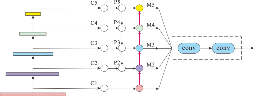
Fig. 1. Multi-feature converged backbone network.
2. Materials and Methods
2.1. Backbone Network
The proposed active identification model for spinal lesions utilizes a multi-feature fusion backbone network. This network integrates features from various scales within the deep architecture, drawing inspiration from the feature pyramid network (FPN) 18, a common multi-scale fusion model. The backbone initially generates feature map layers C1–C5 in a bottom-up manner. Then, layers C2 through C5 are processed: each is subjected to a \({1\times 1}\) convolution (outputting 256 channels) via a lateral connection to its corresponding backbone feature map. This yields the new feature maps P2, P3, P4, P5, as specified in Eq. (1):
A recognized limitation of conventional FPN is the potential for information degradation during upsampling and downsampling. Given that the robust identification of spinal lesions mandates the extraction of comprehensive multi-layer features, this work adopts an enhanced Bi-directional FPN (BiFPN) as its backbone. The bidirectional architecture of BiFPN facilitates the concurrent capture of high-level micro-structural attributes and low-level organ-scale morphological features. Such two-way hierarchical linking enables the derivation of highly discriminative features, even under conditions of limited training data, particularly for rare pathologies. In contrast to alternative multi-feature fusion paradigms like NAS-FPN, which necessitate substantial volumes of high-quality annotated data, BiFPN demonstrates superior applicability to scenarios characterized by medical data limitations and the paucity of labeled samples for rare diseases. Specifically, BiFPN leverages the P2 feature map from the initial FPN structure as the starting point for a new bottom-up pathway. It then iteratively fuses features from the current layer with those of the preceding layer, progressing upwards to the P5 layer, thereby generating an augmented set of multi-scale feature maps M2, M3, M4, and M5 (depicted in Fig. 1). The establishment of bidirectional connections between the top-down and bottom-up pathways permits feature amalgamation in both directions, thus enabling a more efficacious synthesis of salient multi-scale features. Subsequent computations, predicated on Eq. (1), are elaborated in Eq. (2):
The multi-feature fusion network initially employs standard convolution kernels for its feature mapping layers. However, standard convolution utilizes a fixed, rigid receptive field, which limits its adaptability to the diverse shapes and scales of target objects. This inherent inflexibility can reduce convolutional efficiency, particularly when dealing with irregularly shaped targets. To address this, we incorporate deformable convolution, which enhances the network’s ability to model geometric transformations. Unlike standard convolution, deformable convolution introduces learnable 2D offsets to the regular grid sampling locations within the convolution kernel. This allows the sampling grid to dynamically adapt to the target’s structure, effectively creating a flexible receptive field. Consequently, deformable convolution can achieve superior local feature enhancement and significantly alleviate the problem of intraclass variability often encountered in medical images. Furthermore, its stronger small-sample learning capability is particularly advantageous when training models on datasets with limited volume, such as those for rare diseases.
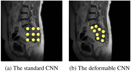
Fig. 2. Comparison with the standard CNN and the deformable CNN.
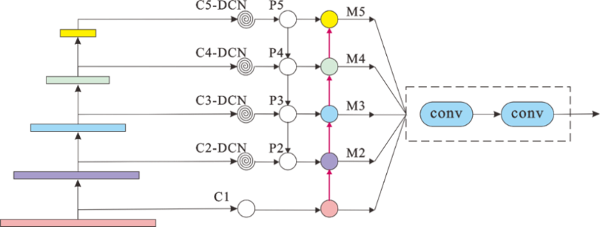
Fig. 3. Multi-feature fusion network structure diagram.
To more effectively extract salient lesion features, we replace the standard convolution kernels in the convolutional layers C2, C3, C4, and C5 of our network with deformable convolution kernels. Specifically, for an input feature map, an additional parallel convolutional layer learns these 2D offsets for each sampling point of the standard convolution kernel. If the input feature map has \(N\) channels, this offset-generating layer outputs \(2N\) channels, where the two dimensions correspond to the \(\Delta x\) and \(\Delta y\) offsets for each of the \(N\) channels at every spatial location. As illustrated in Fig. 2, during the training process, both the weights of the main convolution kernel (used to generate output features) and these spatial offsets are learned simultaneously via backpropagation. Bilinear interpolation is typically used to compute the feature values at the (often fractional) offset locations from the input feature map:
Here, \(w\) is the network weight parameter, \(\Re\) is the specified convolution area, and \(p_{n}\) is the position offset learned on ordinary convolution. On the basis of the position of ordinary convolution, a learning position offset \(\Delta p_{n}\) is added, so the formula for variable kernels to convert convolution is as follows:
Here, \(\Delta p_n\) is a learnable floating-point parameter. During the forward pass, bilinear interpolation is employed to compute feature values at non-integer sampling locations. The objective of backpropagation is to compute the gradients of the loss function with respect to the offsets \(\Delta p_n\), which are then used to update these offsets. Specifically, the gradient calculation follows the chain rule: the gradient of the loss with respect to the deformable convolution output \(y(p_{0})\) is computed first, followed by the computation of the gradient of the output with respect to the offsets.
Deformable convolution, by offsetting its convolutional kernels, adaptively adjusts their shapes based on the input features, enabling more effective extraction of image characteristics. The adoption of DCN can enhance the feature representation capabilities of image object detection networks. Fig. 3 illustrates the optimized backbone network.
Furthermore, the hyperparameters for the DCN have been specified: the kernel size for layers C2–C5 is set to \({3 \times 3}\) with a stride of 1 to preserve the spatial dimensions of the feature maps. The number of feature channels is standardized at 256. Regarding feature integration, an L1-normalized weight fusion method was adopted, as it is particularly suitable for lesion diagnosis.
2.2. Multiple Attention Mechanism Module
Spinal lesions such as spinal tumors, tuberculosis, and brucellosis are difficult to distinguish due to many interferences in MRI. In order to improve the ability of features to express images, different attention mechanisms are adopted for different feature mapping layers in the multi-feature fusion backbone network.
2.2.1. Transform Attention Component
The Transformer is a model architecture primarily leveraging self-attention mechanisms, typically composed of multiple encoder and decoder stacks. It utilizes multi-head attention to capture global dependencies between different positions within the input and output sequences. The model processes input data, such as feature maps (often flattened into one-dimensional sequences) or token embeddings, which are combined with positional encodings and then fed into the encoder. Within the encoder, multi-head self-attention mechanisms enable each element in the sequence to weigh the importance of all other elements, thereby extracting contextually rich representations. This focus on the overall input information allows the model to emphasize relevant features or “target” areas while reducing interference from less pertinent background elements 19.
The Transform Attention Component (TAC), leveraging the Transformer’s self-attention mechanism, is particularly vital for detecting lesions in MRI scans. Its effectiveness stems from its ability to compute attention weights for all entities within an input feature layer. This process selectively amplifies the attention weights of target lesions while concurrently down-weighting those of other interfering tissues or anatomical structures. Unlike contemporary attention models such as CBAM or SE-Net, the integration of the TAC module, with its self-attention operations executed at lower architectural levels (e.g., within a multi-stage attention design), offers superior capabilities for discerning organ-level morphological characteristics. In essence, TAC processes an input feature sequence by projecting it through different learnable weight matrices to derive the Query (\(Q\)), Key (\(K\)), and Value (\(V\)) matrices. The Query matrix can be conceptualized as representing the input features themselves, against which the Key matrix (derived from the same input features) is compared to determine attention scores, and the Value matrix (also derived from the input) provides the information to be aggregated.
Here, \(W_{q}\), \(W_{k}\), and \(W_{v}\) are distinct learnable weight matrices. The attention matrix is computed by taking the matrix product of the query matrix (\(Q\)) and the key matrix (\(K\)), followed by the application of a softmax function. To achieve a weighted aggregation of values, this attention matrix is then multiplied by the value matrix (\(V\)). The result of this operation represents the captured relationships among lesions in the MRI images. Finally, this mechanism is extended to multi-head attention within the TAC module, as formulated in Eq. (6):
Here, \(M\) is the number of attention heads and \(d_{k}\) is the dimensionality of \(K\). In the backbone’s feature extraction phase, the TAC module processes the final P5 feature map. By leveraging a self-attention mechanism, the module models inter-regional relationships to capture global contextual information and learn long-range spatial dependencies. This transforms the input into a more expressive feature representation, as depicted in Fig. 4.
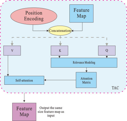
Fig. 4. TAC component.
2.2.2. Soft Attention Component
To improve feature expressiveness, we integrate a soft attention component (SAC) to model inter-channel dependencies within the multi-scale feature maps of our fusion backbone. The SAC module first aggregates spatial information by applying parallel global average pooling and global max pooling to the input feature map \(\boldsymbol{F}\) (\({H \times W \times C}\)), yielding two distinct channel descriptors: \(\boldsymbol{F}_{\mathrm{avg}}\) and \(\boldsymbol{F}_{\mathrm{max}}\) (both \({1 \times 1 \times C}\)). These descriptors are then fed into a shared two-layer multi-layer perceptron (MLP), referred to as TFC, to capture complex channel-wise relationships. The output vectors from the MLP are merged and activated by a sigmoid function to generate the final channel attention vector \(\boldsymbol{\omega}\). This vector is then used to re-calibrate the original feature map \(\boldsymbol{F}\) via channel-wise multiplication, producing a feature map with selectively enhanced channels, as depicted in Fig. 5.
To enhance model accuracy while maintaining computational efficiency, we introduce a flexible multi-attention mechanism into the M2–M4 modules. As illustrated in Fig. 6, this mechanism enables the model to selectively fuse the most salient features, thereby focusing on the most informative parts of the feature map.
Figure 6 presents a full architecture diagram. Specifically, MRI slices from axial and sagittal views were treated as independent samples and fed into the model. The model architecture enables the separate learning of different features from the axial and sagittal views. This architecture is designed to effectively capture subtle discriminative features of vertebral destruction and soft tissue swelling across multiple scales. Furthermore, by incorporating the multi-attention mechanism, the model enhances both the specificity and precision of feature extraction for complex pathological lesions.
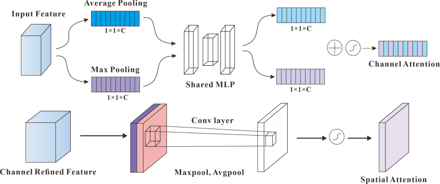
Fig. 5. SAC component.
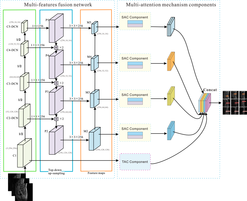
Fig. 6. A full architecture diagram.
2.3. Loss Function Design
For multi-class classification tasks, the cross-entropy (CE) loss \(\mathrm{L}_{ce}(p_{i})= {-\ln p_{i}}\) is a commonly used function, where \(p_{i}= (p_{0}, p_{1}, \dots, p_{k})\) denotes the predicted probability for class \(k\). In this study, our objective is to classify spinal lesions into three distinct categories: tuberculosis, spinal tumors, and brucellosis. A significant challenge in this task is the inherent class imbalance in the dataset, which leads to suboptimal performance when using the standard CE loss. To address this issue, we adapt the loss function to a balanced cross-entropy (BCE) loss. This is achieved by introducing a weighting factor, (\(\alpha_k\)), for each class to mitigate the impact of the imbalanced data distribution. The resulting loss function is formulated as follows:
The term \(\alpha_i\) represents the weight for class \(i\), which is a hyperparameter set to compensate for the imbalanced class distribution. Specifically, the weights for tuberculosis, spinal tumors, and brucellosis are set to 0.2, 0.3, and 0.5, respectively. While the BCE loss addresses class imbalance by weighting the importance of each class, it does not differentiate between easy and hard-to-classify samples. To overcome this limitation, we further employ the Focal Loss. It extends the BCE loss by introducing a modulating factor (\(\gamma\)) to down-weight the loss from well-classified easy examples, thereby forcing the model to focus on hard examples. In our implementation, the focusing parameter \(\gamma\) is set to 2. During the training process, high weights were initialized to facilitate feature learning of minority classes, while weights were decayed in later stages. The final loss function is defined as
| Sequence |
TR [ms] |
TE [ms] |
Flip angle | Matrix |
Resolution [mm2] |
FOV [mm] |
Thickness [mm] |
Gap [mm] |
| Ax T1 | 1750 | 8 | 134° | \({320\times 320}\) | 0.59 | \({190\times 190}\) | 6.0 | 6.60 |
| Ax T2 | 3000 | 90 | 134° | \({640\times 640}\) | 0.30 | \({190\times 190}\) | 3.0 | 3.90 |
| Sag T1 | 757 | 9.5 | 150° | \({320\times 320}\) | 0.94 | \({300 \times 300}\) | 4.5 | 4.95 |
| Sag T2 | 220 | 90 | 148° | \({640\times 640}\) | 0.47 | \({300\times 300}\) | 4.5 | 4.95 |
| ID | Category | Training set (patients) | Test set (patients) | Total |
| 1 | Spinal tumor | 37 | 15 | 52 |
| 2 | Brucellosis | 18 | 15 | 33 |
| 3 | Tuberculosis | 35 | 15 | 50 |
| Total | 90 | 45 | 135 | |
3. Experimental Analysis
3.1. Dataset
The dataset utilized in this study was sourced from the Second Affiliated Hospital of Dalian Medical University between 2021 and 2024 (IRB:NO.2022-136). The initial collection comprised 300 patients histopathologically diagnosed with spinal tumors, brucellosis, or spinal tuberculosis. The standardized scanning protocol included T1-weighted and T2-weighted sequences in both axial (Ax T1, Ax T2) and sagittal (Sag T1, Sag T2) planes. Specific acquisition parameters are presented in Table 1.
Following a rigorous selection process, a final cohort of 135 patients was enrolled, including 52 cases of spinal tumors, 33 cases of brucellosis, and 50 cases of spinal tuberculosis. The dataset was partitioned at the patient level to ensure that images from the same patient did not overlap between the training and test sets, as summarized in Table 2. Statistical analysis revealed a median patient age of 50 years (range: 28–82 years), which is congruent with the clinically established high-incidence bracket (45–60 years) for these spinal conditions, thereby ensuring a representative real-world clinical population. Annotations were performed under a strict standardized protocol by experienced radiologists. Leveraging professional clinical expertise, researchers meticulously labeled the lesion location and size. Sagittal and axial images were primarily selected for this study. Sagittal images were used to assess the global localization of the lesions and to annotate the involved vertebral segments and their overall extent. Axial images focused on the fine-grained local morphology, enabling the annotation of specific details within the corresponding segments, such as vertebral destruction zones, paravertebral abscesses, and the extent of spinal canal stenosis. All patient data were de-identified to ensure privacy and compliance with ethical standards.
To enhance data quality, data augmentation was applied to the dataset, including elastic deformation (with a deformation factor hyperparameter of 0.08), random rotation (±15°), flipping, salt-and-pepper noise (ratio: 0.05), and normalization. This process expanded the dataset to 3990 samples. The experimental dataset was partitioned into training and test sets. Specifically, the training set comprises 930 images for each of the three diagnostic categories, including spinal tumor, brucellosis, and spinal tuberculosis. Following data augmentation, a balanced distribution of images across these categories was achieved. The test set included 400 images per category. To ensure an unbiased assessment of the model’s generalization capability, the test set was strictly withheld from data augmentation, thereby preserving its integrity as a representative sample of unseen data. Fig. 7 shows representative examples of the lesions. In Fig. 7, the blue bounding boxes denote normal vertebral bodies, while the red bounding boxes represent various types of lesioned vertebrae. This comparison illustrates the high visual similarity between normal tissues and pathological lesions in MRI scans, demonstrating the difficulty in differentiation.
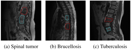
Fig. 7. MRI images of three types of lesions: brucellosis, tuberculosis, and tumor.
3.2. Implementation Details and Evaluation Metrics
To ensure the robustness and generalizability of the proposed model, we implemented a five-fold cross-validation strategy. The experimental procedure is delineated into the following three critical stages:
Step 1: Data Partitioning. The original dataset \(S\) was randomly partitioned into five mutually exclusive subsets \(\{S_{1},S_{2},S_{3},S_{4},S_{5}\}\).
Step 2: Five-Fold Cross-Validation Protocol (\(i=1,\dots,5\)). For the \(i\)-th iteration, the training set and the test set are defined respectively as \(\mathit{Train}_{i}\) and \(\mathit{Test}_{i}\). Classification performance was rigorously evaluated on the independent test set \(\mathit{Test}_{i}\).
Step 3: Final Performance Synthesis. The overall diagnostic efficacy was estimated by averaging the metrics across all five folds. We utilized four primary metrics: Accuracy, Precision (\(P\)), Recall (\(R\)), and F1-score. Given the clinical imperative in oncology to minimize false negatives, priority was given to Recall (Sensitivity), with the classification confidence threshold set to 0.90 to ensure high diagnostic sensitivity.
In the context of identifying spinal tumors, the performance metrics are defined as follows:
-
・
True Positives (TP): The number of instances that are actually spinal tumors and are correctly predicted as such.
-
・
False Positives (FP): The number of instances that are actually non-tumors but are incorrectly predicted as spinal tumors.
-
・
False Negatives (FN): The number of instances that are actually spinal tumors but are incorrectly predicted as non-tumors.
-
・
True Negatives (TN): The number of instances that are actually non-tumors and are correctly predicted as such.
These metrics are calculated in the same manner for the diagnosis of brucellosis and tuberculosis.
3.3. Experimental Procedure and Analysis
The experiments were conducted on an Ubuntu 22 platform equipped with an NVIDIA Tesla V100 GPU. During the training process, the input image size was set to \({224 \times 224}\), and the batch size was set to 128. We utilized the AdamW optimizer with an initial learning rate of 0.001. The model was trained for a maximum of 100 epochs, incorporating an early stopping strategy to prevent overfitting. If the loss failed to decrease by more than \(10^{-11}\) for 20 consecutive epochs, training was terminated prematurely, and the weights yielding the best performance were preserved. As presented in Table 3, the ablation study on the modified backbone model demonstrates its enhanced performance. The improved model achieved both an accuracy and a precision of 93.7% for spinal lesion identification. Compared to the original model, this significant improvement is primarily attributed to the advantages of the BiFPN in target recognition. However, spinal lesions in MRI scans often exhibit considerable morphological variation, and their positional information can be obscured by background noise. To address this, standard convolution kernels in certain feature layers of the backbone were replaced with DCN, which is more effective at capturing features of small targets. The integration of the DCN module into the BiFPN architecture resulted in a 0.8% increase in precision and a 0.6% increase in recall compared to the original model. This confirms that the combination of bidirectional multi-scale feature fusion (from BiFPN) and deformable convolution (from DCN) leads to more effective feature extraction.
| Model components | Performance metrics | ||||||||||
| Baseline |
Multi-scale feature fusion |
BiFPN | DCN | Accuracy [%] | Precision [%] | Recall [%] | F1-score [%] | ||||
| ✓ | 92.3\(\pm\)0.97 | 92.9\(\pm\)1.12 | 87.2\(\pm\)0.92 | 89.9\(\pm\)0.7 | |||||||
| ✓ | ✓ | 92.4\(\pm\)1.05 | 92.9\(\pm\)0.87 | 87.5\(\pm\)1.19 | 90.1\(\pm\)0.8 | ||||||
| ✓ | ✓ | ✓ | 92.9\(\pm\)0.73 | 92.4\(\pm\)0.58 | 87.6\(\pm\)0.78 | 89.9\(\pm\)0.5 | |||||
| ✓ | ✓ | 93.1\(\pm\)0.76 | 93.3\(\pm\)1.12 | 87.6\(\pm\)1.60 | 90.4\(\pm\)1.0 | ||||||
| ✓ | ✓ | ✓ | ✓ | 93.7\(\pm\)0.85 | 93.7\(\pm\)0.71 | 87.8\(\pm\)0.52 | 90.7\(\pm\)0.6 | ||||
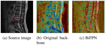
Fig. 8. Activation map from the enhanced backbone network.
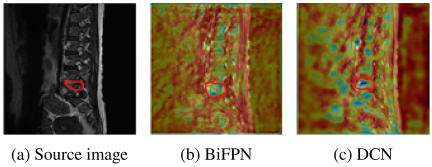
Fig. 9. Feature heatmap with the integration of DCN.
Given the requirements for heatmap visualization, the M2 layer was chosen because it benefits from multi-stage feature fusion. This allows it to capture sufficient semantic information while maintaining a relatively high spatial resolution. Fig. 8 visualizes the enhancement in feature extraction via heatmaps, where the red-annotated region indicates the lesion. The visualization demonstrates that whereas the original backbone network produced diffuse activations across both the lesion and other spinal regions, the feature map refined by BiFPN exhibits highly localized and intense activation specifically on the lesion, rendering it markedly more conspicuous.
Figure 9 demonstrates the effect of introducing DCN on feature representation, with the lesion highlighted in red. The visualization confirms that DCN markedly intensifies the features specific to the lesion, leading to a more focused and discriminative activation map.
The results of the ablation experiments conducted on the multi-attention mechanisms are detailed in Table 4. Following these modifications, the proposed model demonstrates a recognition accuracy of 93.8% and a precision of 93.9% for the task of spinal lesion identification. A comparative analysis reveals that integrating the self-attention (TAC) module into the final feature map yields a substantial 1.1 percentage point increase in accuracy over the baseline. This enhancement is attributed to the module’s capacity for capturing global contextual information. Moreover, the incorporation of the Soft Attention (SAC) module, which leverages enriched positional and feature information, elevated the model’s precision by 1.0% and its recall by 1.1% when benchmarked against the original architecture.
The results of the ablation study on the loss function are presented in Table 5. To address the class imbalance problem, we first introduced the BCE loss. By assigning different weights to each class, BCE effectively improved the model’s recognition accuracy. We further evaluated Focal Loss, which not only considers the importance of different samples but also introduces a modulating factor to differentiate between easy and hard examples. The model incorporating Focal Loss achieved the best performance, improving the recall by 1.3% compared to the baseline model.
| Model components | Performance metrics | |||||||||
| Baseline | TAC | SAC | Accuracy [%] | Precision [%] | Recall [%] | F1-score [%] | ||||
| ✓ | 92.3\(\pm\)0.97 | 92.9\(\pm\)1.12 | 87.2\(\pm\)0.92 | 89.9\(\pm\)0.7 | ||||||
| ✓ | ✓ | 93.4\(\pm\)0.34 | 92.4\(\pm\)0.49 | 88.1\(\pm\)0.38 | 90.2\(\pm\)0.3 | |||||
| ✓ | ✓ | 93.0\(\pm\)0.57 | 93.7\(\pm\)0.85 | 88.1\(\pm\)0.71 | 90.8\(\pm\)0.5 | |||||
| ✓ | ✓ | ✓ | 93.8\(\pm\)0.61 | 93.9\(\pm\)0.40 | 88.3\(\pm\)0.47 | 91.0\(\pm\)0.4 | ||||
| Model configuration | Performance metrics | |||||||||
| Baseline (CE) | Balanced CE | Focal loss | Accuracy [%] | Precision [%] | Recall [%] | F1-score [%] | ||||
| ✓ | 92.3\(\pm\)0.97 | 92.9\(\pm\)1.12 | 87.2\(\pm\)0.92 | 89.9\(\pm\)0.7 | ||||||
| ✓ | ✓ | 93.4\(\pm\)1.03 | 93.0\(\pm\)1.80 | 87.2\(\pm\)1.45 | 90.0\(\pm\)1.0 | |||||
| ✓ | ✓ | 93.8\(\pm\)0.71 | 93.0\(\pm\)1.10 | 88.5\(\pm\)0.56 | 90.7\(\pm\)0.6 | |||||
To verify the contribution of each component, an ablation study was conducted, as shown in Table 6. Building upon Baseline Model A, Model B introduced a backbone network featuring multi-scale fusion and bidirectional enhancement. Model C further incorporated DCN into Model B to form an improved backbone, achieving an accuracy of \(93.7{\pm}0.85\)% and an F1-score of \(90.7{\pm}0.6\)%. This improvement indicates that DCN and BiFPN are complementary, significantly enhancing the model’s capability to capture complex features. Meanwhile, Model D integrated a multi-attention mechanism, yielding an accuracy of \(93.8{\pm}0.61\)% and an F1-score of \(91.0{\pm}0.4\)%, which demonstrates the advantage of multi-attention in extracting discriminative features for pathological lesions. Model E introduced an optimized loss function to further refine recognition performance. Finally, the proposed model (Model F) achieved \(96.6{\pm}0.56\)% accuracy, \(94.2{\pm}0.40\)% precision, \(90.8{\pm}0.48\)% recall, and \(92.5{\pm}0.4\)% F1-score. Compared to the baseline, the accuracy and F1-score increased by 4.3% and 2.6%, respectively. Model F outperformed all single-module optimizations, demonstrating a clear synergistic effect among the components. The qualitative results are visualized in Fig. 10. As depicted, the proposed model accurately detects lesion regions and robustly identifies spinal tumors, brucellosis, and tuberculosis, even in the presence of noise and despite significant variations in lesion location, structure, and size.
| Model configuration | Performance metrics | ||||||||
| ID | Description | Accuracy [%] | Precision [%] | Recall [%] | F1-score [%] | ||||
| A | Baseline model | 92.3\(\pm\)0.97 | 92.9\(\pm\)1.12 | 87.2\(\pm\)0.92 | 89.9\(\pm\)0.7 | ||||
| B | Baseline + BiFPN | 92.9\(\pm\)0.73 | 92.4\(\pm\)0.58 | 87.6\(\pm\)0.78 | 89.9\(\pm\)0.5 | ||||
| C | Baseline + BiFPN + DCN | 93.7\(\pm\)0.85 | 93.7\(\pm\)0.71 | 87.8\(\pm\)0.52 | 90.7\(\pm\)0.6 | ||||
| D | Baseline + Multiple Attention Mechanism | 93.8\(\pm\)0.61 | 93.9\(\pm\)0.40 | 88.3\(\pm\)0.47 | 91.0\(\pm\)0.4 | ||||
| E | Baseline + Focal Loss | 93.8\(\pm\)0.71 | 93.0\(\pm\)1.10 | 88.5\(\pm\)0.56 | 90.7\(\pm\)0.6 | ||||
| F | Proposed model (all enhancements) | 96.6\(\pm\)0.56 | 94.2\(\pm\)0.40 | 90.8\(\pm\)0.48 | 92.5\(\pm\)0.4 | ||||
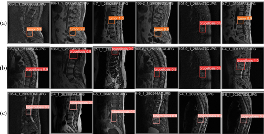
Fig. 10. Visualization of the model’s classification results. The input images are correctly identified as (a) tumor, (b) brucellosis, and (c) tuberculosis.
| Predicted label | |||
| True label | Spinal tumor | Brucellosis | Tuberculosis |
| Spinal tumor | 368 | 0 | 30 |
| Brucellosis | 53 | 337 | 10 |
| Tuberculosis | 17 | 0 | 383 |
Table 7 presents the confusion matrix of our proposed model on the test dataset. As shown in the table, the high values along the main diagonal significantly outweigh the off-diagonal elements, indicating that the model correctly classified the majority of lesions. Specifically, for the tumor class, 368 samples were accurately identified, with only 2 being missed (false negatives). For tuberculosis, 383 samples were correctly classified, while 17 were misclassified. The model’s performance on brucellosis, however, was more challenging; it was frequently misclassified as tumor. This difficulty is largely attributed to two factors. First, the rarity of brucellosis leads to a severe class imbalance in the dataset, causing the model to be biased towards the features of more common diseases. Second, this challenge mirrors the diagnostic difficulties in clinical practice, where the imaging manifestations of brucellosis are highly similar to those of spinal tumors, often leading to misdiagnosis. In our future work, we plan to employ methods such as adversarial training to reduce the misclassification rate for the rare brucellosis class.
To further evaluate the model’s generalizability, a subgroup analysis stratified by (1) lesion size (\({<}10\) mm, 10–30 mm, and \({>}30\) mm) and (2) vertebral level (cervical, thoracic, and lumbar/sacral) was performed. Specifically, lesion size was defined by the maximal axis measured on MRI, while vertebral levels were categorized according to standard anatomical criteria. The variable \(N\) denotes the number of images in each subgroup, drawn from a total test set of \(N=1200\). These results, including per-subgroup Accuracy, Precision, Recall, and F1-score, are detailed in Table 8. The findings demonstrate that the model’s performance remains consistent across all subgroups, further validating the robustness of the proposed method.
| ID | Subgroup configuration | N (test) | Accuracy [%] | Precision [%] | Recall [%] | F1-score [%] |
| By lesion size | ||||||
| 1 | Lesion size \(<\) 10 mm | 543 | \(92.16{\pm}0.58\) | \(90.76{\pm}0.96\) | \(89.82{\pm}0.45\) | \(90.3{\pm}0.5\) |
| 2 | Lesion size 10–30 mm | 522 | \(97.23{\pm}1.28\) | \(96.36{\pm}2.04\) | \(90.21{\pm}1.02\) | \(93.2{\pm}1.1\) |
| 3 | Lesion size \(>\) 30 mm | 135 | \(99.40{\pm}0.34\) | \(95.18{\pm}1.89\) | \(92.76{\pm}1.72\) | \(94.0{\pm}1.3\) |
| By vertebral level | ||||||
| 4 | Cervical (C1–C7) | 201 | \(96.99{\pm}0.29\) | \(94.20{\pm}0.32\) | \(90.76{\pm}1.98\) | \(92.4{\pm}1.1\) |
| 5 | Thoracic (T1–T12) | 567 | \(96.58{\pm}0.20\) | \(94.25{\pm}0.25\) | \(90.50{\pm}1.56\) | \(92.3{\pm}0.9\) |
| 6 | Lumbar/sacral | 432 | \(96.34{\pm}0.24\) | \(94.96{\pm}1.05\) | \(90.98{\pm}0.63\) | \(92.9{\pm}0.6\) |
| Model | Accuracy [%] | Precision [%] | Recall [%] | F1-score [%] |
| VGG-19 20 | 92.3\(\pm\)1.6 | 75.6\(\pm\)1.9 | 67.3\(\pm\)1.7 | 71.2\(\pm\)1.2 |
| DenseNet 21 | 89.0\(\pm\)1.3 | 80.1\(\pm\)1.2 | 77.3\(\pm\)1.1 | 78.7\(\pm\)0.8 |
| Faster R-CNN 22 | 80.2\(\pm\)1.4 | 73.0\(\pm\)1.7 | 63.2\(\pm\)1.5 | 67.8\(\pm\)1.1 |
| Deformable_DETR 23 | 80.8\(\pm\)0.9 | 68.6\(\pm\)1.0 | 67.4\(\pm\)0.9 | 68.0\(\pm\)0.7 |
| FPN | 92.3\(\pm\)0.5 | 75.6\(\pm\)0.6 | 67.3\(\pm\)0.9 | 71.2\(\pm\)0.5 |
| YOLOv8 24 | 89.0\(\pm\)1.2 | 80.1\(\pm\)1.3 | 89.0\(\pm\)1.2 | 84.3\(\pm\)0.9 |
| PSPNet 25 | 83.7\(\pm\)0.8 | 81.6\(\pm\)0.7 | 88.1\(\pm\)0.8 | 84.7\(\pm\)0.5 |
| DeepLabV3 26 | 85.8\(\pm\)1.1 | 89.4\(\pm\)1.1 | 85.4\(\pm\)1.3 | 87.4\(\pm\)0.8 |
| U-Net++ 27 | 92.6\(\pm\)0.9 | 88.7\(\pm\)0.8 | 87.9\(\pm\)1.0 | 88.3\(\pm\)0.6 |
| SpineNet 28 | 84.2\(\pm\)0.6 | 84.6\(\pm\)0.7 | 84.2\(\pm\)1.0 | 84.4\(\pm\)0.6 |
| CornerNet 29 | 88.7\(\pm\)0.4 | 95.2\(\pm\)0.4 | 88.9\(\pm\)0.3 | 91.9\(\pm\)0.2 |
| RT-DETR 30 | 80.7\(\pm\)0.8 | 66.0\(\pm\)0.6 | 62.3\(\pm\)0.7 | 64.1\(\pm\)0.5 |
| Our model | 96.6\(\pm\)0.56 | 94.2\(\pm\)0.40 | 90.8\(\pm\)0.48 | 92.5\(\pm\)0.4 |
3.4. Comparison with Other Models
The comparative results presented in Table 9 demonstrate the superiority of our proposed model over other methods. Specifically, on the given dataset, our model achieves significantly higher classification accuracies for the three diseases compared to the second-best model, U-Net++. While the precision of our model is slightly lower than that of CornerNet, it achieves a superior F1-score. This indicates a more effective balance between precision and recall, suggesting better overall performance. These results affirm the advanced lesion identification capabilities of our model. This enhanced performance is attributed to its architecture, which leverages a bidirectional feature fusion network and deformable convolutions to extract more robust feature representations, while multiple attention mechanisms optimize the utilization of this information. Consequently, our model achieves higher accuracy in identifying spinal lesions from MRI images.
3.5. Comparison with Other Classifications
To further validate the identification performance of our proposed model, we conducted a comparative study against several traditional machine-learning classifiers. These classifiers included KNN, SVM, naïve Bayes, and decision tree. The performance comparison is summarized in Table 10. The results clearly indicate that our model achieved an accuracy of 96.6%, significantly outperforming all other classifiers. The Decision Tree classifier delivered the second-best performance with an accuracy of 92.1%, whereas the KNN classifier yielded the lowest accuracy at only 87.6%. These findings demonstrate that our model possesses superior robustness and classification capability for spinal tumor identification compared to these conventional machine learning approaches.
| Classifier | Accuracy [%] |
| Deep features + KNN | \(87.6{\pm}1.80\) |
| Deep features + Naïve Bayes | \(88.2{\pm}1.70\) |
| Deep features + SVM | \(88.7{\pm}1.50\) |
| Deep features + Decision Tree | \(92.1{\pm}0.90\) |
| Our model | \(\textbf{96.6}{\boldsymbol{\pm}}\textbf{0.56}\) |
4. Conclusion
To address the challenges of qualitatively analyzing spinal lesions from MRI images, particularly the difficulty in distinguishing spinal tumors from infectious diseases like tuberculosis and rare conditions such as brucellosis, we propose a novel identification model. The model’s architecture improves upon a standard backbone by incorporating a BiFPN for more thorough feature fusion. Furthermore, we replaced select standard convolutions with deformable convolutions to enhance the feature representation capabilities of the backbone. Self-attention and flexible attention mechanisms were also integrated to capture crucial feature dependencies across different channels. Experimental results demonstrate the advancement and effectiveness of our model, indicating its potential to enhance clinicians’ diagnostic accuracy. However, we also observed that while the proposed method achieves superior identification performance, it does not entirely eliminate misdetections and missed detections, especially for the rare brucellosis cases. This limitation is primarily attributed to the scarcity of brucellosis samples and the model’s insufficient sensitivity to low-contrast features. To strengthen the representation of small lesion features, future network reconstruction will prioritize weighted fusion strategies. Meanwhile, we plan to introduce a dynamic annealing strategy into the balanced cross-entropy method. This involves the dynamic adjustment of key parameters, including loss weights, data augmentation factors, and learning rates, based on real-time training and validation metrics. It should be noted that treating slices from the same patient as independent samples in the test set may lead to an overestimation of performance. In future work, we will increase the sample size of independent subjects and adopt subject-level stratified cross-validation to further improve the robustness and generalizability of the model.
Acknowledgments
This research was funded by the Artificial intelligence-based assisted diagnosis of bone tumors and lesions in surgery, “Integrative Intelligence and Interdisciplinary, Medicine-Engineering” (LH-JSRZ-202203)
- [1] X. Chen, Y. Sun, J. Ju, and Y. Zheng, “Diagonistic and prognostic analysis of olfactory neuroblastoma,” J. Clin. Otorhinolaryngol. Head Neck Surg., Vol.35, No.3, pp. 224-228, 2021 (in Chinese). https://doi.org/10.13201/j.issn.2096-7993.2021.03.007
- [2] P. Klimo, Jr. and M. H. Schmidt, “Surgical management of spinal metastases,” Oncologist, Vol.9, No.2, pp. 188-196, 2004. https://doi.org/10.1634/theoncologist.9-2-188
- [3] D. M. Sciubba et al., “Diagnosis and management of metastatic spine disease: A review,” J. Neurosurg. Spine, Vol.13, No.1, pp. 94-108, 2010. https://doi.org/10.3171/2010.3.SPINE09202
- [4] A. Hosny et al., “Deep learning for lung cancer prognostication: A retrospective multi-cohort radiomics study,” PLOS Med., Vol.15, No.11, Article No.e1002711, 2018. https://doi.org/10.1371/journal.pmed.1002711
- [5] S. Boriani, J. N. Weinstein, and R. Biagini, “Primary bone tumors of the spine: Terminology and surgical staging,” Spine, Vol.22, No.9, pp. 1036-1044, 1997. https://doi.org/10.1097/00007632-199705010-00020
- [6] A. Mesfin, M. H. El Dafrawy, A. Jain, H. Hassanzadeh, and K. M. Kebaish, “Total en bloc spondylectomy for primary and metastatic spine tumors,” Orthopedics, Vol.38, No.11, pp. e995-e1000, 2015. https://doi.org/10.3928/01477447-20151020-08
- [7] Y. Li and W. Ping, “Cancer metastasis detection with neural conditional random field,” arXiv:1806.07064, 2018. https://doi.org/10.48550/arXiv.1806.07064
- [8] Q. Shao, L. Gong, K. Ma, H. Liu, and Y. Zheng, “Attentive CT lesion detection using deep pyramid inference with Multi-Scale Booster,” Proc. 22nd Int. Conf. Med. Image Comput. Comput.-Assist. Interv. (MICCAI 2019), Part VI, pp. 301-309, 2019. https://doi.org/10.1007/978-3-030-32226-7_34
- [9] M. I. Sharif, M. A. Khan, M. Alhussein, K. Aurangzeb, and M. Raza, “A decision support system for multimodal brain tumor classification using deep learning,” Complex Intell. Syst., Vol.8, No.4, pp. 3007-3020, 2022. https://doi.org/10.1007/s40747-021-00321-0
- [10] J. Coburger et al., “Low-grade glioma surgery in intraoperative magnetic resonance imaging: Results of a multicenter retrospective assessment of the German Study Group for Intraoperative Magnetic Resonance Imaging,” Neurosurgery, Vol.78, No.6, pp. 775-786, 2016. https://doi.org/10.1227/NEU.0000000000001081
- [11] N. Lang et al., “Differentiation of spinal metastases originated from lung and other cancers using radiomics and deep learning based on DCE-MRI,” Magn. Reson. Imaging, Vol.64, pp. 4-12, 2019. https://doi.org/10.1016/j.mri.2019.02.013
- [12] V. Chianca et al., “Radiomic machine learning classifiers in spine bone tumors: A multi-software, multi-scanner study,” Eur. J. Radiol., Vol.137, Article No.109586, 2021. https://doi.org/10.1016/j.ejrad.2021.109586
- [13] J. O. B. Diniz, P. H. B. Diniz, T. L. A. Valente, A. C. Silva, and A. C. Paiva, “Spinal cord detection in planning CT for radiotherapy through adaptive template matching, IMSLIC and convolutional neural networks,” Comput. Methods Programs Biomed., Vol.170, pp. 53-67, 2019. https://doi.org/10.1016/j.cmpb.2019.01.005
- [14] Z. Li et al., “Computer-aided diagnosis of spinal tuberculosis from CT images based on deep learning with multimodal feature fusion,” Front. Microbiol., Vol.13, Article No.823324, 2022. https://doi.org/10.3389/fmicb.2022.823324
- [15] S. R. S. Arends et al., “Clinical utility of convolutional neural networks for treatment planning in radiotherapy for spinal metastases,” Phys. Imaging Radiat. Oncol., Vol.21, pp. 42-47, 2022. https://doi.org/10.1016/j.phro.2022.02.003
- [16] J. Olczak et al., “Artificial intelligence for analyzing orthopedic trauma radiographs,” Acta Orthop., Vol.88, No.6, pp. 581-586, 2017. https://doi.org/10.1080/17453674.2017.1344459
- [17] S. L. Goldenberg, G. Nir, and S. E. Salcudean, “A new era: Artificial intelligence and machine learning in prostate cancer,” Nat. Rev. Urol., Vol.16, No.7, pp. 391-403, 2019. https://doi.org/10.1038/s41585-019-0193-3
- [18] G. Ghiasi, T.-Y. Lin, and Q. V. Le, “NAS-FPN: Learning scalable feature pyramid architecture for object detection,” Proc. 2019 IEEE/CVF Conf. Comput. Vis. Pattern Recognit. (CVPR), pp. 7029-7038, 2019. https://doi.org/10.1109/CVPR.2019.00720
- [19] Y.-L. Tian, Y.-T. Wang, J.-G. Wang, X. Wang, and F.-Y. Wang, “Key problems and progress of vision Transformers: The state of the art and prospects,” Acta Autom. Sin., Vol.48, No.4, pp. 957-979, 2022 (in Chinese). https://doi.org/10.16383/j.aas.c220027
- [20] L. Wen, X. Li, X. Li, and L. Gao, “A new transfer learning based on VGG-19 network for fault diagnosis,” 2019 IEEE 23rd Int. Conf. Comput. Support. Coop. Work Des. (CSCWD), pp. 205-209, 2019. https://doi.org/10.1109/CSCWD.2019.8791884
- [21] Y. Zhu and S. Newsam, “DenseNet for dense flow,” 2017 IEEE Int. Conf. Image Process. (ICIP), pp. 790-794, 2017. https://doi.org/10.1109/ICIP.2017.8296389
- [22] M. Kang, X. Leng, Z. Lin, and K. Ji, “A modified faster R-CNN based on CFAR algorithm for SAR ship detection,” 2017 Int. Workshop Remote Sens. Intell. Process. (RSIP), 2017. https://doi.org/10.1109/RSIP.2017.7958815
- [23] J. Dai et al., “Deformable convolutional networks,” 2017 IEEE Int. Conf. Comput. Vis. (ICCV), pp. 764-773, 2017. https://doi.org/10.1109/ICCV.2017.89
- [24] G. Wang et al., “UAV-YOLOv8: A small-object-detection model based on improved YOLOv8 for UAV aerial photography scenarios,” Sensors, Vol.23, No.16, Article No.7190, 2023. https://doi.org/10.3390/s23167190
- [25] Y. Chen, J. Wang, Y. Zhang, Y. Liu, and J. Wang, “P2RNet: Fast maritime object detection from key points to region proposals in large-scale remote sensing images,” IEEE J. Sel. Top. Appl. Earth Obs. Remote Sens., Vol.17, pp. 9294-9308, 2024. https://doi.org/10.1109/JSTARS.2024.3392635
- [26] Y. Liu et al., “Image semantic segmentation approach based on DeepLabV3 plus network with an attention mechanism,” Eng. Appl. Artif. Intell., Vol.127, Part A, Article No.107260, 2024. https://doi.org/10.1016/j.engappai.2023.107260
- [27] Z. Zhou, M. M. R. Siddiquee, N. Tajbakhsh, and J. Liang, “UNet++: A nested U-Net architecture for medical image segmentation,” Proc. 4th Int. Workshop Deep Learn. Med. Image Anal. 8th Multimodal Learn. Clin. Decis. Support (DLMIA/ML-CDS 2018), pp. 3-11, 2018. https://doi.org/10.1007/978-3-030-00889-5_1
- [28] X. Du et al., “SpineNet: Learning scale-permuted backbone for recognition and localization,” 2020 IEEE/CVF Conf. Comput. Vis. Pattern Recognit. (CVPR), pp. 11589-11598, 2020. https://doi.org/10.1109/CVPR42600.2020.01161
- [29] H. Law and J. Deng, “CornerNet: Detecting objects as paired keypoints,” Int. J. Comput. Vis., Vol.128, No.3, pp. 642-656, 2020. https://doi.org/10.1007/s11263-019-01204-1
- [30] Y. Zhao et al., “DETRs beat YOLOs on real-time object detection,” 2024 IEEE/CVF Conf. Comput. Vis. Pattern Recognit. (CVPR), pp. 16965-16974, 2024. https://doi.org/10.1109/CVPR52733.2024.01605
This article is published under a Creative Commons Attribution-NoDerivatives 4.0 Internationa License.