
Research Paper:
Modeling Nonlinear and Time-Varying Price Discovery: A Novel Granger Causality Framework Based on Distributional Forecasting
Yanyun Yao*, Ziyuan Xie*,†, and Shangzhen Cai**
*College of Finance, Ningbo University of Finance & Economics
899 Xueyuan Road, Haishu District, Ningbo, Zhejiang 315175, China
†Corresponding author
**College of Artificial Intelligence, Ningbo University of Finance & Economics
899 Xueyuan Road, Haishu District, Ningbo, Zhejiang 315175, China

The price-leadership relationship between stock index futures and spot markets is crucial for assessing market efficiency and implementing risk management. Traditional Granger causality tests based on conditional methods cannot capture their nonlinear and time-varying characteristics. In this study, we innovatively construct a Granger causality testing framework based on distributional forecasting. By integrating nonlinear modeling, time-varying volatility estimation, and rolling-window distributional forecasting techniques, the framework identifies and characterizes the price-leadership mechanism from the perspective of out-of-sample forecast performance improvement. Monte Carlo simulations verify that the proposed test possesses desirable finite-sample properties. An empirical study of China’s CSI 300 stock index futures and spot markets reveals a significant bidirectional nonlinear leadership relationship with distinct time-varying features. Specifically, futures lead spot through linear information transmission with lags of three to four periods, whereas spot leads futures through a rapid one-period impact and continuous feedback with lags of three to four periods. The seemingly counter-intuitive three- to four-day lag is attributable to daily price limits, a retail-dominated investor structure, and arbitrage constraints. Cross-market transmission is dominated by linear spillovers, whereas nonlinear effects are primarily internalized within each market’s respective volatility structure. This study not only transcends the classical linear and static analysis paradigm but also provides new methodological support and a decision-making basis for optimizing dynamic hedging strategies and cross-market risk early warning.
1. Introduction
The price-leadership relationship between stock index futures and spot markets is fundamental for assessing market efficiency, designing hedging strategies, and informing regulatory policies. Understanding the direction and mechanism of information transmission between the two markets is essential for price discovery, risk management, and cross-market contagion prevention.
Previous studies typically rely on linear Granger causality tests within a conditional-mean framework, where vector autoregressions are used to determine whether one market’s past returns facilitate the prediction of other’s mean return 1,2,3. However, financial returns typically exhibit pronounced nonlinearity, time variations, and asymmetry, particularly during extreme events, regime shifts, or abrupt changes in investor sentiment. Linear models cannot capture such complex dynamics, thus casting doubt regarding the robustness of their conclusions 4,5,6.
Hence, nonlinear Granger causality tests, such as the nonparametric DP test 7 and LASSO-based approaches 8, have been developed. Meanwhile, quantile-based tests allow the analysis of asymmetric risk spillovers 9,10,11. Nevertheless, most of these methods focus on conditional expectations or specific quantiles and do not evaluate causality based on the entire conditional distribution of futures returns. Consequently, they may overlook volatility spillovers, tail dependence, and other higher-moment transmissions. Moreover, existing tests rely primarily on in-sample model fit (e.g., residual sum of squares comparisons) instead of on out-of-sample predictive performance, which is the essence of Granger’s original definition 12. A unified framework that combines nonlinear mean dynamics, time-varying volatility, and out-of-sample distributional forecast evaluation is yet to be established.
Hence, this study proposes a novel Granger causality testing framework based on distributional forecasting. This framework offers three key innovations:
-
(1)
From conditional mean to whole distribution: Instead of testing the mean or quantile predictability, we compare the entire out-of-sample conditional distribution of returns with and without another market’s information, thus adhering strictly to Granger’s 12 probabilistic definition.
-
(2)
Nonlinear mean + time-varying volatility: We integrate a nonlinear mean equation (LASSO with linear and quadratic lagged terms) with an EGARCH(1,1) volatility model to capture both the nonlinearity and leverage effects within a rolling-window forecasting scheme.
-
(3)
Strict distributional forecast evaluation: Causality is inferred by applying the HL test on probability integral transform (PIT) sequences 13 and the AG test on logarithmic scores 14, which requires the extended model to yield a correctly specified PIT sequence and significantly better log scores than the benchmark model.
For a methodological validation, we conduct Monte Carlo simulations to examine the finite-sample size and power of the proposed test. The simulation results confirm that the test maintains an empirical size close to the nominal level (0.05) and exhibits high power under linear and moderately strong nonlinear causality.
We empirically apply the framework to the CSI 300 stock index futures and spot markets from April 2010 to August 2022. Our analysis reveals a robust bidirectional nonlinear time-varying Granger causality. Specifically, futures lead spots through linear signals at lags 3–4, whereas spots lead futures through a rapid one-period impact and persistent feedback at lags 3–4. Transmission is dominated by cross-market linear spillovers, with nonlinear effects mainly internalized primarily within each market’s volatility structure. These findings provide guidance for dynamic hedging and cross-market risk monitoring.
The remainder of this paper is organized as follows: Section 2 reviews the relevant literature. Section 3 describes the methodology, including the distributional forecasting causality framework. Section 4 presents the Monte Carlo simulations performed to validate the finite-sample properties of the proposed test. Section 5 reports the empirical results, including the data description and findings from the CSI 300 futures and spot markets. Finally, Section 6 concludes the paper and discusses future research directions.
2. Literature Review
The price-discovery mechanism between stock index futures and spot markets is central to understanding market efficiency and risk transmission. Previous studies primarily assume linear and static relationships; however, real-world information transmission is typically nonlinear, asymmetric, and time varying, as it evolves with market conditions, policy shocks, and investor structures 15.
2.1. Nonlinear and Time-Varying Characteristics of Price Discovery
Early studies reported conflicting findings, such as futures dominance 1, spot dominance 2, and bidirectional leadership 3. More recent evidence suggests that leadership relationships are state dependent and time varying. For instance, Zhao et al. 4 observed heterogeneous lead-lag patterns between CSI 300 futures and spots in bull vs. bear markets; Li et al. 5 documented that during the 2015 Chinese stock market crash, the spot market temporarily dominated price discovery; and Ghedira and Nakhli 6 showed that causality between stock markets and oil prices changed across crisis phases. Additionally, non-linear linkages were detected in China’s multilevel capital markets 16 and interprovincial economic growth 17. These findings highlight the fact that disregarding nonlinearity and time variation may bias the inference of cross-market information flows.
2.2. Methodological Evolution of Granger Causality Tests
Granger 12 defined causality based on predictive ability: \(X\) Granger causes \(Y\) if past \(X\) helps predict \(Y\). Early tests operated within a linear conditional-mean framework (VAR models). To capture nonlinear dynamics, nonparametric tests (e.g., the DP test 7) and semiparametric approaches (e.g., LASSO-based tests 8) have been developed. Quantile causality tests allow one to further examine asymmetric risk spillovers 9,10,11. Despite these advances, most methods focus on conditional expectations or specific quantiles instead of on the entire conditional distribution of futures returns—the essence of Granger’s original definition. Moreover, they typically rely on in-sample fit comparisons instead of on out-of-sample predictive performance.
2.3. Limitations of Existing Studies and Contributions of Present Study
Three major discrepancies persist:
-
(1)
Prediction vs. explanation: Most tests assess in-sample fit, not out-of-sample distributional forecast improvement, thereby limiting their practical value for real-time risk management.
-
(2)
Nonconsideration of whole distribution: Quantile causality does not evaluate the full conditional distribution, thus rendering it impossible to capture volatility spillovers and tail-risk transmission.
-
(3)
Model integration: Few studies combine nonlinear mean dynamics with time-varying volatility in a rolling forecast framework.
Hence, this study proposes a distributional forecasting-based Granger causality test that integrates LASSO nonlinear mean equations, EGARCH volatility, and rigorous out-of-sample evaluation via PIT-based HL tests and logarithmic-score AG tests. Monte Carlo simulations validate its finite-sample properties, while an empirical application to CSI 300 futures and spot markets demonstrates its usefulness.
3. Models and Methods
3.1. Basic Definition of Granger Causality
Granger causality is defined based on predictive ability 12. Let \(I_{t-1}\) denote all available information up to time \(t-1\). In a bivariate setting, \(I_{t-1}\) contains the histories of \(X_t\) and \(Y_t\). From the perspective of conditional distribution, \(X\) does not Granger-cause \(Y\) if
In other words, including past information on \(X\) does not change the conditional distribution of \(Y_t\). Eq. (1) is the original definition; however, early studies typically simplify it to a conditional-mean comparison:
This simplification results in widely used linear and nonlinear tests based on conditional expectations, but fails to capture higher-moment dynamics, such as volatility spillovers and tail risks.
3.2. Conventional Test Methods and Their Limitations
3.2.1. Linear Granger Causality Test
Under framework (2), linear causality is typically tested via VAR. For two stationary series \(X_t\) and \(Y_t\), the null hypothesis that \(X\) does not Granger-cause \(Y\) is tested based on an \(F\)-statistic comparing restricted and unrestricted VAR models 1,2,3. Although simple and intuitive, linear tests cannot capture non-linear dependencies.
3.2.2. Nonlinear Granger Causality Tests
Nonparametric and semiparametric tests were conducted to capture nonlinearities. The DP test 7 uses kernel density estimation to test the conditional independence in Eq. (1) directly, thereby overcoming the over-rejection issue of earlier methods. The LASSO-based test 8 approximates an unknown function via a Taylor expansion and uses LASSO for variable selection, thus enabling the identification of specific nonlinear patterns (e.g., quadratic terms). Quantile causality tests 9,10,11 examine the predictability at specific quantiles and reveal asymmetric risk spillovers.
3.2.3. Tests Limitations of Existing Methods
Despite these advances, classical tests exhibit several limitations when applied to price discovery in futures and spot markets:
-
(1)
Focus on conditional moments: Most tests compare conditional expectations or specific quantiles while disregarding the entire distribution. Consequently, volatility spillovers and tail dependencies are overlooked.
-
(2)
In-sample fit vs. out-of-sample prediction: They rely on in-sample goodness-of-fit (e.g., RSS comparisons), which is not equivalent to out-of-sample predictive ability-the essence of Granger causality 12.
-
(3)
Non-integration with time-varying volatility: Nonlinear mean equations are commonly estimated separately from volatility dynamics, thus yielding incomplete conditional distribution forecasts.
-
(4)
Implicit stability assumption: Causality is assumed to be constant over time, whereas financial markets undergo structural changes.
3.3. Proposed Framework: Nonlinear Time-Varying Causality Test Based on Distributional Forecasting
3.3.1. Overall Logic and Rolling Forecast Mechanism
We return to Granger’s original definition 12 and compare the entire conditional distribution of futures returns with and without another market’s information. A rolling-window scheme is used to account for time variation. For each window, we estimate the following two models:
-
(1)
Benchmark model: Uses only own-market lags;
-
(2)
Extended model: Incorporates the lags (linear and quadratic) of another market.
One-step-ahead distribution forecasts are generated, and the out-of-sample sequences of PITs and logarithmic scores are evaluated.
3.3.2. Nonlinear Mean Equation: LASSO Variable Selection
Let \(Y_t\) be the return series (spot \(S_t\) or futures \(F_t\)). The conditional mean \(\mu_{t} = E(Y_{t}\mid I_{t-1})\) is modeled as a function of lagged linear and quadratic terms (up to lag \(p\) order). To avoid overfitting and identify relevant predictors, we apply LASSO to each rolling window as follows:
3.3.3. Time-Varying Volatility: EGARCH(1,1) and Skewed-\(t\) Distribution
To capture volatility clustering and asymmetry (the leverage effect), we use EGARCH(1,1) for the conditional variance as follows:
Stock-market volatility typically exhibits clustering, which justifies the use of GARCH-type models. However, when the actual data lack asymmetric effects, \(\gamma\) is insignificant. Consequently, in the Monte Carlo simulations presented in Section 4, the volatility process is specified as a GARCH model instead of an EGARCH model.
3.3.4. Distributional Forecast Evaluation: HL and AG Tests
After obtaining one-step-ahead forecast distributions from the benchmark and extended models over all the rolling windows, we apply two evaluation criteria:
-
(1)
PIT and HL test
For each forecast cumulative distribution function \(F_{t\mid t-1}\), we compute
\begin{equation} \mathit{PIT}_{t} = F_{t\mid t-1}\left(y_{t}\right). \label{eq:5} \tag{5} \end{equation}If the forecast distribution is correctly specified, then \(\mathit{PIT}_t\) should be i.i.d. uniform in \([0,1]\). The HL test 13 provides a nonparametric omnibus test for this property. A nonsignificant HL statistic indicates that the forecast distribution is well specified.
-
(2)
Logarithmic score and AG test
The logarithmic score is expressed as
\begin{equation} \mathit{LS}_{t} = -\ln f_{t\mid t-1}\left(y_t\right), \label{eq:6} \tag{6} \end{equation}where \(f\) denotes the forecast density. A lower score indicates better predictive accuracy. For the two competing models, we define
\begin{equation} d_{t} = \mathit{LS}_{t}^{\,(\mathit{bench})} - \mathit{LS}_t^{\,(\mathit{ext})}. \label{eq:7} \tag{7} \end{equation}
The AG test 14 verifies whether \(H_{0}\colon E(d_{t})=0\) (equal predictive accuracy). A significantly positive mean of \(d_{t}\) (the AG test rejects the null hypothesis) indicates that the extended model outperforms the benchmark.
Causality criterion: The extended model is said to Granger-cause \(Y\) (in the distributional forecasting sense) if (i) its HL test is insignificant (the model is correctly specified) and (ii) the AG test is significant with \(\bar{d}_t>0\) (better predictive accuracy).
3.3.5. Remark on Multi-Step-Ahead Forecasting
Granger’s original definition is based on a one-step-ahead prediction 12. Multistep forecasts from EGARCH models tend to accumulate nonlinear errors, which can distort inferences. Therefore, this study focused on one-step-ahead forecasts.
4. Monte Carlo Simulation
Monte Carlo simulations were conducted to evaluate the finite-sample performance of the distributional forecasting Granger causality test proposed in Section 3.3, including the empirical size and power. To simplify the data-generating process (DGP) and focus on detecting causality, we adopt the standard GARCH(1,1) model to accommodate the volatility of the DGP. Notably, the proposed test is robust to symmetric volatility (as confirmed by the simulation results). A more complex EGARCH specification with leverage effects is reserved for an empirical application, which is justified by the data.
4.1. Simulation Design
Three DGPs are specified:
DGP1 (no causality, \(\boldsymbol{\mathrm{H}}_{\boldsymbol{0}}\)): \(X_t\) and \(Y_t\) are independent, with each adhering to a GARCH(1,1) process:
DGP2 (linear causality): A linear term, \(X_{t-1}\), is added to the mean equation of \(Y_t\) as follows:
DGP3 (nonlinear causality): The squared term \(X_{t-1}\) is added to the mean equation of \(Y_t\) as follows:
The sample sizes were set to \({T=1000}\) and \({T=2000}\), with a fixed rolling window length of 500. Consequently, the number of out-of-sample forecasts was 500 for \({T=1000}\) and 1500 for \({T=2000}\). For each DGP and sample size, 1000 replications were performed. In each replication, the following distributional forecasting causality-testing procedure was performed:
-
(1)
A rolling LASSO-EGARCH estimation was applied to the simulated \(Y_t\) series. The mean equation included lags up to order four (including the first-order and quadratic terms of \(Y_t\) totaling 14 variables). One-step-ahead distribution forecasts \(F_{t+1}\) were generated.
-
(2)
The first- and second-order lagged terms of both \(X\) and \(Y\) up to order four (44 variables in total) were added to the mean equation. A rolling LASSO–EGARCH estimation was performed to generate the one-step-ahead distribution forecast \(G_{t+1}\).
-
(3)
PIT sequences of \(F_{t+1}\) and \(G_{t+1}\) were obtained. The HL test statistics \(W\) were computed. The proportion \(p_{1}\) of times that the \(W\) statistic for \(G_{t+1}\) was smaller than that for \(F_{t+1}\) (i.e., \(G_{t+1}\) outperformed \(F_{t+1}\)) was recorded.
-
(4)
The AG test was applied to \(F_{t+1}\) and \(G_{t+1}\), and the proportion \(p_{2}\) of times that \(G_{t+1}\) outperformed \(F_{t+1}\) was recorded.
For DGP1 (no causality), \(p_{1}\) and \(p_{2}\) represent the rejection rates of \(\mathrm{H}_{0}\), i.e., the empirical size. For DGP2 or DGP3 (causality present), \(p_{1}\) and \(p_{2}\) represent the correct rejection rates of \(\mathrm{H}_{0}\), i.e., the empirical power.
4.2. Simulation Results
The simulation results are summarized in Table 1.
| DGP | Sample size | Out-of-sample forecasts | Number of rejections | Size (\(p_1\)) | Power (\(p_2\)) |
| DGP1 | \(T=1000\) | 500 | 26 | 0.052 | – |
| DGP1 | \(T=2000\) | 1500 | 73 | 0.049 | – |
| DGP2 | \(T=1000\) | 500 | 434 | – | 0.868 |
| DGP2 | \(T=2000\) | 1500 | 1434 | – | 0.956 |
| DGP3 | \(T=1000\) | 500 | 416 | – | 0.832 |
| DGP3 | \(T=2000\) | 1500 | 1411 | – | 0.941 |
Here, size denotes the probability of committing a Type I error. Based on Table 1, under the no-causality DGP, the empirical size was 0.052 for \({T=1000}\) and 0.049 for \({T=2000}\), both of which are almost identical to the nominal significance level of 0.05. This indicates that the proposed test is not affected by over-rejection and that Type I error is well controlled.
Power denotes the probability of not committing a Type II error. Table 1 shows that under linear causality, the power was 0.868 for \({T=1000}\) and increased to 0.956 for \({T=2000}\). This demonstrates the high ability of the test to detect linear causality and that its performance improves as the sample size increases. Under nonlinear causality, the power was slightly lower than that in the linear case but remained at a high level, which is expected because nonlinear effects are generally more difficult to detect.
The simulation results verified that the proposed distributional forecasting Granger causality test possessed desirable statistical properties under finite samples: the empirical size was close to the nominal level and the power was high.
5. Empirical Study
5.1. Data
This study investigates the price-leadership relationship between stock index futures and spot markets using China’s CSI 300 index futures launched on April 16, 2010. The underlying CSI 300 Index includes 300 large-cap, liquid stocks from the Shanghai and Shenzhen exchanges, thus rendering it a representative sample for analyzing China’s futures-spot linkage.
To avoid nonsynchronous trading noise (spot market: 9:30–11:30 and 13:00–15:00; futures market: 9:15–11:30 and 13:00–15:15), daily closing prices were used. The spot price is the CSI 300 Index closing price; the futures price is the daily settlement price of the front-month continuous contract. The sample period is from April 16, 2010 to August 2, 2022. After removing nontrading days, 2989 valid daily price observations were obtained.
Logarithmic percentage returns are computed as
The sample yielded 2988 return pairs. The Pearson correlation coefficient between \(S_t\) and \(F_t\) was 0.930, thus indicating strong co-movement. Augmented Dickey–Fuller tests rejected the unit root hypothesis at the 1% level for both series, thus confirming stationarity.
5.2. Causality Tests Based on Explanatory Perspective
5.2.1. Testing Approach
Following the standard Granger causality logic, we compared two sets of models (Table 2). Model 1 (S\(\sim\)S) uses only spot lags and Model 2 (S\(\sim\)S+F) incorporates futures lags.
Similarly, Model 3 (F\(\sim\)F) uses only futures lags and Model 4 (F\(\sim\)F+S) incorporates spot lags.
| Model | Notation | Meaning | Causality-testing approach |
| Model 1 | S\(\sim\)S | Spot return model; explanatory information only includes spot lags | Compare Models 1 and 2 to verify if futures is a Granger-cause of spots |
| Model 2 | S\(\sim\)S+F | Spot return model; explanatory information includes futures and spot lags | |
| Model 3 | F\(\sim\)F | Futures return model; explanatory information only includes futures lags | Compare Models 3 and 4 to verify if spot is a Granger-cause of futures |
| Model 4 | F\(\sim\)F+S | Futures return model; explanatory information includes futures and spot lags | |
| Note: F denotes futures returns, and S denotes spot returns. | |||
5.2.2. Linear Causality Test
We estimate a VAR(4) model (optimal lag by the SC criterion) for the full sample. Linear Granger causality results (Table 3) show that at the 5% level, we cannot reject “Futures does not Granger-cause spot” (\({p=0.0516}\)); however, we clearly rejected “Spot does not Granger-cause futures” (\({p=0.0302}\)). Thus, from a linear-mean perspective, spots lead futures, whereas futures’ lead over spots is only marginally significant.
| Linear-causality test | Nonlinear DP-causality test | |||
| Null hypothesis | \(F\)-statistic | \(p\)-value | DP Statistic | \(p\)-value |
| F is not a Granger-cause of S | 8.9275 | 0.0516 | 3.184 | 0.00073 |
| S is not a Granger-cause of F | 12.847 | 0.0302 | 1.907 | 0.02828 |
5.2.3. Nonlinear-Causality Test
-
(1)
The BDS test on VAR(4) residuals strongly rejects the i.i.d. (\(p<0.01\)), thus confirming a nonlinear structure.
- (2)
-
(3)
The LASSO-based test 8 (Taylor expansion to quadratic terms, Table 4) shows that adding information pertaining to other markets substantially improves the model fit (RSS decreases, LM statistics significant at 1%). The LASSO selects many quadratic terms (e.g., \(S_{t-1}^2\)), thus confirming nonlinearity.(1)
| Model | Minimum Cp value | Number of significant variables | RSS | \(R^2\) | LM statistic | \(p\)-value |
| S\(\sim\)S | 3.071802 | 1 | 6130.163 | 0.006 | 6.638 | 0 |
| S\(\sim\)S+F | 35.15957 | 38 | 5741.178 | 0.0687 | ||
| F\(\sim\)F | 11.68216 | 12 | 7317.037 | 0.0213 | 9.882 | 0 |
| F\(\sim\)F+S | 44.92588 | 42 | 6646.585 | 0.111 |
5.2.4. Performance Comparison: Linear vs. Nonlinear Modeling
To clarify whether nonlinear modeling is superior to linear modeling, we compared the in-sample fit of linear (estimated via OLS) and nonlinear models (estimated via LASSO, including quadratic terms). An F-test-based RSS was used. The results are summarized in Table 5.
The comparison results show that, except for the spot-only model, the nonlinear models significantly outperformed the linear models (\(F\)-test \({p<0.01}\)). This justifies the use of the nonlinear framework.
| Relation | Linear model RSS | Nonlinear model RSS | \(F\)-stat | \(p\)-value | Conclusion |
| S\(\sim\)S | 6153.092 | 6130.163 | 1.1105 | 0.3498 | Linear not inferior |
| F\(\sim\)F | 7456.399 | 7317.037 | 5.6548 | <0.01 | Nonlinear better |
| S\(\sim\)S+F | 6080.110 | 5741.178 | 4.8196 | <0.01 | Nonlinear better |
| F\(\sim\)F+S | 7329.791 | 6646.585 | 8.3917 | <0.01 | Nonlinear better |
| Causality type |
Times when F leads S |
Times when S leads F |
Times when bidirectional leads |
| Linear | 1413 | 1597 | 1210 |
| LASSO-based nonlinear | 1348 | 1268 | 1268 |
5.2.5. Time-Varying Analysis of Causality
The rolling-window tests (window size 1143, step 1) generated 1845 subsamples. Table 6 shows the number of significant causalities at the 5% level: both linear and nonlinear tests showed frequent futures-to-spot, spot-to-futures, and bidirectional leadership, thus confirming time variation.
Figures 1–3 detail the evolution. Before July 2015 (2015 crash), futures significantly led spot while spot did not lead futures, which is attributable to spot liquidity dry-ups and trading halts. After October 2020 (COVID-19 period), spot’s linear lead over futures strengthened, which is attributable to capital-market reforms improving spot pricing efficiency.
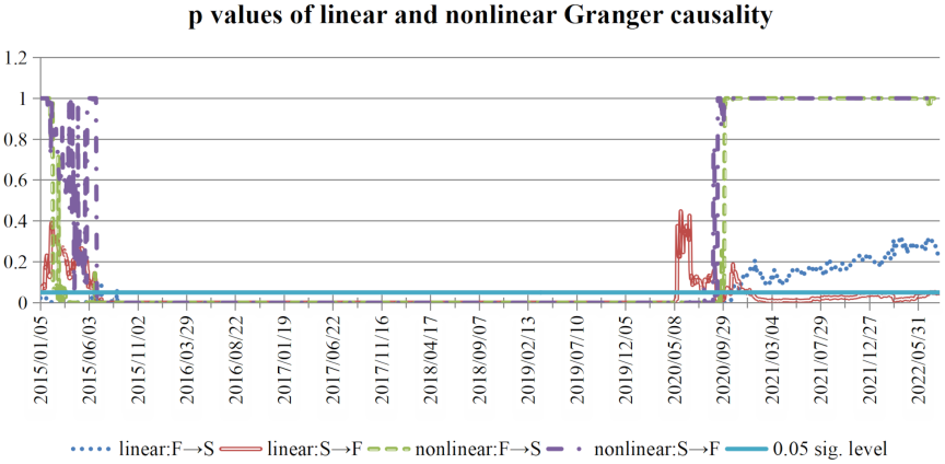
Fig. 1. \(p\)-values of linear and nonlinear causality tests for rolling samples (2015–2022).
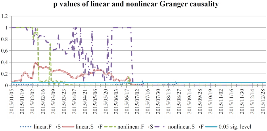
Fig. 2. \(p\)-values of linear and nonlinear causality tests for rolling samples (2015).
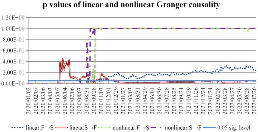
Fig. 3. \(p\)-values of linear and nonlinear causality tests for rolling samples (2020–2022).
5.3. Distributional Forecasting Granger Causality Test
5.3.1. Rolling Forecast Setup
Before implementing the rolling-window distributional forecasting procedure, we performed a preliminary model selection on the full sample to determine the appropriate lag order, volatility specification, and error distribution.
-
・
Lag-order selection: A VAR model was fitted to the bivariate return series \((S_t,F_t)\). Based on the SC, an optimal lag order of four was selected. This indicates that including up to four lags in each market’s return provides the best in-sample fit.
-
・
Volatility and distribution selection: For each market, we estimated GARCH(1,1) and EGARCH(1,1) models under three distributional assumptions: normal, Student-\(t\), and skewed-\(t\). The models were compared using the AIC and BIC. EGARCH(1,1), which exhibited a skewed-\(t\) distribution, consistently yielded the lowest information criteria, thus confirming its ability to capture the leverage effects, fat tails, and skewness typical of financial returns.
Based on these preliminary results, we adopted the following rolling forecast setup:
-
・
Mean equation: The conditional mean was modeled as a function of lagged terms up to order four, including all first-order (linear) terms, second-order quadratic (squared) terms, and second-order cross-product terms (e.g., \(S_{t-i}\cdot S_{t-j}\), \(F_{t-i}\cdot F_{t-j}\), and \(S_{t-i}\cdot F_{t-j}\)). For the benchmark model (using only own-market information), the candidate set contained 14 variables (four linear lags, four squared lags, and six within-market cross-products). For the extended model (including other market’s information), the total number of candidate variables was 44. Variables were selected using the LASSO with a cross-validated penalty \(\lambda\).
-
・
Volatility equation: EGARCH(1,1) to capture volatility clustering and leverage effects.
-
・
Distributional assumption: Skewed-\(t\) distribution to accommodate fat tails and skewness.
-
・
Rolling forecast mechanism: The first estimation window was April 19, 2010 to December 31, 2014 (1143 trading days). Subsequently, the window was shifted forward one day at a time, thus generating 1845 one-step-ahead distribution forecasts for each model.
We compared the benchmark model (own-lags only) with the extended model (own lags \(+\) other market’s lags, including all linear, squared, and cross-product terms). If the extended model yields a statistically superior out-of-sample distributional forecast, then we conclude that the other market Granger-causes the target market distributionally.
5.3.2. Test Based on PIT
We applied the PIT to the 1845 one-step-ahead forecast distributions derived from four models: S\(\sim\)S, S\(\sim\)S+F, F\(\sim\)F, and F\(\sim\)F+S. Fig. 4 presents the histograms and autocorrelation functions of the resultant PIT sequences, which shows no clear visual evidence of severe deviation from uniformity or substantial autocorrelation. The HL test 13 serves as a rigorous diagnostic verification. Under the null hypothesis of the correct model specification, the test statistic \(W\) and moment statistic \(M(i,j)\) asymptotically reflect the standard normal distribution, with a 5% critical value of 1.645.
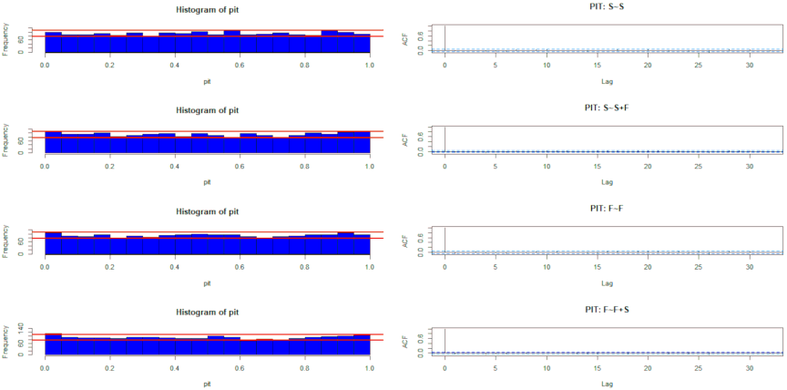
Fig. 4. Histograms and autocorrelation function plots of PIT sequences for each model.
Table 7 presents the HL test results. For spot forecasting, the benchmark model S\(\sim\)S yielded a significant \(W(4.002)\), thus indicating misspecification. After incorporating futures information (S\(\sim\)S+F), \(W\) declined to 0.721 (insignificant), whereas the second-moment statistic \(M(2,2)\) improved from 2.531 to \(-0.419\). For futures forecasting, the benchmark F\(\sim\)F indicated a significant \(W(2.517)\); incorporating spot information (F\(\sim\)F+S) reduced \(W\) to 2.252, with clear improvement in \(M(1,1)\) (from 2.974 to 0.267). These results confirm that including another market’s information significantly improves the specification of the conditional return distribution, particularly its volatility component.
| Model | \(M(1,1)\) | \(M(2,2)\) | \(M(3,3)\) | \(M(4,4)\) | \(M(1,2)\) | \(M(2,1)\) | \(W\) statistic |
| S\(\sim\)S | 1.148 | 2.531 | 1.605 | 0.432 | 0.266 | 4.682 | 4.002 |
| S\(\sim\)S+F | -0.597 | -0.419 | -1.041 | -1.679 | -1.796 | 1.538 | 0.721 |
| F\(\sim\)F | 2.974 | 0.717 | -0.918 | -1.759 | 0.448 | 3.992 | 2.517 |
| F\(\sim\)F+S | 0.267 | -1.513 | -0.665 | -1.715 | -0.923 | 1.291 | 2.252 |
| Note: Bold numbers indicate rejection of null hypothesis at 5% significance level (critical value of approximately 1.645). | |||||||
5.3.3. Test Based on Logarithmic Scoring Rule
As a complementary evaluation criterion, we employed the logarithmic scoring rule and the associated AG test 14. Based on the definitions in Section 3.3.4, the logarithmic score \(\mathit{LS}_t=\ln f_{t\mid t-1}(y_t)\) measures the accuracy of each density forecast, with lower values indicating better performance. For each pair of benchmark and extended models, we computed the score difference \(d_t=\mathit{LS}_t^{\,(\mathit{bench})}-\mathit{LS}_t^{\,(\mathit{ext})}\). The AG test examines whether the mean of \(d_t\) is significantly positive, which would imply that the extended model yields superior distributional forecasts.
Table 8 presents the average logarithmic scores over all rolling windows for the empirical period, in addition to the AG test \(p\)-values. The salient findings are as follows:
-
・
Spot market forecasting: The extended model S\(\sim\)S+F attains an average score of \(-1.625\), which is considerably higher (less negative) than \(-1.668\) of the benchmark S\(\sim\)S. The AG test \(p\)-value is \(1.660\times 10^{-16}\), which implies that the null of equal predictive accuracy should be rejected. Thus, adding futures information significantly improves the spot return distributional forecasts.
-
・
Futures market forecasting: Similarly, the extended model F\(\sim\)F+S yields an average score of \(-1.700\), thereby outperforming the benchmark F\(\sim\)F (\(-1.744\)). The AG test \(p\)-value is \(4.173\times 10^{-23}\), which is highly significant. Thus, spot information provides substantial incremental value for predicting the conditional distribution of futures returns.
| Empirical period | Robustness check period | |||
| Model | Avg. log score | AG test \(p\)-value | Avg. log score | AG test \(p\)-value |
| S\(\sim\)S | -1.668 | \(1.660 \times 10^{-16}\) | -1.633 | \(5.474 \times 10^{-27}\) |
| S\(\sim\)S+F | -1.625 | -1.620 | ||
| F\(\sim\)F | -1.744 | \(4.173 \times 10^{-23}\) | -1.647 | \(1.571 \times 10^{-24}\) |
| F\(\sim\)F+S | -1.700 | -1.635 | ||
These results are consistent with the HL test findings described in Section 5.3.2. Collectively, they provide robust evidence of bidirectional Granger causality in the distributional sense: historical information from one market not only aids one in specifying the correct conditional distribution of the other market (HL test) but also delivers economically meaningful improvements in out-of-sample predictive accuracy (AG test). The magnitude of the log-score gains (approximately 0.04 for both markets) is non-negligible, particularly in the context of financial risk management, where accurate density forecasts are critical for tail-risk assessment and portfolio optimization.
5.4. Information-Transmission Paths and Nonlinear Pattern Analysis
5.4.1. Variable Importance Measurement
To identify the lagged variables that contribute persistently to distributional forecasting, this study employed two complementary indicators:
-
(1)
Selection frequency (\(\boldsymbol{\mathit{SI}}_{\boldsymbol{i}}\)): The proportion of rolling windows in which variable \(\textrm{i}\) is selected by the LASSO estimation, thus reflecting its stability.
\begin{equation} \mathit{SI}_{i} = \dfrac{1}{T}\sum_{t=1}^{T} I\left(\hat{\beta}_{i,t}\ne 0\right), \label{eq:14} \tag{14} \end{equation}where \(T=1845\) denotes the total number of rolled windows. A higher \(\mathit{SI}_i\) value indicates that the variable is an effective predictor by the model across most market states.
-
(2)
Conditional coefficient mean \(\boldsymbol{\vert\bar{\beta}\vert_{i}^{\textit{cond}}}\): The average absolute value of the standardized regression coefficient of variable \(i\) over the windows in which it is selected, thus reflecting its average marginal contribution strength when active.
\begin{equation} \left\vert\bar{\beta}\right\vert_i^{\mathit{cond}} = \dfrac{1}{T_i}\sum_{\hat{\beta}_{{i,t}\ne 0}} \left\vert\hat{\beta}_{i,t}\right\vert, \label{eq:15} \tag{15} \end{equation}where \(T_i\) is the number of times variable \(i\) is selected. Because all variables are standardized before LASSO estimation, the coefficients of the different variables are comparable.
The two indicators capture the importance from different dimensions: a high \(\mathit{SI}_i\) indicates persistent and stable predictive information, and a high \(\vert\bar{\beta}\vert_i^{\mathit{cond}}\) indicates strong influence when selected. Combining both enables a more comprehensive identification of core transmission paths. Herein, variables with \(\mathit{SI}_i>0.8\) are defined as “important variables,” and their conditional coefficient means are reported.
5.4.2. Identification Results of Important Lagged Variables
| Model | Number of important variables | Important variables | \(\mathit{SI}_i\) | \(|\bar{\beta}|_{i}^{\mathit{cond}}\) |
| S\(\sim\)S | 2 | \(S_{t-4}\) | 0.9306 | 0.0671 |
| \(S_{t-2}\cdot S_{t-3}\) | 0.8455 | 0.0306 | ||
| S\(\sim\)S+F | 3 | \(F_{t-3}\) | 0.9447 | 0.0798 |
| \(F_{t-4}\) | 0.9144 | 0.0509 | ||
| \(S_{t-1}^2\) | 0.9783 | 0.0512 | ||
| F\(\sim\)F | 3 | \(F_{t-3}\) | 0.9447 | 0.0551 |
| \(F_{t-4}\) | 0.9263 | 0.0678 | ||
| \(F_{t-1}^2\) | 0.9534 | 0.0145 | ||
| F\(\sim\)F+S | 5 | \(F_{t-3}\) | 0.9745 | 0.1535 |
| \(F_{t-4}\) | 0.9680 | 0.0554 | ||
| \(S_{t-1}^2\) | 0.9474 | 0.0966 | ||
| \(S_{t-1}\cdot F_{t-4}\) | 0.9344 | 0.0721 | ||
| \(S_{t-3}\cdot S_{t-4}\) | 0.9631 | 0.1286 |
Based on the method above, the important variables identified for the four forecasting models during the empirical period are listed in Table 9. All the selected variables have selection frequencies above 0.84, with most exceeding 0.93, thus indicating that these lagged terms provide persistently stable contributions to distributional forecasting.
-
(1)
Spot-only model (S\(\boldsymbol{\sim}\)S): Two variables are important: the linear term \(S_{t-4}\) (\(\mathit{SI}=0.9306\), \(\vert\bar{\beta}\vert^{\mathit{cond}}=0.0671\)) and the nonlinear product term \(S_{t-2}\cdot S_{t-3}\) (\(\mathit{SI}=0.8455\), \(\vert\bar{\beta}\vert^{\mathit{cond}}=0.0306\)). The relatively modest coefficients suggest that spot returns exhibit mild linear autocorrelation at lag 4 and a weak but persistent nonlinear interaction between lags 2 and 3.
-
(2)
Spot model with futures information (S\(\boldsymbol{\sim}\)S\(\boldsymbol{+}\)F): Futures lags \(F_{t-3}\) (\(\mathit{SI}=0.9447\), \(\vert\bar{\beta}\vert^{\mathit{cond}}=0.0798\)) and \(F_{t-4}\) (\(\mathit{SI}=0.9144\), \(\vert\bar{\beta}\vert^{\mathit{cond}}=0.0509\)) enter the important set, while the squared spot term \(S_{t-1}^2\) (\(\mathit{SI}=0.9783\), \(\vert\bar{\beta}\vert^{\mathit{cond}}=0.0512\)) remains highly relevant. This confirms that futures lead spots with a lag of three to four periods and that nonlinear volatility persistence in the spot market remains relevant even after futures information is controlled.
-
(3)
Futures-only model (F\(\boldsymbol{\sim}\)F): The important variables are \(F_{t-3}\) (\(\mathit{SI}=0.9447\), \(\vert\bar{\beta}\vert^{\mathit{cond}}=0.0551\)), \(F_{t-4}\) (\(\mathit{SI}=0.9263\), \(\vert\bar{\beta}\vert^{\mathit{cond}}=0.0678\)) and \(F_{t-1}^2\) (\(\mathit{SI}=0.9534\), \(\vert\bar{\beta}\vert^{\mathit{cond}}=0.0145\)). The small coefficient of the quadratic term indicates that the futures market dynamics are predominantly linear.
-
(4)
Futures model with spot information (F\(\boldsymbol{\sim}\)F\(\boldsymbol{+}\)S): Five variables are important: futures lags \(F_{t-3}\) (\(\mathit{SI}=0.9745\), \(\vert\bar{\beta}\vert^{\mathit{cond}}=0.1535\)) and \(F_{t-4}\) (\(\mathit{SI}=0.9680\), \(\vert\bar{\beta}\vert^{\mathit{cond}}=0.0554\)); the squared spot term \(S_{t-1}^2\) (\(\mathit{SI}=0.9474\), \(\vert\bar{\beta}\vert^{\mathit{cond}}=0.0966\)); the cross-product \(S_{t-1}\cdot F_{t-4}\) (\(\mathit{SI}=0.9344\), \(\vert\bar{\beta}\vert^{\mathit{cond}}=0.0721\)); and the nonlinear product \(S_{t-3}\cdot S_{t-4}\) (\(\mathit{SI}=0.9631\), \(\vert\bar{\beta}\vert^{\mathit{cond}}=0.1286\)). These results reveal that spot-market information exerts a strong and fast (lag-1) influence on futures returns through both linear (\(S_{t-1}\) implied by the cross-product and the large coefficient on \(F_{t-3}\) may capture indirect effects as well) and nonlinear channels. The high conditional coefficients for \(F_{t-3}\) (0.1535) and \(S_{t-3}\cdot S_{t-4}\) (0.1286) indicate that the spot-to-futures transmission is generally larger in magnitude than the reverse direction.
Collectively, the evidence supports the study’s two main conclusions: (i) A robust bidirectional nonlinear time-varying price-discovery process exists, and (ii) cross-market leadership is dominated by linear spillovers (e.g., \(F_{t-3}\) and \(F_{t-4}\)), while nonlinear effects (squared and product terms) are primarily internalized within each market’s own volatility structure.
5.4.3. Economic Implications and Strategy Insights
The identified transmission paths reveal a “dual-track asynchronous” price-discovery pattern: futures affect spot with a lag of three to four periods, whereas spots affect futures with a rapid one-period impact and sustained feedback at lags 3–4. Moreover, the spot-to-futures coefficients are generally larger (up to 0.1286) than the futures-to-spot coefficients (up to 0.0798), thus indicating that the spot market is the dominant pricing anchor.
Why do futures lead spot with a lag of three to four days? This seemingly counterintuitive finding can be explained by three interaction mechanisms. First, daily price limits in the Chinese A-share market (\(\pm 10\%\)) prevent spot prices from fully absorbing extreme information on the same day. When futures prices shift significantly (e.g., by –3%), the spot market may reach the limit, thus causing the price adjustment to continue over the following three to four trading days 18. Second, the retail-dominated investor structure (individual investors account for a large proportion of trading volume) results in slower information diffusion. Professional traders react to futures signals first, followed by retail investors, who require time for confirmation and herding, thus creating a multiday cascade 19. Third, arbitrage constraints. Short selling in the spot market is costly and operationally complex, thus limiting the ability of arbitrageurs to immediately eliminate mispricing and allowing the price discrepancy to persist for several days 20. These institutional and behavioral factors simultaneously result in an observable 3–4 day lag, which is not a failure of market efficiency but rather a reflection of the market microstructure in an emerging market.
Practical implications. For dynamic hedging, portfolio managers should focus on futures returns and spot-market volatility at lags 3–4 and 1, respectively, thus expanding beyond conventional same-day or lag-1 models. The dominance of linear mean spillovers in cross-market transmission suggests that relatively simple linear models may be sufficient for constructing real-time cross-market risk monitoring systems. Finally, the persistent presence of the squared spot term \(S_{t-1}^2\) in both spot and futures models indicates that volatility forecasting should incorporate own-market nonlinear dynamics, even when other-market information is included.
5.5. Robustness Verification
5.5.1. Changing Sample Period (Excluding 2010–2013)
To assess whether the main conclusions are affected by the sample period, we repeated the analysis using a subsample that excluded the early market phase (2010–2013). The rationale is that the CSI 300 index futures were launched in April 2010. During the first few years, the market might have been affected by low liquidity, an immature investor base, and ongoing mechanism adjustments, which might have temporarily affected the price-discovery process. Focusing on the more mature period from 2014 onwards provides a clearer environment for examining the intrinsic futures–spot leadership relationship.
The HL test results for this subsample (Table 10) show that the benchmark models (S\(\sim\)S, F\(\sim\)F) remain misspecified (significant \(W\) statistics), whereas the extended models (S\(\sim\)S+F, F\(\sim\)F+S) yield insignificant \(W\) statistics, thereby indicating correctly specified forecast distributions. The AG test (Table 8, right column) confirms that the extended models significantly outperform the benchmarks (\({p<0.01}\)). Moreover, the important lagged variables identified in the robustness sample (Table 11) are nearly identical to those in the full sample, with \(F_{t-3}\), \(F_{t-4}\), \(S_{t-1}\), \(S_{t-1}^2\) remaining as the core drivers. Thus, the bidirectional distributional causality and specific transmission paths are not artifacts of the sample period.
| Model | \(M(1,1)\) | \(M(2,2)\) | \(M(3,3)\) | \(M(4,4)\) | \(M(1,2)\) | \(M(2,1)\) | \(W\) statistic |
| S\(\sim\)S | 1.8742 | 2.9101 | 1.7878 | 0.3279 | 1.2737 | 3.8073 | 1.7305 |
| S\(\sim\)S+F | 0.4427 | 1.0077 | 0.3438 | -0.5924 | -0.3951 | 1.5978 | 0.2306 |
| F\(\sim\)F | 1.8038 | 1.9236 | 0.6871 | -0.4916 | 1.4372 | 2.6826 | 0.6032 |
| F\(\sim\)F+S | 0.5470 | 0.4488 | -0.3946 | -1.2202 | -0.1589 | 1.4669 | 1.2517 |
| Note: Bold numbers indicate rejection of null hypothesis at 5% significance level. | |||||||
| Model | Number of important variables | Important variables |
| S\(\sim\)S | 1 | \(S_{t-2}\cdot S_{t-3}\) |
| S\(\sim\)S+F | 5 | \(F_{t-3}\), \(F_{t-4}\), \({F_{t-3}\cdot F_{t-4}}\), \(S_{t-1}^2\), \({S_{t-1}\cdot F_{t-4}}\) |
| F\(\sim\)F | 5 | \(F_{t-3}\), \(F_{t-4}\), \(F_{t-1}^2\), \({F_{t-1}\cdot F_{t-4}}\), \({F_{t-3}\cdot F_{t-4}}\) |
| F\(\sim\)F+S | 6 | \(F_{t-3}\), \(F_{t-4}\), \(S_{t-1}^2\), \({S_{t-1}\cdot F_{t-4}}\), \({S_{t-3}\cdot S_{t-4}}\), \({S_{t-3}\cdot F_{t-4}}\) |
5.5.2. Additional Remarks
Several other potential concerns are addressed through theoretical arguments instead of additional computations:
-
・
Multi-step-ahead forecasting: Granger causality was originally defined for one-step-ahead prediction 12. Multistep forecasts from the EGARCH models accumulate nonlinear errors, which can distort inferences. Moreover, our analysis captures medium-term effects (3–4 day lags) through the lag structure in the mean equation (see Table 9). Therefore, we focus on the one-step-ahead forecasts, which are consistent with the theoretical definition.
-
・
Different lag orders (e.g., six or eight): The lag order of four was selected by the SC on the full sample. Nevertheless, the LASSO automatically excludes irrelevant longer lags if they do not contribute to predictive accuracy. Thus, increasing the maximum lag order would not alter the selection of the important variables identified in Table 9.
-
・
Alternative volatility models or error distributions: The preliminary model selection in Section 5.3.1 identified EGARCH with skewed-\(t\) as the optimal specification based on the AIC and BIC. Furthermore, the Monte Carlo simulations in Section 4 show that the proposed test maintains desirable finite-sample properties even under the more restrictive GARCH-normal setting. Consequently, deviations from the optimal specifications are unlikely to overturn our conclusions. Hence, we did not conduct additional robustness verifications beyond the sample-period change. The results reported in Sections 5.2–5.4 are thus reliable and robust to a range of reasonable alternatives.
6. Conclusions
In this study, a novel Granger causality testing framework was developed based on distributional forecasting and then applied to investigate the price-leadership mechanism between China’s CSI 300 stock index futures and spot markets. Unlike conventional tests that focus on conditional expectations or specific quantiles, the proposed framework compares the entire out-of-sample conditional distribution of returns with and without another market’s information. It integrates a nonlinear mean equation (LASSO with linear, quadratic, and cross-product terms), a time-varying volatility model (EGARCH), and strict forecast evaluation using PIT-based HL tests and logarithmic-score AG tests within a rolling-window scheme.
Monte Carlo simulations validated the finite-sample properties of the test: the empirical size remained close to the nominal 5% level, whereas the power exceeded 0.94 for linear causality and 0.83 for nonlinear causality under moderate sample sizes. This demonstrated the reliability of the test for empirical applications.
By applying this framework to daily data from April 2010 to August 2022, we obtained several key findings. First, robust bidirectional nonlinear time-varying Granger causality existed between the two markets. Classical linear tests capture only spot-to-future leadership, whereas nonlinear tests reveal a two-way interaction. Second, the distributional forecasting causality test showed that including cross-market information significantly improved the out-of-sample forecasts of the entire return distribution for both markets. Third, we identified specific transmission paths: futures led spots through linear signals at lags 3 and 4, whereas spots led futures through a rapid one-period impact (lag 1) and sustained feedback at lags 3 and 4. The effect from spot to futures was greater compared with that in the reverse direction. Fourth, linear spillovers dominated cross-market transmission, whereas nonlinear effects (squared and product terms) were primarily internalized within each market’s volatility structure. The seemingly counterintuitive 3–4 days lag from futures to spot is attributable to institutional and behavioral mechanisms: daily price limits, a retail-dominated investor structure, and arbitrage constraints, all of which are characteristic of China’s emerging financial market.
This study offers three major contributions to the literature. Methodologically, it returns to Granger’s original distributional forecasting definition and provides a practical, computationally feasible testing procedure that can be applied to any pair of financial time series where whole-distribution predictability is important. Empirically, it uncovers a “dual-track asynchronous” pattern of price discovery in China’s index futures market, with distinct lag structures and asymmetric leadership strengths. Practically, the findings offer concrete guidance for dynamic hedging (focusing on futures lags 3–4 and spot volatility at lag 1) and for building parsimonious cross-market risk-monitoring systems that rely on linear mean spillovers.
Nonetheless, this study has several limitations. First, the analysis uses daily data and cannot capture intraday dynamics; high-frequency data can reveal even finer lead-lag relationships. Second, the distributional assumption is parametric (skewed-\(t\)); nonparametric or machine learning-based density forecasts may further improve performance. Third, the framework can be extended to other index futures (CSI 500 and CSI 1000) and to other asset classes (commodities and currencies). Finally, incorporating external information, such as market or news sentiment, can enrich the information set. In general, the distributional forecasting Granger causality framework provides an effective and flexible tool for analyzing complex dynamic linkages in financial markets.
Acknowledgments
This study was supported by the National Social Science Foundation of China (Grant Number 25BJY029).
Footnotes
(1) Results of LASSO regression are relatively complex and thus not presented individually herein. They are available from the authors upon request.
- [1] C. He, L. Zhang, and W. Chen, “Research on Price Discovery of HS300 Index Futures Based on High Frequencies Data,” J. Quant. Tech. Econ., Vol.28, No.5, pp. 139-151, 2011 (in Chinese). https://doi.org/10.13653/j.cnki.jqte.2011.05.010
- [2] J. Yang, Z. Yang, and Y. Zhou, “Intraday price discovery and volatility transmission in stock index and stock index futures markets: Evidence from China,” J. Futures Mark., Vol.32, No.2, pp. 99-121, 2012. https://doi.org/10.1002/fut.20514
- [3] K. Fang and Z. Cai, “Research on price discovery function of stock index futures in Chinese emerging market,” Stat. Res., Vol.29, No.5, pp. 73-78, 2012 (in Chinese). https://doi.org/10.19343/j.cnki.11-1302/c.2012.05.010
- [4] H. Zhao, X. Chen, and S. Huang, “Difference of information transmission between the Chinese stock and index futures markets,” Syst. Eng. Theory Pract., Vol.38, No.4, pp. 863-872, 2018 (in Chinese). https://doi.org/10.12011/1000-6788(2018)04-0863-10
- [5] Z. Li, L. Bu, and Y. Hao, “Further discussion on price discovery function of Chinese stock index futures—Evidence from three listed species,” Financ. Trade Econ., Vol.2016, No.7, pp. 79-93, 2016 (in Chinese). https://doi.org/10.19795/j.cnki.cn11-1166/f.2016.07.006
- [6] A. Ghedira and M. S. Nakhli, “Dynamic causality between oil prices and stock market indexes in Russia and China: Does US financial instability matter?,” Int. J. Emerg. Mark., Vol.19, No.11, pp. 4186-4203, 2024. https://doi.org/10.1108/IJOEM-06-2022-1018
- [7] C. Diks and V. Panchenko, “A new statistic and practical guidelines for nonparametric Granger causality testing,” J. Econ. Dyn. Control, Vol.30, Nos.9-10, pp. 1647-1669, 2006. https://doi.org/10.1016/j.jedc.2005.08.008
- [8] N. Qiu, “General causality test based on improvement of Lasso,” Stat. Inf. Forum, Vol.2008, No.2, pp. 18-21+36, 2008 (in Chinese).
- [9] X. Ren and W. Sun, “Asymmetric risk spillovers between the chinese stock market and index futures market based on Granger non-causality test in quantiles,” Oper. Res. Manag. Sci., Vol.30, No.8, pp. 190-197, 2021 (in Chinese).
- [10] M. J. Kim and S. Y. Park, “Quantile causal relationship between Bitcoin and stock indices,” J. Asia Pac. Econ., Vol.30, No.3, pp. 812-828, 2025. https://doi.org/10.1080/13547860.2024.2347481
- [11] J. Zhang, J. Zhao, and C. C. Lee, “Asymmetric dynamics between cryptocurrency uncertainty and the oil and gold markets: Evidence from Granger causality in quantiles,” Appl. Econ., Vol.57, No.7, pp. 709-722, 2025. https://doi.org/10.1080/00036846.2024.2305618
- [12] C. W. J. Granger, “Investigating causal relations by econometric models and cross-spectral methods,” Econometrica, Vol.37, No.3, pp. 424-438, 1969. https://doi.org/10.2307/1912791
- [13] Y. Hong and H. Li, “Nonparametric specification testing for continuous-time models with applications to term structure of interest rates,” Rev. Financ. Stud., Vol.18, No.1, pp. 37-84, 2005. https://doi.org/10.1093/rfs/hhh006
- [14] G. Amisano and R. Giacomini, “Comparing density forecasts via weighted likelihood ratio tests,” J. Bus. Econ. Stat., Vol.25, No.2, pp. 177-190, 2007. https://doi.org/10.1198/073500106000000332
- [15] C. W. J. Granger, “Some properties of time series data and their use in econometric model specification,” J. Econom., Vol.16, No.1, pp. 121-130, 1981. https://doi.org/10.1016/0304-4076(81)90079-8
- [16] Y. Fang and X. W. Xie, “Research on nonlinear linkage effects in China’s multi-level capital markets: Also on the maturity of capital markets,” Econ. Sci., No.3, pp. 72-84, 2014 (in Chinese). https://doi.org/10.19523/j.jjkx.2014.03.006
- [17] H. Liu and L. He, “The spatial network structure of China’s provincial economic growth: Reexamination based on nonlinear Granger causality test,” J. Financ. Econ., Vol.42, No.2, pp. 97-107, 2016 (in Chinese). https://doi.org/10.16538/j.cnki.jfe.2016.02.009
- [18] R. M. Xue, “The impact of price limit system on Shanghai and Shenzhen stock markets,” Master’s thesis, North China University of Technology, 2009 (in Chinese).
- [19] B. M. Barber and T. Odean, “All that glitters: The effect of attention and news on the buying behavior of individual and institutional investors,” Rev. Financ. Stud., Vol.21, No.2, pp. 785-818, 2008. https://doi.org/10.1093/rfs/hhm079
- [20] A. Shleifer and R. W. Vishny, “The limits of arbitrage,” J. Financ., Vol.52, No.1, pp. 35-55, 1997. https://doi.org/10.1111/j.1540-6261.1997.tb03807.x
This article is published under a Creative Commons Attribution-NoDerivatives 4.0 Internationa License.