
Research Paper:
Entropies and Negentropies from f-Divergences and Their Application to Dimensionality Reduction
Mateu Sbert*1
 , Min Chen*2
, Jordi Poch*1
, Miquel Feixas*1
, Shuning Chen*3
, and Víctor Elvira*4
, Min Chen*2
, Jordi Poch*1
, Miquel Feixas*1
, Shuning Chen*3
, and Víctor Elvira*4
*1University of Girona
Plaça Sant Domènec, 3, Girona 17004, Spain
*2University of Oxford
Oxford e-Research Centre, 7 Keble Road, Oxford OX 3, United Kingdom
*3Hiroshima University
1-5-1 Kagamiyama, Higashi-Hiroshima, Hiroshima 739-8529, Japan
*4School of Mathematics, University of Edinburgh
James Clerk Maxwell Building, Peter Guthrie Tait Road, Edinburgh EH 3, United Kingdom

Distributions are ubiquitous across scientific disciplines, extending well beyond probability and statistics. In machine learning, finite probability distributions arise naturally as the softmax output layers of convolutional neural networks and large language models, where they encode class probabilities in image classification and token probabilities in language generation. When such distributions are high dimensional, however, storage and computational costs become significant. In previous work, we introduced two families of generalized entropies derived from f-divergences, using majorization as a reference framework for comparing distributional homogeneity. In this paper, we extend that framework in several directions. First, we study majorization relationships between subcompositions of a distribution. Second, we introduce generalized negentropies derived from f-divergences and analyze their role alongside entropies in dimensionality reduction. Third, we embed both entropies and negentropies into the setting of Shannon’s information channel and show that the classical channel identities are satisfied exclusively by Shannon entropy. These results provide a unified information-theoretic framework for dimensionality reduction of finite distributions, clarifying the structural role of f-divergence-based entropies and negentropies and their relation to classical information measures.
1. Introduction
Finite distributions play a central role not only in probability and statistics but across nearly all scientific disciplines. In machine learning, distributions are indispensable: they underpin the softmax output layers of convolutional neural networks and large language models, where they model categorical probabilities that are fundamental to image classification and language generation 1,2. As the dimensionality of these distributions increases, however, both storage requirements and computational costs grow accordingly.
Quantifying the homogeneity, diversity, or concentration of a distribution is therefore of practical and theoretical importance in a wide range of applications, including the analysis of wealth distributions 3, the assessment of sampling efficiency 4, and the evaluation of biodiversity 5. Shannon entropy and its classical generalizations, such as those of Rényi 6 and Tsallis 7, have long been used as diversity indices. Since entropy can be interpreted as the information content of a distribution 8, it is natural to seek dimensionality reduction procedures that preserve entropy or information as much as possible.
In previous work 9, we introduced two families of generalized entropies derived from \(f\)-divergences, using majorization as a principled baseline for comparing distributional homogeneity 10,11,12. Building on earlier research on level of detail and refinement criteria 13,14,15,16, these entropies were subsequently applied to dimensionality reduction and embedded into an information-theoretic framework related to Shannon’s information channel in 17.
The present paper extends this line of research in several directions. First, we examine majorization relations between subcompositions of a distribution, providing a finer structural analysis of how grouping operations affect homogeneity. Second, we introduce generalized negentropies derived from \(f\)-divergences and study their interaction with entropies in dimensionality reduction tasks. Unlike entropies, these negentropies explicitly capture deviations from uniformity and allow for complementary simplification criteria that explicitly account for alphabet size. Third, we analyze the role of both entropies and negentropies within the framework of Shannon’s information channel and prove that the classical channel identities hold if and only if the entropy is Shannon’s.
The remainder of the paper is organized as follows. Section 2 reviews \(f\)-divergences. Section 3 recalls the majorization order and Schur convexity. Section 4 introduces the generalized entropies. Section 5 studies dimensionality reduction for a single distribution, while Section 6 addresses dimensionality reduction in the presence of joint and conditional distributions and discusses the analogy with Shannon’s information channel. Section 7 introduces generalized negentropies derived from \(f\)-divergences. Section 8 presents and discusses illustrative simplification examples, and Section 9 concludes.
2. \(f\)-Divergences
The \((n-1)\)-simplex \(S_{n-1}\) consists of all convex combinations of the \(n\) vertices \((1,0,\ldots,0)\), \((0,1,0,\ldots,0)\), …, \((0,\ldots,0,1)\).
The \(f\)-divergence \(D_f(p,q)\) between two probability distributions \(p\) and \(q\) in \(S_{n-1}\) is defined as
The condition \(f(1)=0\) ensures non-negativity. Indeed, by Jensen’s inequality 8,
We adopt the standard conventions \(0f(0/0)=0\) and, for \(a>0\), \(0f(a/0) = \lim_{t \to 0^{+}} tf(a/t)\), which ensure that \(D_{f}(p,q) = D_{f}(\{p, 0\}, \{q, 0\})\).
From the definition, \(D_{f}(p,q)\) is invariant under permutations of indices and satisfies the following properties:
-
・
\(D_{f}(p,q)\ge0\), with equality at \(p=q\); if \(f\) is strictly convex, equality implies \(p=q\);
-
・
\(D_{f}(p,q)\) is jointly convex in \((p,q)\);
-
・
\(D_{f}(p,q)\equiv D_{f(x)+c(x-1)}(p,q)\) for any constant \(c\);
-
・
\(D_{f}(p,q)\ge D_f(pT,qT)\) for any stochastic matrix \(T\) (data-processing inequality). In particular, \(T\) may represent a clustering of indices.
Well-known examples of \(f\)-divergences include
-
・
the Kullback–Leibler (KL) divergence \(\mathrm{KL}(p,q) = \sum_{i} p_{i} \log (p_{i}/q_{i})\), with \(f(x) = x \log x\),
-
・
the total variation distance \(\mathrm{TV}(p,q) = (1/2)\sum_{i} |p_{i}-q_{i}|\), with \(f(x) = (1/2)|x-1|\), which is the only \(f\)-divergence that is also a metric induced by a norm,
-
・
the squared Hellinger distance \(H^{2}(p,q) = \sum_{i}(\sqrt{p_{i}}-\sqrt{q_{i}})^{2}\), with \(f(x) = (\sqrt{x}-1)^{2}\), and
-
・
the \(\chi^{2}\)-divergence \(\chi^{2}(p,q) = \sum_{i} (p_{i}-q_{i})^{2}/q_{i}\), with \(f(x) = (x-1)^{2}\).
Another important example is the one-parameter family of Tsallis \(f\)-divergences, defined for \(\alpha>0\) and \(\alpha\neq1\) by \(f(x) = (x^{\alpha}-1)/(\alpha-1)\),
3. Majorization and Schur-Convexity
A doubly stochastic matrix \(\mathbf{T} = \{t_{ij}\}_{i,j=1}^{n}\) satisfies \(t_{ij} \ge 0\) for all \(i,j\) and
Definition 1. Given \(p,q \in S_{n-1}\), let \(p^{↓}\) and \(q^{↓}\) denote the vectors obtained by reordering the components of \(p\) and \(q\) in non-increasing order. We say that \(p\) majorizes \(q\), and write \(p\succ q\) (or equivalently \(q \prec p\)), if for all \(1 \le j \le n\),
The condition (3) is equivalent to the existence of a doubly stochastic matrix \(\mathbf{T}\) such that
Majorization defines a preorder on \(S_{n-1}\): it is transitive but not total, as there exist incomparable distributions, for instance \(\{0.6, 0.2, 0.2\}\) and \(\{0.5, 0.4, 0.1\}\). It is also not antisymmetric, since \(\{1, 0, 0\} \succ \{0, 1, 0\}\) and \(\{0, 1, 0\} \succ \{1, 0, 0\}\) while the two vectors are distinct.
The relation \(p \succ q\) can be checked either via the partial sums in Eq. (3) or by exhibiting a doubly stochastic matrix \(\mathbf{T}\) such that \(q = p\mathbf{T}\). For example, \(\{1/3, 2/3\} \succ \{4/9, 5/9\}\) since
A particularly relevant case is the grouping of indices. Given a distribution \(p=\{p_{1}, p_{2}, \ldots, p_{n}\}\), grouping \(p_1\) and \(p_2\) yields \(\{0, {p_{1}+p_{2}}, p_{3}, \dots, p_{n}\}\), and
A function \(E\colon S_{n-1} \to \mathbb{R}\) is Schur-convex (respectively, Schur-concave) 11 if and only if \(p\succ q\) implies \(E(p)\ge E(q)\) (respectively, \(E(p)\le E(q)\)). Shannon entropy \(H(p)=-\sum_{i} p_{i}\log p_{i}\) 8 is Schur-concave.
Let \(\mathbf{1}_n\) denote any permutation of \((1,0,\ldots,0)\) and let \(\mathbf{u}_{n} = (1/n,\ldots,1/n)\). Then for all \(p\in S_{n-1}\),
Since grouping any number of indices can be obtained by successive applications of Eq. (4), transitivity of majorization implies the following proposition:
Proposition 2 (Grouping property). For any distribution \(p\) and any Schur-concave function \(E\), if indices of \(p\) are grouped to obtain \(\{p',\mathbf{0}\}\), then \(E(p) \ge E(\{p',\mathbf{0}\})\).
Observe that whether the equality \(E(\{p',\mathbf{0}\}) = E(p')\) holds depends on the specific function \(E\).
4. Entropies from \(f\)-Divergences
In our previous work 9, we introduced two generalizations of Shannon entropy, denoted by \(E^{C{\&}A}_{f}(p)\) and \(E^{\mathit{Top}}_{f}(p)\), based on the approaches of Cichocki and Amari 21 and Topsøe 22, respectively. Both families are constructed from a convex function \(f\) satisfying \(f(1)=0\) and can, therefore, be naturally associated with the corresponding \(f\)-divergence \(D_{f}(p,q)\). As for \(f\)-divergences, both entropy definitions are invariant under the transformation \(f'(x)=f(x)+c(x-1)\), thus in 17, we added for convenience the condition \(f(0)=f(0^{+})=0\), obtained by shifting \(f(x)\) to \(f'(x)=f(x)-f(0)(x-1)\). Like Shannon entropy, \(E^{C{\&}A}_{f}(p)\) and \(E^{\mathit{Top}}_f(p)\) are concave and Schur-concave, vanish at \(\mathbf{1}_{n}\), and attain their maximum at the uniform distribution \(\mathbf{u}_{n}\).
This section establishes the structural properties of these two families that are directly relevant to dimensionality reduction. The two key questions we address here are (i) when do the two families coincide (Proposition 3), and (ii) when is an entropy invariant under the addition or removal of zero-probability symbols (Proposition 4). Both questions turn out to have the same answer: exclusively for Shannon entropy. This uniqueness result motivates the different treatment that \(E^{C{\&}A}_f\) and \(E^{\mathit{Top}}_f\) require in the simplification procedures of Sections 5–7: while \(E^{\mathit{Top}}_f\) is naturally compatible with the removal of empty bins (a standard step in any real grouping operation), \(E^{C{\&}A}_f\) is not, which ultimately drives the introduction of negentropies in Section 7.
4.1. \(E^{C{\&}A}_{f}(p)\) Entropies
Inspired by Cichocki and Amari 21, we defined in 9,17 the entropy
A remarkable property of \(E^{C{\&}A}_{f}(p)\) is that, in general
Consider first the Hellinger entropy (Table 1). For \(p \neq \mathbf{1}_{n}\),
| Divergence | \(f(x)\) | \(E^{C{\&}A}(p)\) | \(E^{C{\&}A}(\mathbf{u}_{n})\) |
| Generic | \(f(x)\) (\(f(1)=f(0)=0\)) | \((1/n)f(n) - \sum_{i=1}^{n}(1/n)f(np_{i})\) | \((1/n)f(n)\) |
| TV | \((1/2)|x-1| + (1/2)(x-1)\) | \((n-1)/n - (1/2)\sum_{i=1}^{n} |p_{i}-1/n|\) | \((n-1)/n\) |
| \(\chi^{2}\) | \(x^{2}-x\) | \(n(1-\sum_{i=1}^{n} p_{i}^{2})\) | \(n-1\) |
| KL (Shannon) | \(x \log x\) | \(-\sum_{i=1}^{n} p_{i} \log p_{i}\) | \(\log n\) |
| Hellinger | \(2x - 2\sqrt{x}\) | \((2/\sqrt{n}) (\sum_{i=1}^{n} \sqrt{p_{i}} - 1)\) | \(2(1 - 1/\sqrt{n})\) |
| Tsallis | \((x^{\alpha}-x)/(\alpha-1)\) | \((1/(n(\alpha-1))) (1+ n^{\alpha-1} - \sum_{i=1}^{n}(np_{i})^{\alpha})\) | \((1/(\alpha-1))(n^{\alpha-1}-1)\) |
| Jensen-Shannon | \(\begin{aligned}[t] f(x) &= (x+1) \log (2/(x+1)) \\ & +x \log x+ (x-1) \log 2 \end{aligned}\) | \(\begin{aligned}[t] 2 \log 2 &+ \log n - ((n+1)/n) \log (n+1) \\ &- (1/n)\textstyle\sum_{i=1}^{n} ((np_{i}+1) \log(2/(np_{i}+1)) \\ & + np_{i} \log np_{i}) \end{aligned}\) | \(\begin{aligned}[t] 2 \log 2+ \log n - ((n+1)/n)\log (n+1) \end{aligned}\) |
| Divergence | \(f(x)\) | \(E^{\mathit{Top}}(p)\) | \(E^{\mathit{Top}}(\mathbf{u}_{n})\) |
| Generic | \(f(x)\) (\(f(1)=f(0)=0\)) | \(-\sum_{i=1}^{n} f(p_{i})\) | \(-nf(1/n)\) |
| TV | \((1/2)|x-1| + (1/2)(x-1)\) | 0 | 0 |
| \(\chi^{2}\) | \(x^{2}-x\) | \(1-\sum_{i=1}^{n} p_{i}^{2}\) | \(1-1/n\) |
| KL (Shannon) | \(x \log x\) | \(-\sum_{i=1}^{n} p_{i} \log p_{i}\) | \(\log n\) |
| Hellinger | \(2x-2\sqrt{x}\) | \(2(\sum_{i=1}^{n}\sqrt{p_{i}}-1)\) | \(2(\sqrt{n}-1)\) |
| Tsallis | \((x^{\alpha}-x)/(\alpha-1)\) | \((1/(\alpha-1))(1-\sum_{i=1}^{n}p_{i}^{\alpha})\) | \((1/(\alpha-1))(1-n^{1-\alpha})\) |
| Jensen-Shannon | \(\begin{aligned}[t] f(x) = &(x+1)\log(2/(x+1)) \\ & + x \log x +(x-1) \log 2 \end{aligned}\) | \(-2 \log 2+\sum_{i=1}^{n}((p_i+1)\log(p_{i}+1) -p_{i} \log p_{i})\) | \(-2 \log 2+(n+1)\log ((n+1)/n) + \log n\) |
4.2. \(E^{\mathit{Top}}_{f}(p)\) Entropies
Following Topsøe 22, we defined in 9,17
In contrast to \(E^{C{\&}A}_{f}(p)\), we have \(E^{\mathit{Top}}_{f}(p) = E^{\mathit{Top}}_{f}(\{p,0\})\). Consequently, if \(p\) is grouped into \(\{p',\mathbf{0}\}\), Proposition 2 implies
Proposition 3. \(E^{\mathit{Top}}_{f}(p) \equiv E^{C{\&}A}_{f}(p)\) if and only if \(f(x) = cx\log x\), with \(c\ge 0\).
Proof. The direct implication is immediate. Conversely, consider \(p = \{x, {1-x}, 0, \ldots, 0\}\in S_{n-1}\). If \(E^{\mathit{Top}}_{f}(p) = E^{C{\&}A}_{f}(p)\), then, for all \(n\ge2\),
Proposition 4. \(E^{C{\&}A}_{f}(p) = E^{C{\&}A}_{f}(\{p,0\})\) for all \(p\) if and only if \(f(x) = cx\log x\).
Proof. Equating the entropies of \(\{x,{1-x}\}\) and \(\{x,{1-x},0,\ldots,0\}\in S_{n-1}\) yields
Differentiating both sides gives
Examples of both \(E^{C{\&}A}_{f}(p)\) and \(E^{\mathit{Top}}_{f}(p)\) entropies associated with well-known \(f\)-divergences are listed in Table 1, where \(f(x)\) has been normalized so that \(f(0)=0\). Note that the \(E^{\mathit{Top}}_{f}(p)\) entropy associated with total variation degenerates to zero. For \(f(x)=x\log x\), both definitions reduce to Shannon entropy.
5. Reducing Dimensionality
5.1. Task Definition
Throughout Sections 5–7, the dimensionality reduction task is defined as follows.
Variable and distributions. We consider a discrete random variable \(X\) with \(n\) symbols and probability distribution \(p(X)\in S_{n-1}\). When a joint distribution \(p(X,Y)\) is also given (Sections 6–7), \(Y\) has \(m\) symbols and is kept fixed; only \(X\) is simplified.
Operations. The two elementary simplification operations are:
-
・
Merging (grouping): one of the two symbols, denoted \(x'\), absorbs the other: \(p(x')\) is updated to \(p(x_i)+p(x_j)\), and the remaining symbol is set to zero. The resulting distribution \(X'\) has the same alphabet size \(n\) but one zero entry. In the joint case, the corresponding rows (or columns) of \(p(X,Y)\) are summed into the \(x'\) row (or column).
-
・
Zero removal: a symbol with probability zero is dropped, reducing the alphabet size by one without changing the distribution.
A single simplification step consists of one merge, yielding \(X'\) (alphabet size \(n\), with one zero entry), followed optionally by zero removal, yielding \(X''\) (alphabet size \(n-1\), no zeros). Iterative application reduces the alphabet to any target size.
Dropping zeros. For Topsøe entropies \(E^{\mathit{Top}}_{f}\), zero removal is free: \(E^{\mathit{Top}}_{f}(\{p,0\}) = E^{\mathit{Top}}_{f}(p)\). For Cichocki–Amari (C&A) entropies \(E^{C{\&}A}_{f}\) and negentropies \(J^{C{\&}A}_{f}\), dropping a zero changes the value (Propositions 4 and 13), so zero removal is treated as a penalized step (Strategies 7–11, Section 7.5).
Objective. Strategies 1–6 (Section 6) minimize entropy loss in \(X\), the joint distribution, or a surrogate of mutual information. Strategies 7–11 (Section 7.5) minimize negentropy-based distortion with an explicit penalty for zero removal.
In all cases, the search over candidate merges is exhaustive at each step: all \(\left(\begin{smallmatrix} n\\ 2 \end{smallmatrix}\right)\) pairs are evaluated and the optimal one is selected. A brief algorithmic summary is given in Section 7.6.
5.2. Grouping, Recursivity, and Majorization
Suppose we want to reduce the dimensionality of a distribution, while losing the least entropy. This can be achieved either by removing components and renormalizing, yielding a subcomposition 24, or by grouping components. Since both operations can be applied sequentially in any order without affecting the final result, it suffices to study the elementary cases of removing a single component or grouping two components.
For Shannon entropy, both operations appear naturally through the recursive property 8:
We will study the majorization ordering, if any, between the simplified distributions, as this ordering would be inverted by the Schur-concavity of entropies. Observe that this would not apply to non-Schur-convex information or diversity measures, as the variance of logarithms (equal to the squared Aitchison’s norm) 26,24.
5.3. Partitions (or Subcompositions)
The following proposition can be proved by simple substitution.
Proposition 5. Let \(p = \{p_{1}, p_{2}, \ldots, p_{n}\}\) be a probability distribution. Sequentially removing \(p_{a}\) and then \(p_{b}\) and renormalizing at each step, produces the same subcomposition as directly removing \(p_{a}\) and \(p_{b}\) from \(p\) and normalizing once.
Although a subcomposition padded with zeros does not in general majorize the original distribution, consider for instance \(\{0.5,0.2,0.2,0.1\}\) and subcomposition \((1/(1-0.5))\{0.2,0.2,0.1,0\} = \{0.4,0.4,0.2,0\}\), \(\{0.5,0.2,0.2,0.1\}\succ \{0.4,0.4,0.2,0\}\), a notable exception holds.
Proposition 6. A subcomposition, padded with zeros, obtained by removing the \(m\) smallest components of a distribution always majorizes the original distribution.
Proof. Let \(p=(p_{1},\ldots,p_{n}) \in S_{n-1}\) with \(p_{1} \ge \cdots \ge p_{n}\). Consider first the subcomposition obtained by removing the smallest component \(p_n\) and renormalizing:
Now repeat the same argument on the renormalized distribution \(p^{(-n)}\): remove its smallest component (which is \(p_{n-1}/(1-p_{n})\)), renormalize, and pad with an additional zero. Each step produces a padded vector that majorizes the previous one. Moreover, padding both vectors with the same number of zeros preserves majorization. By transitivity, after removing the \(m\) smallest components iteratively, we obtain a padded subcomposition that majorizes \(p\).
Finally, by Proposition 5, iteratively removing the \(m\) smallest components yields the same result as removing them simultaneously and normalizing once. This proves the claim. ∎
Proposition 7. Let \(p=\{p_{1},p_{2},\ldots,p_{n}\}\) be a probability distribution with \(p_{1} \ge p_{2} \ge \cdots \ge p_{n}\). Denote by \(p^{(-k)}\) the subcomposition obtained by removing \(p_k\) and renormalizing. Then
Proof. For \(k \in \{1,\ldots,n\}\) define
Step 1: \(p^{(-1)} \prec p^{(-2)}\).
Write
Step 2: \(p^{(-n)} \prec p^{(-(n-1))}\).
For \(1 \le j \le n-2\),
Observe that for \(n=3\),
5.4. Grouping
Any grouping \(\{p',0\}\) obtained by merging symbols of a distribution \(p\) majorizes \(p\), that is, \(\{p',0\}\succ p\). By Schur concavity, this implies \(E_{f}(\{p',0\}) \le E_{f}(p)\) for any entropy \(E_{f}\), where \(E_{f}\) denotes either \(E^{C{\&}A}_f\) or \(E^{\mathit{Top}}_f\) (Proposition 2). For Topsøe entropies, the equality \(E^{\mathit{Top}}_{f}(\{p',0\})=E^{\mathit{Top}}_{f}(p')\) holds, and therefore \(E^{\mathit{Top}}_{f}(p)\ge E^{\mathit{Top}}_{f}(p')\). In contrast, Cichocki–Amari entropies are not invariant under the removal of zero-probability symbols, so that in general \(E^{C{\&}A}_{f}(\{p',0\})\neq E^{C{\&}A}_{f}(p')\). Consequently, to obtain results that apply uniformly to both entropy families, we compare grouped distributions directly via the majorization order.
Consider a distribution \(p=\{p_{1},\ldots,p_{n}\}\) and two possible groupings obtained by clustering \(p_{i}+p_{j}\) and \(p_{k}+p_{l}\), yielding distributions \(p'\) and \(p''\), respectively. If these grouped distributions can be ordered by majorization, say \(p'\succ p''\), then Schur concavity implies \(E_{f}(p')\le E_{f}(p'')\) for all entropies considered. The reverse ordering corresponds to a larger entropy loss.
We begin by recalling a fundamental result describing elementary mass transfers.
Proposition 8. Let \(p\) be a probability distribution and consider two components \(p_i\) and \(p_j\). Define a new distribution \(p'\) by setting \(p_{i}\to p_{i}-\delta\) and \(p_{j}\to p_{j}+\delta\), where \(0<\delta\le p_{i}\) and \(\delta<1-p_{j}\). Then,
-
1.
\(p'\succ p\) if and only if \(p_{i}\le p_{j}+\delta\);
-
2.
\(p\succ p'\) if and only if \(p_{i}\ge p_{j}+\delta\).
If \(p_{i}=p_{j}+\delta\), both \(p'\succ p\) and \(p\succ p'\) hold, corresponding to a permutation of components.
Proof. Without loss of generality, assume that \(p_i\) and \(p_j\) correspond to the first two components, denoted \(p_1\) and \(p_2\) (not necessarily ordered).
-
(1)
Consider the matrix
\begin{equation*} \pi = \begin{bmatrix} \dfrac{p_{2}-p_{1}+\delta}{p_{2}-p_{1}+2\delta} & \dfrac{\delta}{p_{2}-p_{1}+2\delta} & 0 & \cdots & 0 \\ \dfrac{\delta}{p_{2}-p_{1}+2\delta} & \dfrac{p_{2}-p_{1}+\delta}{p_{2}-p_{1}+2\delta} & 0 & \cdots & 0 \\ 0 & 0 & 1 & \cdots & 0 \\ \vdots & \vdots & \vdots & \ddots & \vdots \\ 0 & 0 & 0 & \cdots & 1 \end{bmatrix}. \end{equation*}
We have that \(p' \pi= p\), and \(\pi\) is doubly stochastic, and thus \(p' \succ p\), if and only if \(p_{1} \le p_{2} + \delta\). Effectively, \(p_{1} \le p_{2} + \delta \Leftrightarrow p_{2} -p_{1} + 2\delta > p_{2} -p_{1} + \delta \ge 0\), and the \({2 \times 2}\) first terms in \(\pi\) are positive, less than 1, and rows and columns add to 1. If \(p_{1} = p_{2} + \delta\), the diagonal elements are 0 and the other 2 are 1. Observe that if \(p_{1}=p_{2}\) the condition is fulfilled whichever \(\delta\).
-
(2)
For \(p_{1}\neq p_{2}\), consider instead
\begin{equation*} \pi = \begin{bmatrix} \dfrac{p_{1}-p_{2}-\delta}{p_{1}-p_{2}} & \dfrac{\delta}{p_{1}-p_{2}} & 0 & \cdots & 0 \\ \dfrac{\delta}{p_{1}-p_{2}} & \dfrac{p_{1}-p_{2}-\delta}{p_{1}-p_{2}} & 0 & \cdots & 0 \\ 0 & 0 & 1 & \cdots & 0 \\ \vdots & \vdots & \vdots & \ddots & \vdots \\ 0 & 0 & 0 & \cdots & 1 \end{bmatrix}. \end{equation*}
We have that \(p \pi= p'\), and \(\pi\) is doubly stochastic and thus \(p \succ p'\), if and only if \(p_{1} \ge p_{2}+ \delta\). Effectively, \(p_{1} \ge p_{2}+ \delta \Leftrightarrow p_{1} -p_{2} \ge \delta > 0\), and the \({2 \times 2}\) first terms in \(\pi\) are positive, less than 1, and rows and columns add to 1. If \(p_{1} = p_{2} + \delta\) the diagonal elements are 0 and the other 2 are 1. Note that \(p_{1}>p_{2}\) is a necessary, but not sufficient, condition. ∎
Proposition 8(2) can be derived from 10 (2.19.3). As a necessary condition for a distribution to be majorized, mass must be transferred from a larger (richer) component to a smaller (poorer) one, thus it was termed by Arnold a Robin Hood operation 12.
We now compare different groupings of two components.
Proposition 9. Let \(p\) be a probability distribution. Among all groupings of two components, the grouping of the two largest components produces a distribution that majorizes all other two-component groupings, while the grouping of the two smallest components is majorized by all others.
Proof. Assume without loss of generality that \(p\) is ordered decreasingly.
The claim is trivial for \(n=2\). For \(n=3\), grouping \(p_{1}+p_{2}\) yields the distribution \(\{{p_{1}+p_{2}},p_{3}\}\), from which a Robin Hood operation subtracting \(p_{2}\) from the first component and adding it to the second yields \(\{p_{1},{p_{2}+p_{3}}\}\). Since \({p_{1}+p_{2}}\ge {p_{2}+p_{3}}\), Proposition 8(2) implies the desired ordering.
For \(n\ge 4\), from Prop. 8(2), applying first a transfer with \(\delta=p_{1}\) between the components \((p_{1}+p_{2})\) and \(p_{k}\), and then a transfer with \(\delta=p_{k}\) between the components \((p_{k}+p_{1})\) and \(p_{l}\), we obtain
Similarly, applying Proposition 8(1) with \(\delta=p_{n-1}\) between the components \((p_{n}+p_{n-1})\) and \(p_l\) yields
Returning to the example \(p = \{0.3, 0.2, 0.2, 0.15, 0.1, 0.05\}\), the grouping \(\{0.5, 0.2, 0.15, 0.1, 0.05\}\) majorizes all other two-component groupings, whereas \(\{0.3, 0.2, 0.2, 0.15, 0.15\}\) is majorized by all others.
Proposition 10. Among all two-component groupings of a distribution \(p\), the grouping that maximizes (respectively minimizes) any Schur-concave function, and in particular the entropy \(E_f\), is the grouping of the two smallest (respectively largest) components.
Proof. This follows directly from Proposition 9 and the Schur concavity of \(E_f\). ∎
Finally, note that grouping the \(m\) smallest components simultaneously does not, in general, produce the same entropy reduction as grouping the two smallest components successively. For example, for \(p = \{0.33, 0.32, 0.30, 0.05\}\), grouping the three smallest components at once yields \(\{0.33, 0.67\}\), which majorizes \(\{0.65, 0.35\}\) obtained by successive grouping.
6. Reduction of Dimensionality Based on Joint Distribution
In this section, we will use the random variable 8 paradigm notation. Thus, instead of \(E_{f}(p)\), we will be using \(E_{f}(p(X))\) or for short \(E_{f}(X)\) for a random variable \(X\). Suppose distributions \(X\) and \(Y\) and a joint probability distribution \(p(X,Y)\). We can reduce the dimensionality of \(X\) or \(Y\) by grouping indexes and dropping the resulting 0’s, subject to constraints on the transform of \(p(X,Y)\). We will only deal with \(E^{\mathit{Top}}_{f}(p)\) entropies, where grouping always decreases the entropy and 0’s can be dropped in the grouped distribution, as with \(E^{C{\&}A}_{f}(p)\) entropies this cannot be done in general.
6.1. Information Channel
Shannon defined the information (or a communication) channel 27, 8 as the triplet \(\{X,Y, p(Y|X)\}\), where \(X\) and \(Y\) are input and output random variables with probability distribution \(p(X),p(Y)\), and \(p(Y|X)\) is a conditional probabilities matrix such that \(p(Y)= p(X) p(Y|X)\). The matrix \(p(Y|X)\) defines a joint distribution of \(X\) and \(Y\), \(p(X,Y)\), where \(p(x,y)= p(x) p(y|x)= p(y) p(x|y)\) for \(x \in X\) and \(y \in Y\). Inversely, given \(p(X,Y)\) we have a unique \(p(Y|X)\) when no element in \(p(X)\) is 0. Shannon entropy satisfies the channel equations, i.e.,
Chaundy and McLeod 28 show that the only continuous function that satisfies the functional equation
Now, rewriting Eq. (15) as
6.2. \(f\)-Information
By analogy with mutual information, Eq. (16), let us consider the \(f\)-information \(I_{f}(X,Y) = D_{f}(p(X,Y), p(X \times Y))\) 20, where \(p(X\times Y) = p(X)p(Y)\) denotes the product distribution. Now, consider that \(X'=XK\), \(Y' =YL\), for \(K\) and \(L\) stochastic matrices. A joint distribution \(p(X,Y)\) will transform into \(p(X',Y') = K^{\top} p(X,Y) L\). From the data processing inequality for \(f\)-divergences,
Is \(I_{f}(X,Y) \le E^{\mathit{Top}}_{f}(X), E^{\mathit{Top}}_f(Y)\)?
We know that \(\mathit{MI}(X,Y) \le H(X), H(Y)\), but we cannot guarantee in general that \(I_{f}(X,Y) \le E^{\mathit{Top}}_{f}(X), E^{\mathit{Top}}_f(Y)\). Consider \(p(X) = p(Y) = \mathbf{u}_{n}\), then \(p(X \times Y) = \mathbf{u}_{n^{2}}\), and as \(p(X,Y)\)
6.3. Joint Entropy
When \(K\) and \(L\) transforms are clustering indexes, \(p(X') \succ p(X)\) and \(p(Y') \succ p(Y)\), thus \(E^{\mathit{Top}}_{f}(X') \le E^{\mathit{Top}}_{f}(X)\) and \(E^{\mathit{Top}}_{f}(Y') \le E^{\mathit{Top}}_{f}(Y)\), and as these transforms mean clustering columns (rows) in \(p(X,Y)\) then \(p(X',Y') \succ p(X,Y)\) too, and thus \(E^{\mathit{Top}}_{f}(X',Y') \le E^{\mathit{Top}}_{f}(X,Y)\). A minimum loss in entropies of \(X\) and \(Y\), by grouping the indexes with minimum values in \(X\) and \(Y\), does not necessarily translate into the minimum loss of joint entropy.
Observe that a monotonic decrease of entropy is guaranteed only for clustering (grouping) transforms, i.e., doubly stochastic maps. Suppose \(K\) and \(L\) are doubly stochastic then \(p(X,Y) \succ p(X,Y) L \succ K^{\top}(p(X,Y)L) = p(X',Y')\), as \(K^{\top}\) is doubly stochastic too. For instance, take the simple example \(p(X)=p(Y)= \{1, 0\}\), \(p(X,Y)=\{1, 0, 0, 0\}\), \(K = L = \{\{1/2, 1/2\}, \{1/2, 1/2 \}\}\), then \(p(X',Y')= \{1/4, 1/4, 1/4, 1/4\}\).
From Eq. (14), we could use to simplify \(X\) the quantity \(E^{\mathit{Top}}_{f}(X) + E^{\mathit{Top}}_{f}(Y)-E^{\mathit{Top}}_{f}(X,Y)\), which in Shannon case is equal to \(\mathit{MI}(X,Y) \ge 0\) but in general cannot be guaranteed to be positive. Take for instance Tsallis entropy (see Table 1)
Does \(I_{f}(X,Y)\) Satisfy the Information Channel Equation?
At this point we can ask which condition must \(f(x)\) fulfill for Eq. (14) to hold with \(I_{f}(X,Y)\) in the role of \(\mathit{MI}(X,Y)\), so we would have
6.4. Conditional Entropy
Following Shannon’s definition in Eq. (17), we make a generalization
Proposition 11. \(E^{\mathit{Top}}_{f}(Y|X) \le E^{\mathit{Top}}_{f}(Y|X')\), being \(X'\) a grouping of \(X\).
Proof. Suppose we group \(x_{1}\) and \(x_{2}\) into \(x'\), with \(p(x') = p(x_{1}) + p(x_{2})\). As \(p(y,x') = p(y,x_{1}) + p(y,x_{2})\), from \(p(y,x) = p(y|x)p(x)\) we have
The difference in entropies is
Since \(f\) is convex, Jensen’s inequality implies that for each \(y\):
Summing over \(y\), we get
But by definition, \(\sum_{y} f(p(y|x)) = -E^{\mathit{Top}}_f(Y|x)\), so
Thus, as with any grouping \(X'\) of \(X\), we have that \(E^{\mathit{Top}}_{f}(X|Y) \ge E^{\mathit{Top}}_{f}(X'|Y))\) and \(E^{\mathit{Top}}_{f}(Y|X') \ge E^{\mathit{Top}}_{f}(Y|X)\) we could choose the grouping that minimizes \(E^{\mathit{Top}}_{f}(X|Y) - E^{\mathit{Top}}_{f}(X'|Y) + E^{\mathit{Top}}_{f}(Y|X') - E^{\mathit{Top}}_{f}(Y|X)\). Alternatively, by analogy with Shannon equality for conditional entropy Eq. (15), we could minimize the absolute value of the difference, as it can be negative, \(|E^{\mathit{Top}}_{f}(X) - E^{\mathit{Top}}_{f}(X|Y) - (E^{\mathit{Top}}_{f}(X') - E^{\mathit{Top}}_{f}(X'|Y))|\).
Observe also that \(E^{\mathit{Top}}_{f}(X) - E^{\mathit{Top}}_{f}(X|Y) = E^{\mathit{Top}}_{f}(Y) - E^{\mathit{Top}}_{f}(Y|X)\) only happens in general for Shannon entropy, see Appendix B.
7. Considering Negentropy as Distance to Uniformity
Egozcue and Pawlowsky–Glahn 24 define the information of a composition (equivalent to a distribution) \(p\), \(I(p)\) as its Aitchison’s norm, and equal to the Aitchison’s distance to the uniform distribution, thus \(I(\mathbf{u}_{n})=0\). Information, as opposed to entropy, has been called too negentropy 31. By analogy, we define negentropy \(J^{C{\&}A}_{f}(p)= D_{f}(p,\mathbf{u}_{n})\). It is convex and Schur-convex, taking its minimum, \(0\), at \(p=\mathbf{u}_{n}\) and its maximum at \(\textbf{1}_{n}\).
A natural and important special case is \(f(x)=x\log x\), which yields the KL-based negentropy
Proposition 12. \(J^{C{\&}A}_{f}(\mathbf{1}_{n+1}) \ge J^{C{\&}A}_{f}(\mathbf{1}_{n})\) (and strict inequality for \(f(x)\) strictly convex).
Proof. \(E^{C{\&}A}_{f}(\mathbf{u}_{n+1}) \ge E^{C{\&}A}_{f}(\mathbf{u}_{n})\) 9 (and strict inequality for \(f(x)\) strictly convex), and \(E^{C{\&}A}_{f}(\mathbf{u}_{n}) = D_{f}(\mathbf{1}_{n}, \mathbf{u}_{n}) = J^{C{\&}A}_{f}(\mathbf{1}_{n})\), then \(J^{C{\&}A}_{f}(\mathbf{1}_{n+1}) \ge J^{C{\&}A}_{f}(\mathbf{1}_{n})\) (and strict inequality for \(f(x)\) strictly convex). ∎
| Divergence | \(f(x)\) | \(J^{C{\&}A}_{f}(p)\) | \(J^{C{\&}A}_{f}(\mathbf{1}_{n})\) |
| Generic | \(f(x)\) (\(f(1) = f(0) = 0\)) | \((1/n) \sum_{i=1}^{n} f(n p_{i})\) | \((1/n) f(n)\) |
| TV | \((1/2) |x-1| + (1/2) (x-1)\) | \((1/2n) \sum_{i=1}^{n} |n p_{i}-1|\) | \((n-1)/n\) |
| \(\chi^{2}\) | \(x^{2}-x\) | \(n \sum_{i=1}^{n} p_{i}^{2} - 1\) | \({n-1}\) |
| KL (Shannon) | \(x \log x\) | \(\log n + \sum_{i=1}^{n} p_{i} \log p_{i}\) | \(\log n\) |
| Hellinger | \(2x - 2\sqrt{x}\) | \(2 - (2/\sqrt{n})\sum_{i=1}^{n} \sqrt{p_i}\) | \(2(1- 1/\sqrt{n})\) |
| Tsallis | \((x^{\alpha}-x)/(\alpha-1)\) | \((1/(n(\alpha-1))) (\sum_{i=1}^{n} (n p_{i})^{\alpha} - n)\) | \((1/(\alpha-1)) (n^{\alpha-1}- 1)\) |
| JensenShannon | \(\begin{aligned}[t] &(x+1) \log (2/(x+1)) \\ & + x \log x + (x-1) \log 2 \end{aligned}\) | \((1/n) \sum_{i=1}^{n} ((n p_{i} +1) \log (2/(n p_{i}+1)) + n p_{i} \log (n p_{i}))\) | \(2 \log 2+ \log n- ((n+1)/n)\log (n+1)\) |
| Divergence | \(f(x)\) | \(J^{\mathit{Top}}_{f}(p)\) | \(J^{\mathit{Top}}_{f}(\mathbf{1}_{n})\) |
| Generic | \(f(x)\) (\(f(1)=f(0)=0\)) | \(\sum_{i=1}^{n} f(p_i) - n f(1/n)\) | \(- n f(1/n)\) |
| TV | \((1/2)|x-1|+ (1/2)(x-1)\) | 0 | 0 |
| \(\chi^2\) | \(x^{2}- x\) | \(\sum_{i=1}^{n} p_{i}^{2} - 1/n\) | \(1-(1/n)\) |
| KL (Shannon) | \(x \log x\) | \(\log n + \sum_{i=1}^{n} p_{i} \log p_{i}\) | \(\log n\) |
| Hellinger | \(2x - 2\sqrt{x}\) | \(2(\sqrt{n} - \sum_{i=1}^{n} \sqrt{p_{i}})\) | \(2(\sqrt{n}-1)\) |
| Tsallis | \((x^{\alpha}-x)/(\alpha-1)\) | \((1/(\alpha-1)) (\sum_{i=1}^{n} p_{i}^{\alpha} - n^{1-\alpha})\) | \((1/(\alpha-1)) (1- n^{1-\alpha})\) |
| JensenShannon | \(\begin{aligned}[t] &(x+1) \log (2/(x+1))\\ & + x \log x + (x-1) \log 2 \end{aligned}\) | \(\begin{aligned}[t] &(n+1) \log ((n+1)/n) + \log n \\ &- \textstyle\sum_{i=1}^{n} ((p_{i}+1) \log(p_{i}+1) - p_{i} \log p_{i}) \end{aligned}\) | \(-2 \log 2+ (n+1) \log ((n+1)/n) + \log n\) |
Also, an advantage of using \(J^{C{\&}A}_{f}(p)\) instead of \(E^{C{\&}A}_{f}(p)\), is that while we cannot guarantee that for all \(f(x)\) that \(E^{C{\&}A}_{f}(p) \le E^{C{\&}A}_{f}(\{p,0\})\) 9, we have that for all \(f(x)\),
Proposition 13. \(J^{C{\&}A}_{f}(\{p, 0\}) \ge J^{C{\&}A}_{f}(p)\) (and strict inequality for \(f(x)\) strictly convex).
Proof. We can choose \(f(0)=0\), so we have
Although we will only consider here negentropy \(J^{C{\&}A}_{f}(p)\) for simplification purpose, for completeness we also define \(J^{\mathit{Top}}_{f}(p) = E^{\mathit{Top}}_{f}(\mathbf{u}_{n}) - E^{\mathit{Top}}_{f}(p)\). It is convex and Schur-convex, taking its minimum, \(0\), at \(p = \mathbf{u}_{n}\) and its maximum at \(\mathbf{1}_n\).
Proposition 14. \(J^{\mathit{Top}}_{f}(\mathbf{1}_{n+1}) \ge J^{\mathit{Top}}_{f}(\mathbf{1}_{n})\) (and strict inequality for \(f(x)\) strictly convex).
Proof. \(E^{\mathit{Top}}_{f}(\mathbf{u}_{n+1}) \ge E^{\mathit{Top}}_{f}(\mathbf{u}_{n})\) 9 (and strict inequality for \(f(x)\) strictly convex), and as \(E^{\mathit{Top}}_{f}(\mathbf{1}_{n}) = 0\), \(E^{\mathit{Top}}_{f}(\mathbf{u}_{n}) = J^{\mathit{Top}}_{f}(\mathbf{1}_{n}) + E^{\mathit{Top}}_{f}(\mathbf{1}_{n}) = J^{\mathit{Top}}_{f}(\mathbf{1}_{n})\), and then \(J^{\mathit{Top}}_{f}(\mathbf{1}_{n+1}) \ge J^{\mathit{Top}}_{f}(\mathbf{1}_{n})\) (and strict inequality for \(f(x)\) strictly convex). ∎
Proposition 15. \(J^{\mathit{Top}}_{f}(\{p, 0\}) \ge J^{\mathit{Top}}_{f}(p)\) (and strict inequality for \(f(x)\) strictly convex).
Proof. \(J^{\mathit{Top}}_{f}(\{p, 0\}) = E^{\mathit{Top}}_{f}(\mathbf{u}_{n+1}) - E^{\mathit{Top}}_{f}(\{p, 0\})\), and as \(E^{\mathit{Top}}_{f}(\{p, 0\}) = E^{\mathit{Top}}_{f}(p)\) and \(E^{\mathit{Top}}_{f}(\mathbf{u}_{n+1}) \ge E^{\mathit{Top}}_{f}(\mathbf{u}_{n})\) (and strict inequality for \(f(x)\) strictly convex) then \(J^{\mathit{Top}}_{f}(\{p, 0\}) - J^{\mathit{Top}}_{f}(p) = E^{\mathit{Top}}_{f}(\mathbf{u}_{n+1}) - E^{\mathit{Top}}_{f}(\mathbf{u}_{n}) \ge 0\) (and strict inequality for \(f(x)\) strictly convex). ∎
As in the entropy case, we have that \(J^{C{\&}A}_{f}(p) \equiv J^{\mathit{Top}}_{f}(p)\) only for Shannon’s case. Negentropies are listed in Table 2.
7.1. Shannon Negentropy Channel
Defining \(J(X) = \log N_{X}-H(X)\), \(J(Y) = \log N_{Y}-H(Y)\), then \(J(X,Y) = \log (N_{X}N_{Y}) - H(X,Y)\), the information channel equations written in terms of negentropy are
Observe that, by definition, additivity of entropy and negentropy imply each other if and only if the functional equation
In Appendix C, we prove that the only solution to Eq. (30) is Shannon function. Equally, equation \({J_{f}(Y)} + {J_{f}(X\mid Y)} = {J_{f}(X)} + {J_{f}(Y\mid X)}\) only holds for Shannon negentropy (see Appendix D for the Cichocki–Amari negentropy), and observe that equalities \({J_{f}(Y)} + {J_{f}(X\mid Y)} = {J_{f}(X)} + {J_{f}(Y\mid X)}\) and \({E_{f}(Y)} + {E_{f}(X\mid Y)} = {E_{f}(X)} + {E_{f}(Y\mid X)}\) for both entropies and negentropies are implied each other. Thus, for entropies and negentropies \(E^{\mathit{Top}}_{f}(X), E^{C{\&}A}_{f}(X), J^{\mathit{Top}}_{f}(X), J^{C{\&}A}_{f}(X)\), Shannon channel equations only hold for Shannon function \(f(x)= {c x \log x}, {c \ge 0}\).
7.2. Grouping
By grouping \(X\) into \(X'\), we know that
7.3. Joint Distribution
We know from Section 6.3 that if \(X'\) is a grouping of \(X\) then
7.4. Conditional Negentropy
The conditional negentropy is defined as
For every fixed \(y\),
Consider now the conditional negentropy
Suppose we merge \({x_{1}+x_{2}}\) into \(x'\). Then
7.5. Simplification Strategies
We can mirror with \(J_{f}^{C{\&}A}(X)\) the simplification strategies used for \(E_{f}^{\mathit{Top}}(X)\) without taking into account the fact that dropping zeros the negentropy always decreases (strictly for \(f(x)\) strictly convex). Or, alternatively, we could also take into consideration the loss of negentropy when dropping the zeros. The \(J_{f}^{C{\&}A}(X)\) negentropy, equal to the \(f\)-divergence to the uniform distribution, is monotone under both grouping (at fixed dimension) and zeros removal, and therefore provides a coherent basis for simplification.
However, grouping and zero removal have opposite monotone effects on C&A negentropy, so the net effect of simplification is not sign-definite. For this reason, when the final reduced variable \(X''\) is considered, we regularize negentropy–based objectives by explicitly adding a drop–zero penalty term measuring the sensitivity of the objective to the removal of zero–probability components. This yields objective functions of the form
| Strategy | Objective function to minimize |
| 1 | \(E^{\mathit{Top}}_{f}(X) - E^{\mathit{Top}}_{f}(X')\) (always group the two smallest elements) |
| 2 | \(I_{f}(X,Y) - I_{f}(X',Y)\) |
| 3 | \(E^{\mathit{Top}}_{f}(X,Y) - E^{\mathit{Top}}_{f}(X',Y)\) |
| 4 | \(|E^{\mathit{Top}}_{f}(X) - E^{\mathit{Top}}_{f}(X') + E^{\mathit{Top}}_{f}(X',Y) - E^{\mathit{Top}}_{f}(X,Y)|\) |
| 5 | \(E^{\mathit{Top}}_{f}(X|Y) - E^{\mathit{Top}}_{f}(X'|Y) + E^{\mathit{Top}}_{f}(Y|X') - E^{\mathit{Top}}_{f}(Y|X)\) |
| 6 | \(|E^{\mathit{Top}}_{f}(X) - E^{\mathit{Top}}_{f}(X|Y) - E^{\mathit{Top}}_{f}(X') + E^{\mathit{Top}}_{f}(X'|Y)|\) |
| 7 | \(J^{C{\&}A}_{f}(X',Y) - J^{C{\&}A}_{f}(X,Y) + \lambda(J^{C{\&}A}_{f}(X',Y) - J^{C{\&}A}_{f}(X'',Y))\) |
| 8 | \(|J^{C{\&}A}_{f}(X) - J^{C{\&}A}_{f}(X') + J^{C{\&}A}_{f}(X',Y) - J^{C{\&}A}_{f}(X,Y)| + \lambda(J^{C{\&}A}_{f}(X') - J^{C{\&}A}_{f}(X''))\) |
| 9 | \(\begin{aligned}[t] J^{C{\&}A}_{f}(X'|Y) &- J^{C{\&}A}_{f}(X|Y) + J^{C{\&}A}_{f}(Y|X) - J^{C{\&}A}_{f}(Y|X') \\ &+ \lambda(J^{C{\&}A}_{f}(X'|Y) - J^{C{\&}A}_{f}(X''|Y)) \end{aligned}\) |
| 10 | \(|J^{C{\&}A}_{f}(X|Y) - J^{C{\&}A}_{f}(X) - J^{C{\&}A}_{f}(X'|Y) + J^{C{\&}A}_{f}(X')| + \lambda(J^{C{\&}A}_{f}(X') - J^{C{\&}A}_{f}(X''))\) |
| 11 | \(J^{C{\&}A}_{f}(X') - J^{C{\&}A}_{f}(X) + \lambda(J^{C{\&}A}_{f}(X') - J^{C{\&}A}_{f}(X''))\) |
7.6. Algorithmic Description
At each reduction step, the algorithm proceeds as follows:
-
Input:
Distribution \(p(X)\) (alphabet size \(n\)), optional joint distribution \(p(X,Y)\), chosen strategy \(s\in\{1,\ldots,11\}\), penalty parameter \(\lambda\ge0\) (relevant for \(s\ge7\)).
-
Single-step merge:
-
1.
Enumerate all \(\left(\begin{smallmatrix} n \\ 2 \end{smallmatrix}\right)\) candidate merges \((i, j)\), \(i<j\).
-
2.
For each candidate, compute \(X'\) (merged distribution, alphabet size \(n\), one zero entry) and \(X''\) (zero dropped, alphabet size \(n-1\)).
-
3.
Evaluate the objective function of strategy \(s\) for each candidate.
-
4.
Select the candidate \((i^{*}, j^{*})\) minimizing the objective.
-
5.
Replace \(p(X)\) by \(p(X'')\); if a joint distribution is maintained, update \(p(X, Y)\) accordingly.
-
1.
-
Iterative reduction:
Repeat the single-step procedure until the target alphabet size \(n_{\mathrm{target}}\) is reached.
Each step evaluates \(O(n^{2})\) candidate merges; each evaluation requires \(O(nm)\) operations for joint-distribution strategies (where \(m = |Y|\)) and \(O(n)\) for marginal-only strategies. The total cost for reducing from \(n\) to \(n_{\mathrm{target}}\) symbols is \({O({(n-n_{\mathrm{target}})} \cdot n^{2} m)}\), which is negligible for the alphabet sizes arising in typical post-hoc simplification tasks. For very large alphabets, a greedy priority-queue implementation reduces this to \({O(n^{2} m + (n-n_{\mathrm{target}}) n\log n)}\) by maintaining and updating a sorted list of merge costs. For Shannon MI, the merge cost reduces to a weighted Jensen–Shannon divergence between two rows of the conditional distribution (see Section 6.2), so the priority queue can be updated incrementally in \(O(nm)\) per step. For general \(I_f\), the nonlinearity of \(D_f\) forces a full re-evaluation of all affected pairs, making the development of efficient \(I_f\)-specific search strategies an open problem.
8. Results
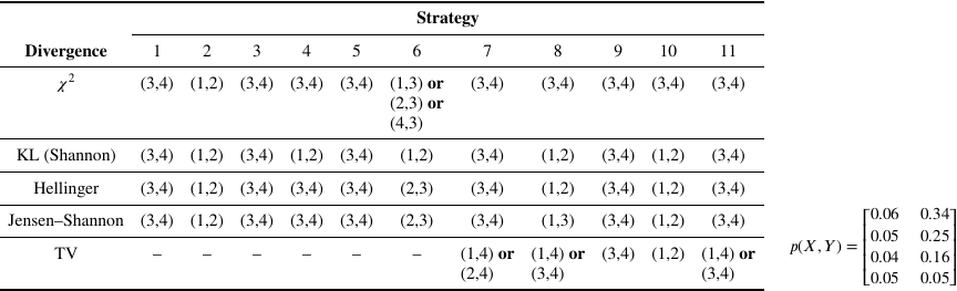
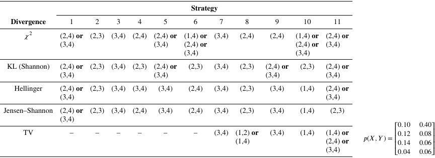
Table 3 summarizes the strategies considered for simplifying \(X\) using four \(E^{\mathit{Top}}_{f}(p)\) entropies (\(\chi^2\), Hellinger, Shannon, and Jensen–Shannon) and five \(J^{C{\&}A}_{f}(p)\) negentropies (\(\chi^2\), Hellinger, Shannon, Jensen–Shannon, and TV). The resulting optimal groupings for two toy examples are reported in Tables 4 and 5.
For Shannon entropy, several strategies are algebraically equivalent, namely Strategies 2, 4, 6, and 10; Strategies 3 and 7; and Strategies 1, 5, and 9, leading to identical objective functions and outcomes. Apart from the trivial behavior of Strategy 1, which always groups the two smallest marginal symbols of \(X\) by construction, the optimal grouping generally depends on both the chosen strategy and the divergence or negentropy. This dependence is expected, as the strategies encode distinct information-theoretic trade-offs.
The remarkable stability of Strategy 2, which minimizes \(I_{f}(X;Y) - I_{f}(X';Y)\), across different divergences can be explained by the local equivalence of \(f\)-divergences. In particular, any \(f\)-divergence admits a second-order approximation by a \(\chi^2\)-divergence around the reference distribution 32. Since all candidate groupings in the toy examples correspond to small perturbations, different divergences induce nearly identical rankings, yielding the same optimal grouping. Strategies 1–6 exhibit a high degree of robustness across divergences, with optimal groupings largely determined by marginal weights and similarity of conditional distributions.
A particularly strong regularity in the examples in Tables 4 and 5 concerns the Hellinger and Jensen–Shannon divergences. Both divergences are symmetric, bounded, and primarily sensitive to distributional overlap rather than tail behavior. In our examples, for most candidate groupings, the induced changes in the joint distribution are relatively small and clearly ordered, so that both divergences rank them in the same way. Differences only emerge when two or more groupings produce very similar levels of information loss. The example in Table 6 is constructed precisely in this near-tie regime, where these differences lead to distinct optimal groupings.

| Strategy 11 | |||
| Divergence | \(\lambda=0\) | \(\lambda=1\) | \(\lambda=2\) |
| \(\chi^2\) | (3,4) | (3,4) | (3,4) |
| KL (Shannon) | (3,4) | (3,4) | (3,4) |
| Hellinger | (3,4) | (3,4) | (3,4) |
| Jensen–Shannon | (3,4) | (3,4) | (3,4) |
| TV | (3,4) | (1,4) or (3,4) | (1,4) |
Strategies 7–11, based on Cichocki–Amari negentropies, introduce an additional modeling choice by explicitly penalizing the removal of zero-probability symbols following grouping. In the reported results, we fix \(\lambda=1\); varying \(\lambda\) changes the balance between grouping distortion and symbol elimination and may therefore alter the selected grouping. To provide a minimal illustration of the role of the regularization parameter \(\lambda\), Table 7 reports the sensitivity of Strategy 11 in Toy Example 1 for \(\lambda \in \{0, 1, 2\}\). The optimal merge is stable for KL, \(\chi^2\), Hellinger, and Jensen–Shannon, whereas TV negentropy changes its recommended merge as \(\lambda\) grows. For KL this can be understood analytically: the zero-removal penalty reduces to \(\log(n/(n-1))\), a constant independent of the merge, so \(\lambda\) has no effect on the ranking. For the remaining divergences, no such analytical guarantee exists.
Behavior on Sparse and Heavy-Tailed Distributions
The toy examples above use short, roughly balanced distributions. To illustrate the qualitative behavior of the framework in a sparser regime, consider a Zipf-distributed marginal with \(n=6\) symbols and exponent \({s=1}\): \({p_{k} \propto 1/k}\), giving approximately \(p = (0.408, 0.204, 0.136, 0.102, 0.082, 0.068)\). This distribution is far from uniform, with the largest symbol holding roughly six times the mass of the smallest.
In the marginal-only setting (Strategy 1, grouping the two smallest), the selected merge is always \((5,6)\) regardless of the divergence, since this is determined purely by rank order. However, when a joint distribution couples \(X\) to a response variable \(Y\) (for instance a binary label), the preferred merge under Strategies 2–6 will depend on how the conditional distributions \(p(Y|x_{k})\) vary with \(k\). For Zipf-like marginals, the dominant symbol \(x_1\) carries the largest marginal weight; if the joint distribution also concentrates discriminative information on \(x_1\), merging it with any other symbol causes a large drop in \(f\)-information, which is correctly penalized by all joint-distribution strategies. Meanwhile, the tail symbols \(x_5\) and \(x_6\) carry little mass, so merging them causes little distortion under most strategies.
This behavior generalizes: in sparse or heavy-tailed regimes, the local \(\chi^2\) approximation underlying the near-equivalence of \(f\)-divergences 32 breaks down when the dominant symbol has a much larger mass than the merged pair. In such cases, heavy-tail-sensitive divergences such as \(\chi^2\) can recommend different merges from less tail-sensitive ones such as Hellinger, and the choice of divergence becomes more consequential. A systematic study of this phenomenon—including comparisons on softmax outputs from classifiers trained on standard benchmarks—is a natural direction for future work.
9. Conclusions and Future Work
In this paper, we extended the framework introduced in 9,17 of generalized entropies derived from \(f\)-divergences to guide the dimensionality reduction of finite distributions. Majorization relations between candidate groupings provide a divergence-independent baseline for simplification, since the induced order is reversed for all such entropies.
When dimensionality reduction must preserve a joint distribution, we analyzed the analogy with Shannon’s information channel and proved that, among all entropies and negentropies derived from \(f\)-divergences in both the Topsøe and Cichocki–Amari frameworks, Shannon entropy (and its associated negentropy) is the only one that satisfies the classical channel equations.
Although the exact channel identities hold exclusively for Shannon entropy, alternative objective functions can still guide simplification. For Topsøe entropies, invariance under zero-probability symbol removal ensures that entropy- and information-based criteria remain well defined. In contrast, Cichocki–Amari entropies depend explicitly on the alphabet size and cannot be used directly for dimensionality reduction. To address this limitation, we adopted the corresponding negentropies and introduced regularized negentropy-based strategies that remain consistent under grouping and zero removal.
Future work includes studying higher-dimensional or sparse regimes, where different objective functions may lead to qualitatively distinct simplifications, as well as a more systematic comparison and combination of simplification strategies. The framework is also naturally applicable to the post-hoc simplification of high-dimensional probability distributions. These distributions naturally arise when discrete variables have large alphabets, such as softmax outputs in classification or token distributions in language models, and become especially relevant when such representations are coupled to other variables through a joint distribution. Finally, developing efficient search strategies for \(I_f\)-based merge criteria—analogous to the incremental updates available for Shannon mutual information—remains an important open problem.
Acknowledgments
This work has been supported by grant PID2023-149976OB-C22 funded by MICIU/AEI/10.13039/501100011033 and by ERDF/EU. The authors acknowledge the use of AI-based language models (ChatGPT versions 5.1 and 5.2) for assistance with the computation and verification of the results reported in Tables 4–6, for support in reorganizing and checking mathematical proofs, and for help with LaTeX troubleshooting and manuscript preparation. Claude (Anthropic) was additionally used for assistance with the preparation of the revised manuscript, including LaTeX editing and manuscript revision. All scientific content and interpretations remain the sole responsibility of the authors.
- [1] A. Krizhevsky, I. Sutskever, and G. E. Hinton, “ImageNet classification with deep convolutional neural networks,” Proc. 26th Int. Conf. Neural Inf. Process. Syst. (NIPS), Vol.1, pp. 1097-1105, 2012.
- [2] T. B. Brown et al., “Language models are few-shot learners,” arXiv:2005.14165, 2020. https://doi.org/10.48550/arXiv.2005.14165
- [3] F. A. Cowell, “Measuring Inequality (3rd Edition),” Oxford University Press, 2011.
- [4] L. Martino, V. Elvira, and F. Louzada, “Effective sample size for importance sampling based on discrepancy measures,” Signal Process., Vol.131, pp. 386-401, 2017. https://doi.org/10.1016/j.sigpro.2016.08.025
- [5] T. Leinster and C. A. Cobbold, “Measuring diversity: The importance of species similarity,” Ecology, Vol.93, No.3, pp. 477-489, 2012. https://doi.org/10.1890/10-2402.1
- [6] A. Rényi, “On measures of entropy and information,” Proc. 4th Berkeley Symp. Math. Stat. Probab., Vol.1, pp. 547-561, 1961.
- [7] C. Tsallis, “Possible generalization of Boltzmann-Gibbs statistics,” J. Stat. Phys., Vol.52, No.1, pp. 479-487, 1988. https://doi.org/10.1007/BF01016429
- [8] T. M. Cover and J. A. Thomas, “Elements of Information Theory,” John Wiley & Sons, 2006.
- [9] M. Sbert, M. Chen, J. Poch, M. Feixas, and S. Chen, “Entropies from f-divergences,” Proc. 21st Int. Conf. Model. Decis. Artif. Intell. (MDAI 2024), pp. 47-60, 2024. https://doi.org/10.1007/978-3-031-68208-7_5
- [10] G. Hardy, J. Littlewood, and G. Pólya, “Inequalities,” 2nd Edition, Cambridge University Press, 1952.
- [11] A. W. Marshall, I. Olkin, and B. C. Arnold, “Inequalities: Theory of Majorization and Its Applications,” 2nd Edition, Springer, 2011. https://doi.org/10.1007/978-0-387-68276-1
- [12] B. C. Arnold, “Majorization and the Lorenz Order: A Brief Introduction,” Springer, 1987. https://doi.org/10.1007/978-1-4615-7379-1
- [13] P. Castelló, M. Sbert, M. Chover, and M. Feixas, “Viewpoint-based simplification using -divergences,” Inf. Sci., Vol.178, No.11, pp. 2375-2388, 2008. https://doi.org/10.1016/j.ins.2008.01.011
- [14] J. Rigau, M. Feixas, and M. Sbert, “Refinement criteria based on -divergences,” Proc. 14th Eurogr. Workshop Render., pp. 260-269, 2003.
- [15] M. Feixas and M. Sbert, “The role of the information channel in visual computing,” M. Chen, J. M. Dunn, A. Golan, and A. Ullah (Eds.), “Advances in Info-Metrics: Information and Information Processing Across Disciplines,” pp. 464-490, Oxford University Press, 2020. https://doi.org/10.1093/oso/9780190636685.003.0017
- [16] M. Sbert, M. Feixas, J. Rigau, M. Chover, and I. Viola, “Information Theory Tools for Computer Graphics,” Springer, 2023. https://doi.org/10.1007/978-3-031-79546-6
- [17] M. Sbert, M. Chen, J. Poch, M. Feixas, S. Chen, and V. Elvira, “Dimensionality reduction with entropies from f-divergences,” Proc. 22nd Int. Conf. Model. Decis. Artif. Intell. (MDAI), pp. 27-41, 2026. https://doi.org/10.1007/978-3-032-00891-6_3
- [18] I. Csiszár and P. C. Shields, “Information theory and statistics: A tutorial,” Found. Trends Commun. Inf. Theory, Vol.1, No.4, pp. 417-528, 2004. https://doi.org/10.1561/0100000004
- [19] I. Sason, “On data-processing and majorization inequalities for -divergences with applications,” Entropy, Vol.21, No.10, Article No.1022, 2019. https://doi.org/10.3390/e21101022
- [20] Y. Polyanskiy and Y. Wu, “Information Theory: From Coding to Learning,” Cambridge University Press, 2025. https://doi.org/10.1017/9781108966351
- [21] A. Cichocki and S. Amari, “Families of Alpha- Beta- and Gamma-divergences: Flexible and robust measures of similarities,” Entropy, Vol.12, No.6, pp. 1532-1568, 2010. https://doi.org/10.3390/e12061532
- [22] F. Topsøe, “Entropy and equilibrium via games of complexity,” Phys. A Stat. Mech. Appl., Vol.340, Nos.1-3, pp. 11-31, 2004. https://doi.org/10.1016/j.physa.2004.03.073
- [23] O. Rioul, “The interplay between error, total variation, alpha-entropy and guessing: Fano and Pinsker direct and reverse inequalities,” Entropy, Vol.25, No.7, Article No.978, 2023. https://doi.org/10.3390/e25070978
- [24] J.-J. Egozcue and V. Pawlowsky-Glahn, “Evidence functions: A compositional approach to information,” SORT-Stat. Oper. Res. Trans., Vol.42, No.2, pp. 101-124, 2018.
- [25] J. Aczél and Z. Daróczy, “On Measures of Information and Their Characterizations,” Academic Press, 1975.
- [26] F. Cowell, “Measuring Inequality,” Oxford University Press, 2011. https://doi.org/10.1093/acprof:osobl/9780199594030.001.0001
- [27] C. E. Shannon, “A mathematical theory of communication,” Bell Syst. Tech. J., Vol.27, No.3, pp. 379-423 and Vol.27, No.4, pp. 623-656, 1948. https://doi.org/10.1002/j.1538-7305.1948.tb01338.x, https://doi.org/10.1002/j.1538-7305.1948.tb00917.x
- [28] T. W. Chaundy and J. B. McLeod, “On a functional equation,” Edinb. Math. Notes, Vol.43, pp. 7-8, 1960. https://doi.org/10.1017/S0950184300003244
- [29] N. Slonim and N. Tishby, “Agglomerative information bottleneck,” Proc. 13th Int. Conf. Neural Inf. Process. Syst. (NIPS’99), pp. 617-623, 1999.
- [30] A. Bardera, J. Rigau, I. Boada, M. Feixas, and M. Sbert, “Image segmentation using information bottleneck method,” IEEE Trans. Image Process., Vol.18, No.7, pp. 1601-1612, 2009. https://doi.org/10.1109/TIP.2009.2017823
- [31] M. Sato, “Presentation of a new formulation of negentropy: 1st report, basic concepts,” Bull. JSME, Vol.25, No.202, pp. 599-605, 1982. https://doi.org/10.1299/JSME1958.25.599
- [32] F. Nielsen and R. Nock, “On the chi square and higher-order chi distances for approximating -divergences,” IEEE Signal Process. Lett., Vol.21, No.1, pp. 10-13, 2014. https://doi.org/10.1109/LSP.2013.2288355
Appendix
Appendix A. Solution of \(g(nx) - g(n(1-x)) = g(x) - g(1-x)\)
We solve the functional equation for \(g\):
Proposition 16 (Uniqueness under smoothness). Let \(f\colon {(0,\infty) \to \mathbb{R}}\) be convex and twice continuously differentiable, with
Proof. Fix \(x \in (0,1)\). For each \(n>0\), define
Integrating from 1 to \(x\), we obtain
Since \(g=f'\), we integrate once more:
From \(f(0^{+})=0\), we must have \(\alpha - \beta =0\) (the term \(x\log x\) tends to \(0\) as \(x\to 0^{+}\)). Thus \(\beta=\alpha\). Therefore,
Finally, convexity of \(f\) gives
Appendix B. Derivation of the Fundamental Equation of Information
Consider a three-element partition
Let \(f \colon {[0,1] \to \mathbb{R}}\) be any function and define the entropy of a binary distribution \((p, 1-p)\) by
B.1. Conditional Entropy of \(Y\) Given \(X\)
Consider, for \({x+y} \le 1\), conditional distributions of \(Y\) given \(X\)
Thus,
B.2. Conditional Entropy of \(X\) Given \(Y\)
The conditional distributions of \(X\) given \(Y\) are
Hence,
B.3. Fundamental Equation of Information
The identity
B.4. Normalization \(f(0)=f(1)=0\)
Under the common conditions \(f(0)=f(1)=0\), this reduces to
This is the fundamental equation of information 25 expressed entirely in terms of the binary entropy generator \(f\), and has as only solution \(f(x)= cx \log x\), \(c \ge 0\).
Appendix C. Multiplicative Cauchy Equation and Shannon Generator
Proposition 17. Let \(f \colon {(0,\infty) \to \mathbb{R}}\) be convex and satisfy \(f(1)=0\). Assume that for all \(x,y>0\),
Proof. Define \(g \colon {(0, \infty) \to \mathbb{R}}\) by \(g(x) := f(x)/x\). Then Eq. (39) is equivalent to the multiplicative Cauchy equation
Because \(f\) is convex on \((0,\infty)\), it is continuous and therefore bounded on every compact interval. Consequently \(g\) is bounded on compact subsets of \((0,\infty)\), and \(h\) is locally bounded on \(\mathbb{R}\). By the classical regularity theorem for Cauchy’s functional equation, any locally bounded solution of Eq. (42) must be linear 25. Hence, there exists \({c \in \mathbb{R}}\) such that \({h(t) = ct}\) for all \({t \in \mathbb{R}}\).
Therefore \(g(x)=c\log x\) for all \(x>0\), and thus \(f(x)=xg(x)=c\,x\log x\). The convexity of \(f\) implies \(c\ge 0\), since \((c\,x\log x)''=c/x\ge 0\). Finally, \(\lim_{x\rightarrow 0}c\,x\log x=0\), so \(f(0)=0\) under the natural extension. ∎
Appendix D. C&A Negentropy: Direct Derivation of the FEI
This appendix mirrors Appendix B in the Cichocki–Amari negentropy setting.
Consider a three-element partition
Let \(f \colon {(0,\infty) \to \mathbb{R}}\) be convex with \(f(1) = f(0) = 0\). For a binary distribution \((p, 1-p)\) where \(u_{2} = (1/2, 1/2)\),
D.1. Conditional C&A Negentropy
Define conditional negentropy by averaging conditional negentropies:
For \(x+y<1\), the conditional distributions are
D.2. Negentropy Channel Identity
Assume that the negentropy identity holds:
Using Eq. (43), note first that
Therefore,
Substitute Eqs. (45) and (46) into Eq. (44) and multiply by 2. We obtain
D.3. Reduction to the FEI
Introduce the rescaled and normalized generator
Since \(f\) is convex, \(\psi\) is convex and therefore continuous on \([0,1]\). Under the normalization \(\psi(0) = \psi(1) = 0\), the fundamental equation of information has the solution
This article is published under a Creative Commons Attribution-NoDerivatives 4.0 Internationa License.