
Research Paper:
Data-Driven Portfolio Optimization Using a Predict-Then-Optimize Framework
Yi Wang†
 and Takashi Hasuike
Graduate School of Science and Engineering, Waseda University
3-4-1 Okubo, Shinjuku-ku, Tokyo 169-8555, Japan
†Corresponding author

Effective portfolio diversification remains a central challenge in quantitative asset management. In this study, we propose a data-driven framework based on the predict-then-optimize (PO) paradigm, which combines return forecasting with portfolio allocation in a sequential manner. The forecasting module employs DLinear, a lightweight deep learning model, to capture temporal patterns in historical asset returns. Based on the predicted returns, a portfolio allocation strategy is constructed by optimizing the Sharpe ratio, allowing the model to generate adaptive portfolio weights under changing market conditions. This PO-based framework provides a practical way to connect predictive modeling with downstream decision-making. Empirical results across three asset universes demonstrate that the proposed approach achieves competitive performance under different settings, indicating its potential applicability in real-world portfolio management.
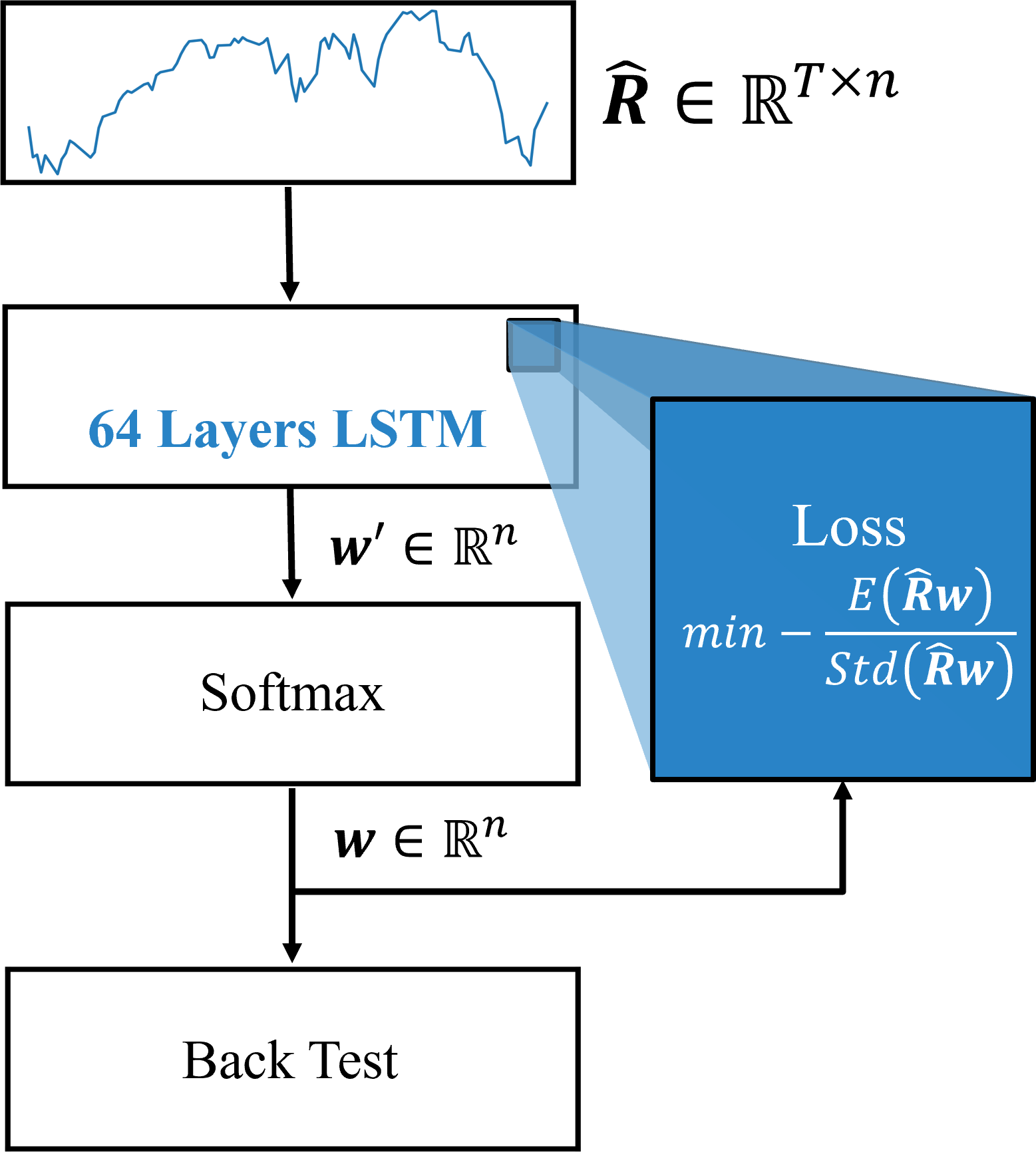
The neural network in allocation step
1. Introduction
1.1. Background
1.1.1. Deep Learning Approaches to the Portfolio Optimization Problem
Portfolio optimization is a fundamental tool in investment management, aiming to determine the optimal asset allocation. The goal is to maximize returns under a fixed level of risk or to minimize risk while ensuring returns exceed a specified threshold.
With the rapid advancement of deep learning technologies, their applications in the financial domain have grown substantially. Deep learning’s strengths in pattern recognition and nonlinear modeling—demonstrated in fields such as image recognition and natural language processing—allow it to better capture the complex dynamics and interdependencies inherent in financial markets.
These capabilities not only improve the efficiency of portfolio construction but also help mitigate investment risks and support more stable decision-making under market uncertainty.
1.1.2. Developments in the Portfolio Optimization Problem
The theory of portfolio optimization was pioneered by Markowitz in his seminal work, which introduced the well-known mean-variance (MV) model 1. One of the key advantages of portfolio construction using the MV model is its ability to enhance returns while diversifying risk, compared to investing in individual assets.
Following the introduction of the MV model by Markowitz, Sharpe proposed the Sharpe ratio (SR) 2 as a modern modeling approach in portfolio optimization. The SR evaluates not only the return of an asset but also its associated risk, measuring risk-adjusted returns and indicating the price of risk per unit. Because it comprehensively reflects the risk-return characteristics of capital markets, the SR is widely used for assessing portfolio performance, evaluating market efficiency, constructing effective portfolios, and supporting investment decision-making.
Furthermore, based on Markowitz’s theory and equilibrium concepts, Sharpe proposed the capital asset pricing model 3, which has been extensively applied in areas such as asset valuation and budgeting of capital costs.
Subsequently, Black and Litterman 4 proposed the Black–Litterman model, which combines investors’ subjective views with historical market data. In this model, the market distribution is treated as the prior distribution and the investor’s views as the conditional distribution. By combining these two, the model derives a posterior distribution used for portfolio optimization.
In recent years, the advancement of computational power has driven significant progress in portfolio optimization theory through the development of more diverse formulations, solution methods, and nonlinear modeling capabilities. Techniques such as stochastic optimization 5, time series analysis 6,7, deep learning 8,9,10, and reinforcement learning 11,12 have become widely adopted in this domain.
1.1.3. Challenges in Applying Deep Learning to the Investment Domain
It is undeniable that the ability to accurately predict future asset prices would be highly beneficial for making future investment decisions. Investors have attempted such predictions using models such as autoregressive integrated moving average, generalized autoregressive conditional heteroskedasticity, machine learning models 13, and deep learning models 14. However, due to the Brownian motion-like behavior of asset price movements, forecasting asset prices remains an extremely difficult task. Therefore, selecting appropriate input features—among various available indicators such as prices, price-to-earnings ratio (PER), and price-to-book ratio (PBR)—as well as choosing the right prediction model is crucial for achieving accurate asset price forecasts.
In addition, most existing deep learning models primarily focus on the prediction step. When it comes to asset allocation within a given universe, traditional models or equally weighted investment strategies are often used, with little consideration given to the post-prediction allocation process. Expanding the solution space of portfolio optimization using deep learning remains a promising direction for future research.
1.2. Research Objectives
This study aims to develop a portfolio optimization algorithm that leverages deep learning models to generate optimal investment decisions based on predicted asset returns.
1.3. Organization of the Paper
This paper consists of the following six sections. Section 1 presents the background and objectives of the study, as well as the overall structure of the paper. In the subsequent sections, key terminology is also introduced. Section 2 reviews several prior studies that are relevant to this research. Section 3 describes the architecture of the deep learning model proposed in this study and explains how its intended functions are realized. Section 4 outlines the types of datasets used, the methodology for evaluating the algorithm’s performance, and the experimental environment. Section 5 presents the experimental results and their analysis. It compares outcomes under different experimental conditions and discusses the effectiveness of the proposed method. Section 6 provides the final conclusions of the study and discusses potential directions for future research.
1.4. Evaluation Metrics for Prediction
-
1.
Mean absolute error (MAE) measures the average absolute difference between predicted and actual values. It is calculated by summing the absolute errors of each data point and taking the average. The formula is as follows:
\begin{equation} \text{MAE} = \frac{1}{n} \sum_{i=1}^{n} \left| y_i - \hat{y}_i \right| . \tag{1} \end{equation} -
2.
Mean absolute percentage error (MAPE) measures the average percentage difference between predicted and actual values. The formula is as follows:
\begin{equation} \text{MAPE} = \frac{1}{n} \sum_{i=1}^{n} \left| \frac{y_i - \hat{y}_i}{y_i} \right| \times 100\% . \tag{2} \end{equation} -
3.
Mean squared error (MSE) measures the average of the squared differences between predicted and actual values. The formula is given by:
\begin{equation} \text{MSE} = \frac{1}{n} \sum_{i=1}^{n} \left( y_i - \hat{y}_i \right)^2 . \tag{3} \end{equation} -
4.
Root mean squared error (RMSE) is the square root of the MSE and provides the error in the same unit as the original data. It is computed as:
\begin{equation} \text{RMSE} = \sqrt{ \frac{1}{n} \sum_{i=1}^{n} \left( y_i - \hat{y}_i \right)^2 } . \tag{4} \end{equation}
3. Proposed Method
This section describes the proposed investment method, which consists of two main components: forecasting future returns based on historical return data, and modeling both return and risk in order to generate an optimal portfolio allocation.
3.1. Discussion on Conventional Methods
The method proposed by Zhang et al. 10 aims to optimize the SR in order to obtain an investment portfolio. Specifically, they input eight features—date, open, high, low, close, adjusted close, volume, and return—into a 64-layer long short-term memory (LSTM) 21 network. The loss function is defined as the SR, and the output vector is passed through a SoftMax function to obtain a portfolio allocation vector whose elements sum to one. Investments are executed based on this vector. During the backtest period, the model receives the most recent 50 days of data at the beginning of each month, outputs portfolio weights for that month, and repeats this process monthly.
Although their method directly utilizes a neural network to generate portfolio weights, it still inherits a key limitation of the MV model—namely, it uses historical returns directly as a proxy for future expected returns. Given that deep learning-based time series forecasting has been widely validated for its effectiveness, we consider a framework in which a deep learning model is first used to forecast future returns, and these predicted returns are then fed into an LSTM model to generate the final portfolio allocation.
3.2. Preliminary Evaluation of the Proposed Method
To evaluate the validity of our idea, we conducted a simple empirical test using data from January 1, 2021 to January 1, 2022. We focused on three assets: SPY, VTI, and JPXN. For each asset, we employed the DLinear model (Figs. 1 and 2) to forecast the average return for the upcoming month at the beginning of each month, using the most recent 50 days of data up to that point.
We then compared the predicted monthly returns with the actual values and computed the following evaluation metrics: MAE, MAPE, MSE, and RMSE. The results are summarized in Tables 1 and 2.
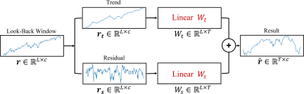
Fig. 1. Time series decomposition in the prediction model.
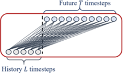
Fig. 2. Mechanism of DLinear.
| Ticker | MAE | MAPE | MSE | RMSE |
| SPY | 0.035257 | 2.443033 | 0.001842 | 0.042916 |
| VTI | 0.034432 | 2.349176 | 0.001742 | 0.041739 |
| JPXN | 0.027523 | 2.256462 | 0.001232 | 0.035104 |
| Ticker | MAE | MAPE | MSE | RMSE |
| SPY | 0.034517 | 2.331798 | 0.001480 | 0.038468 |
| VTI | 0.023594 | 1.577607 | 0.000811 | 0.028485 |
| JPXN | 0.044399 | 3.688388 | 0.002372 | 0.048705 |
From the tables above, it can be observed that DLinear yields better forecasting performance for SPY and VTI, while for JPXN, using the simple average of the most recent 50 days appears to provide more reliable results. Overall, the predictive approach based on DLinear demonstrates effectiveness and can be considered a meaningful improvement.
3.3. Proposed Deep Learning Model
The model proposed in this study is divided into two components: a prediction step and an allocation step.
3.3.1. Prediction Step
The decomposition of the original input time series into trend and residual components in the model is expressed by the following equations:
Here, \(L = 48\) denotes the length of the look-back window, and \(T = 24\) is the length of the forecasting window. The constant \(c = 1\) indicates that a single feature (return) is used for both training and inference. The model is optimized using the Adam optimizer.
To simulate real investment behavior, multi-step forecasts are performed on a monthly basis with a step size of 24 over the period from January 2021 to January 2022. The predicted monthly returns are subsequently used as input to the allocation model. Furthermore, before predicting each monthly return, the model is trained on a rolling window of one year.
3.3.2. Allocation Step
In the allocation step, we adopt a 64-layer LSTM model as the neural network architecture (Fig. 3). The predicted returns from the prediction step are fed into the network, which outputs a vector \(w' \in \mathbb{R}^n\). The magnitude of each element in this vector represents the relative preference for investing in each of the \(n\) assets.
However, since the sum of the values in \(w'\) does not necessarily equal 1, it cannot be directly used as a valid portfolio allocation. To address this, the vector is passed through a SoftMax function to obtain the final portfolio weight vector \(w \in \mathbb{R}^n\), which satisfies the constraint that all elements sum to one.
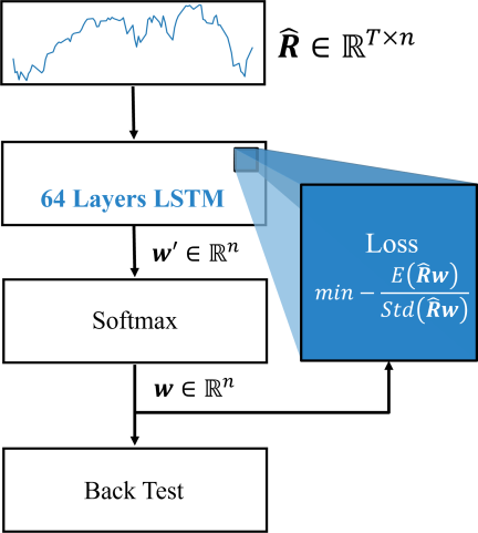
Fig. 3. The neural network in allocation step.
For the loss function, we adopt the SR. Specifically, the predicted return matrix \(\hat{R}\) is multiplied by the weight vector \(w\) to obtain the predicted portfolio return for the corresponding month. The mean and standard deviation of the resulting return vector are then calculated, and the SR is maximized by minimizing its negative value as the loss function.
4. Experimental Overview
4.1. Experimental Environment
The basic experimental environment used in this study is summarized in Table 3.
| Component | Specification |
| Operating system | Windows 10 64-bit |
| CPU | 12th Gen Intel Core i5-12400F (12 CPUs), 2.5 GHz, 32.0 GB RAM |
| GPU | NVIDIA GeForce RTX 4060 Ti |
| VRAM | Dedicated memory: 7964 MB |
| Programming language | Python 3.9.18 |
| Data source | yfinance |
| ML library | scikit-learn 1.3.2 |
| DL libraries | PyTorch 1.8.2, TensorFlow 2.15.0 |
| Optimization library | SciPy 1.11.4 |
4.2. Experimental Design
The experiment in this study consists of three steps: prediction, allocation, and backtesting. In the prediction step, the DLinear model is used to generate return forecasts. These forecasts are then passed to an LSTM model to obtain the portfolio weights. Using these weights, a financial investment simulation is conducted within a selected asset universe. This simulation process is referred to as backtesting.
The method of sliding the time window in the prediction step is illustrated in Fig. 4.
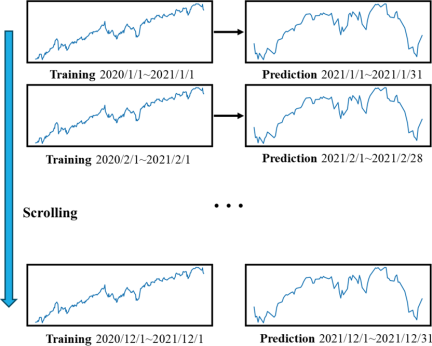
Fig. 4. Time-series rolling window design.
4.3. Dataset Description and Backtest Framework
The backtesting strategy involves generating forecasts using deep learning models and allocating the portfolio based on the predicted returns at the beginning of each period during the backtesting window from January 1, 2021 to January 1, 2022. To examine the robustness of the proposed method across different market regimes, we additionally conduct a long-horizon backtest over the period 2018–2022 for Universe 1, which covers diverse market conditions, including bull markets, volatile periods, and extreme shocks such as the COVID-19 crisis.
4.3.1. Universe 1
We first evaluate the proposed model using a selected universe, referred to as Universe 1. This universe consists of eight major MSCI iShares ETFs representing a broad spectrum of markets, including equities, bonds, and commodities.
The eight ETFs in Universe 1 are as follows:
-
・
SPDR S&P 500 ETF Trust (SPY)
-
・
iShares MSCI EAFE ETF (EFA)
-
・
iShares MSCI Emerging Markets ETF (EEM)
-
・
iShares JPX-Nikkei 400 ETF (JPXN)
-
・
Technology Select Sector SPDR Fund (XLK)
-
・
iShares Core U.S. Aggregate Bond ETF (AGG)
-
・
Invesco DB Commodity Index Tracking Fund (DBC)
-
・
Vanguard Total Stock Market ETF (VTI)
For benchmarking purposes, we compare the backtest results of Universe 1 against three strategies: an equally weighted portfolio, the SPY index, and the classical MV model. To simulate realistic investment behavior, we also conduct backtest using the Backtrader library.
4.3.2. Universe 2
To evaluate the generalizability and robustness of the proposed algorithm, we conducted a backtest using a second universe composed of 20 ETFs randomly selected from the MSCI ETF pool.
The selected ETFs are as follows: IAI, IVV, ESGU, QUAL, SLV, IWB, HEWJ, RING, IAU, IYY, EWT, ITOT, IWV, IAK, ILCB, DIVB, ICVT, DGRO, IFRA, and PICK.
4.3.3. Universe 3
In the previous two universes, we observed that assets with poor performance were occasionally assigned near-zero weights. This suggests that the model possesses a certain level of discriminative capability. Therefore, we aim to further investigate whether the model can be used for asset selection.
To verify this aspect, we constructed a third universe consisting of all MSCI ETFs issued before 2015. The model was applied to perform both prediction and allocation, followed by backtesting. A full list of all ETFs used in Universe 3 is available upon request.
4.4. Experimental Settings
| Component | Hyperparameter | Value |
| Prediction model (DLinear) | ||
| Number of epochs | 200 | |
| Batch size | 64 | |
| Learning rate | \(1 \times 10^{-4}\) | |
| Input sequence length (\(seq\_len\)) | 48 | |
| Prediction horizon (\(pred\_len\)) | 24 | |
| Moving average window (kernel size) | 21 | |
| Optimizer | Adam | |
| Allocation model (LSTM-based) | ||
| LSTM hidden units | 64 | |
| Output activation | Softmax | |
| Optimizer | Adam | |
| Number of epochs | 20 | |
Table 4 summarizes the hyperparameter settings for both the prediction and allocation models.
5. Experimental Results and Discussion
5.1. Results of the Prediction Step
The deep learning model used in the prediction step is DLinear. For comparison, we also implemented a forecasting model using XGBoost under the same rolling window scheme. The prediction performance was evaluated using four comprehensive metrics: MAE, MAPE, MSE, and RMSE.
The results of the prediction step for Universes 1 and 2 are summarized in Tables 5–8 and Fig. 5.
| Ticker | MAE | MAPE | MSE | RMSE |
| AGG | 0.0148 | 1.456 | 0.00030 | 0.0173 |
| DBC | 0.0764 | 6.279 | 0.00726 | 0.0852 |
| EEM | 0.1012 | 7.856 | 0.01082 | 0.1040 |
| EFA | 0.0329 | 2.723 | 0.00131 | 0.0362 |
| JPXN | 0.0444 | 3.688 | 0.00237 | 0.0487 |
| SPY | 0.0345 | 2.332 | 0.00148 | 0.0385 |
| VTI | 0.0236 | 1.578 | 0.00081 | 0.0285 |
| XLK | 0.0869 | 4.433 | 0.01122 | 0.1059 |
| Ticker | MAE | MAPE | MSE | RMSE |
| AGG | 0.0164 | 1.624 | 0.00035 | 0.0188 |
| DBC | 0.3794 | 29.634 | 0.15918 | 0.3990 |
| EEM | 0.2483 | 18.973 | 0.06479 | 0.2545 |
| EFA | 0.2354 | 19.291 | 0.05656 | 0.2378 |
| JPXN | 0.1958 | 16.151 | 0.03928 | 0.1982 |
| SPY | 0.3668 | 24.765 | 0.14453 | 0.3802 |
| VTI | 0.3944 | 26.223 | 0.16358 | 0.4045 |
| XLK | 0.5539 | 29.087 | 0.33653 | 0.5801 |
| Ticker | MAE | MAPE | MSE | RMSE |
| DGRO | 0.0315 | 2.402 | 0.00138 | 0.0371 |
| DIVB | 0.0387 | 2.818 | 0.00201 | 0.0449 |
| ESGU | 0.0360 | 2.405 | 0.00192 | 0.0438 |
| EWT | 0.0546 | 3.246 | 0.00484 | 0.0696 |
| HEWJ | 0.0269 | 2.142 | 0.00133 | 0.0364 |
| IAI | 0.0665 | 4.229 | 0.00597 | 0.0773 |
| IAK | 0.0378 | 3.419 | 0.00182 | 0.0427 |
| IAU | 0.0242 | 2.006 | 0.00109 | 0.0330 |
| ICVT | 0.0716 | 4.299 | 0.00937 | 0.0968 |
| IFRA | 0.0403 | 3.160 | 0.00236 | 0.0485 |
| ILCB | 0.0321 | 2.213 | 0.00163 | 0.0403 |
| ITOT | 0.0341 | 2.332 | 0.00175 | 0.0419 |
| IVV | 0.0355 | 2.466 | 0.00184 | 0.0429 |
| IWB | 0.0344 | 2.348 | 0.00177 | 0.0421 |
| IWV | 0.0340 | 2.328 | 0.00174 | 0.0416 |
| Ticker | MAE | MAPE | MSE | RMSE |
| IAI | 0.6150 | 36.863 | 0.3995 | 0.6320 |
| IVV | 0.3666 | 24.791 | 0.1444 | 0.3800 |
| ESGU | 0.3966 | 25.827 | 0.1670 | 0.4087 |
| PICK | 0.6553 | 39.244 | 0.4407 | 0.6639 |
| QUAL | 0.3511 | 23.893 | 0.1338 | 0.3658 |
| SLV | 0.2505 | 17.024 | 0.0733 | 0.2708 |
| IWB | 0.3858 | 25.689 | 0.1577 | 0.3971 |
| HEWJ | 0.2494 | 19.767 | 0.0638 | 0.2527 |
| RING | 0.0848 | 6.701 | 0.0106 | 0.1030 |
| IAU | 0.0276 | 2.253 | 0.00132 | 0.0363 |
| IYY | 0.3841 | 25.701 | 0.1564 | 0.3954 |
| EWT | 0.5575 | 32.421 | 0.3176 | 0.5636 |
| ITOT | 0.3924 | 26.166 | 0.1619 | 0.4024 |
| IWV | 0.3917 | 26.111 | 0.1614 | 0.4018 |
| IAK | 0.2661 | 23.668 | 0.0756 | 0.2750 |
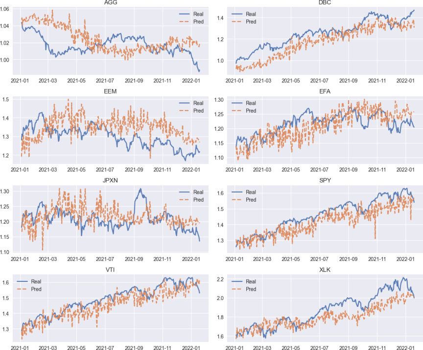
Fig. 5. Prediction results of DLinear model. The yellow line represents the predicted values, while the blue line indicates the actual observed values. The DLinear model demonstrates strong predictive performance for assets exhibiting clear trend characteristics. However, in cases where the asset exhibits repetitive fluctuations or lacks regularity, the model struggles to capture the underlying patterns, resulting in lower prediction accuracy.
As shown in the tables, DLinear outperforms XGBoost across all four evaluation metrics. In particular, XGBoost appears to suffer from underfitting on the dataset used in this study. This is likely due to the lack of a time-series decomposition mechanism in XGBoost, which makes it less effective at capturing temporal structures inherent in financial return data.
5.2. Backtest Result
As shown in Table 9, the turnover levels remain moderate across all asset universes.
| Asset universe | Average turnover |
| U1 (8 assets) | 0.1030 |
| U2 (20 assets) | 0.3452 |
| U3 (Full set) | 0.2712 |
5.2.1. Result of Universe 1
The blue line represents the backtest performance of the proposed algorithm, the orange line corresponds to SPY, the green line to the equally weighted strategy, and the red line to the MV model (Figs. 6 and 7). These results indicate that the two-stage deep learning-based prediction and allocation strategy delivers higher returns than SPY, the equally weighted approach, and the MV model.
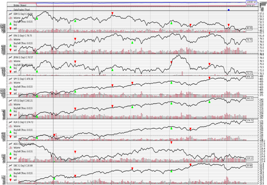
Fig. 6. Result of Universe 1 by Backtrader. The results indicate that the proposed algorithm is more effective at identifying upward trends than downward trends, which may be attributed to the tendency of linear models to preserve momentum during sustained upward movements, while exhibiting delayed responses at abrupt market downturns due to their reliance on historical averages. The performance accounting for transaction costs (\(=0.001\)) is shown in the upper section of the figure, with an initial capital of USD 100,000.
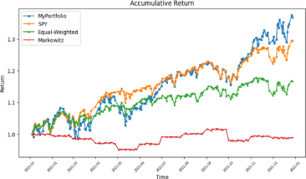
Fig. 7. Result of Universe 1.
For the four investment portfolios, the annualized return, SR, Sortino ratio, and maximum drawdown were calculated in Table 10. While the proposed algorithm achieved the highest return among all strategies, it showed slightly lower stability compared to SPY in terms of volatility and drawdown. Nevertheless, it outperformed the other portfolios across multiple performance indicators, demonstrating a strong overall balance between return and risk.
| Portfolio | Return | Volatility | SR | Sortino ratio | Max drawdown |
| MyPortfolio | 0.4008 | 0.1875 | 2.0841 | 3.1567 | 0.0877 |
| SPY | 0.3205 | 0.1324 | 2.3454 | 3.3289 | 0.0542 |
| Equal-weighted | 0.1820 | 0.1163 | 1.4795 | 2.0350 | 0.0481 |
| Markowitz | \(-0.0125\) | 0.0642 | \(-0.3513\) | \(-0.3688\) | 0.0523 |
To evaluate robustness under different market regimes, we conduct an extended backtest on Universe 1 from 2018 to 2022 (Fig. 8 and Table 11). The proposed model achieves competitive performance, with a SR (0.79) comparable to SPY, while outperforming the equally weighted and Markowitz portfolios in both return and risk-adjusted metrics. Although slightly underperforming SPY in annualized return, it demonstrates a better balance between return and risk than the Markowitz model and improved stability compared to naive allocation. Overall, the results indicate that the proposed method maintains stable and robust performance across diverse market conditions.
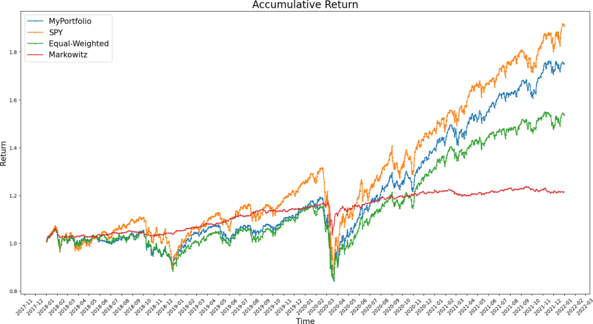
Fig. 8. Result of Universe 1 (2018–2022).
| Portfolio | Return | Volatility | SR | Sortino ratio | Max drawdown |
| MyPortfolio | 0.1502 | 0.1772 | 0.7914 | 0.8489 | 0.2950 |
| SPY | 0.1752 | 0.2080 | 0.7942 | 0.8908 | 0.3372 |
| Equal-weighted | 0.1134 | 0.1623 | 0.6369 | 0.7086 | 0.2725 |
| Markowitz | 0.0498 | 0.0532 | 0.7492 | 0.7217 | 0.1165 |
5.2.2. Result of Universe 2
The blue line represents the backtest performance of the proposed algorithm, the orange line corresponds to SPY, the green line to the equally weighted strategy, and the red line to the MV model (Fig. 9). When the universe is selected randomly, the model’s performance slightly declines; however, it still outperforms both the equally weighted strategy and the MV model.
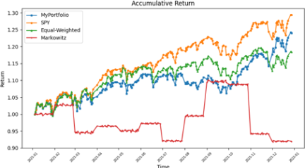
Fig. 9. Result of Universe 2.
For the four investment portfolios, the annualized return, SR, Sortino ratio, and maximum drawdown were calculated in Table 12. The proposed algorithm achieved a return of 26%, but exhibited lower stability compared to SPY and the equally weighted strategy. However, it demonstrated significantly better performance than the MV model.
| Portfolio | Return | Volatility | SR | Sortino ratio | Max drawdown |
| MyPortfolio | 0.2618 | 0.1343 | 1.8755 | 2.8204 | 0.0522 |
| SPY | 0.3205 | 0.1324 | 2.3454 | 3.3289 | 0.0542 |
| Equal-weighted | 0.2001 | 0.1316 | 1.4446 | 1.9880 | 0.0581 |
| Markowitz | \(-0.0876\) | 0.2255 | \(-0.4327\) | \(-0.4170\) | 0.1657 |
5.2.3. Result of Universe 3
The blue line represents the backtest performance of the proposed algorithm, the orange line corresponds to SPY, the green line to the equally weighted strategy, and the red line to the MV model (Fig. 10).
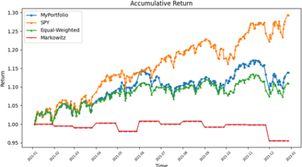
Fig. 10. Result of Universe 3.
As the number of assets increased to 266, the model increasingly tended toward an equally weighted portfolio during training, and gradient explosion was observed. To address these issues, L2 regularization was introduced and a Dropout layer was added after the LSTM layer. In addition, to reduce computational cost given the large volume of data, an early stopping strategy was also employed.
The results from Universe 3 (Table 13) indicate that as the number of assets increases, the model tends to shift toward an equally weighted portfolio, failing to effectively implement stock selection. While this behavior achieves a certain level of diversification, it suggests that the model does not fully leverage the capabilities of artificial intelligence for asset selection, highlighting an area for potential improvement in future research.
| Portfolio | Return | Volatility | SR | Sortino ratio | Max drawdown |
| MyPortfolio | 0.1504 | 0.1228 | 1.1439 | 1.5737 | 0.0670 |
| SPY | 0.3205 | 0.1324 | 2.3454 | 3.3289 | 0.0542 |
| Equal-weighted | 0.1189 | 0.1069 | 1.0187 | 1.4441 | 0.0539 |
| Markowitz | \(-0.0486\) | 0.0636 | \(-0.9212\) | \(-0.8024\) | 0.0529 |
6. Conclusion and Future Work
6.1. Conclusion
This study proposes a two-stage portfolio optimization framework integrating return prediction and allocation learning. Empirical results across multiple asset universes demonstrate that the proposed method consistently outperforms traditional baselines, including equal-weighted and mean-variance portfolios, in terms of risk-adjusted performance.
While the model does not always exceed the SPY benchmark in raw returns and may exhibit lower stability in certain scenarios, it achieves competitive SRs and improved downside resilience, indicating a more balanced trade-off between return and risk. Notably, in large-scale universes, the method maintains robustness across different market regimes, as evidenced by the extended backtest over 2018–2022.
However, two limitations remain. First, the predictive performance of DLinear degrades for highly volatile assets. Second, as the asset universe expands, the allocation model tends to converge toward near-equal weighting, suggesting limited differentiation in high-dimensional settings.
Overall, the proposed framework provides a stable and scalable approach to portfolio optimization, offering consistent improvements over classical methods while highlighting key directions for future refinement.
6.2. Future Work
Future research could explore several promising directions. First, replacing the dataset with one that represents a broader market scope, such as the SPDR S&P 500 ETF, may allow for performance evaluation under more diverse asset environments. Alternatively, using data from policy-sensitive markets, such as China, could help assess the model’s robustness under highly volatile and government-influenced conditions.
In terms of feature selection, this study relied on default indicators provided by the yfinance library. Future work could enhance model inputs by incorporating additional financial factors, including moving averages of ETF prices, PBR, PER, and return on equity. Furthermore, applying sentiment analysis to economic news and using sentiment scores as input features offer a promising way to integrate textual data into the modeling pipeline.
For the prediction model, adopting time-series forecasting techniques specifically designed for financial data may improve accuracy. On the optimization side, the objective function could be extended with penalty terms that better capture the trade-off between return and risk, offering more flexible and realistic portfolio allocation.
With regard to investment strategy design, additional constraints could be introduced, such as filtering out assets with low expected returns. Moreover, a preliminary stock selection step using machine learning techniques could help identify low-risk assets for constructing a more robust investment universe.
Finally, the current model required over one hour to process a universe of 266 assets. As the dataset scales, computational cost may become a bottleneck. Thus, future work could consider algorithmic simplification or the use of distributed computing to improve scalability and efficiency in large-scale applications.
- [1] H. Markowitz, “Portfolio selection,” The J. of Finance, Vol.7, No.1, pp. 77-91, 1952. https://doi.org/10.2307/2975974
- [2] W. F. Sharpe, “Mutual fund performance,” The J. of Business, Vol.39, No.S1, pp. 119-138, 1966. https://doi.org/10.1086/294846
- [3] W. F. Sharpe, “Capital asset prices: A theory of market equilibrium under conditions of risk,” The J. of Finance, Vol.19, No.3, pp. 425-442, 1964. https://doi.org/10.2307/2977928
- [4] F. Black and R. B. Litterman, “Asset allocation: Combining investor views with market equilibrium,” The J. of Fixed Income, Tech. Rep.2, 1991. https://doi.org/10.3905/jfi.1991.408013
- [5] I. Karatzas and R. Fernholz, “Stochastic portfolio theory: An overview,” A. Bensoussan and Q. Zhang (Eds.), “Handbook of Numerical Analysis,” Vol.15, pp. 89-167, 2009. https://doi.org/10.1016/S1570-8659(08)00003-3
- [6] X. Hou, K. Wang, J. Zhang, and Z. Wei, “An enriched time-series forecasting framework for long-short portfolio strategy,” IEEE Access, Vol.8, pp. 31992-32002, 2020. https://doi.org/10.1109/access.2020.2973037
- [7] I. S. Chaudhry, F. Farooq, and A. Mushtaq, “Factors affecting portfolio investment in Pakistan: Evidence from time series analysis,” Pakistan Economic and Social Review, pp. 141-158, 2014.
- [8] H. K. Choi, “Stock price correlation coefficient prediction with arima-lstm hybrid model,” arXiv:1808.01560, 2018. https://doi.org/10.48550/arXiv.1808.01560
- [9] W. Wang, W. Li, N. Zhang, and K. Liu, “Portfolio formation with preselection using deep learning from long-term financial data,” Expert Systems with Applications, Vol. 143, Article No.113042, 2020. https://doi.org/10.1016/j.eswa.2019.113042
- [10] Z. Zhang, S. Zohren, and S. Roberts, “Deep learning for portfolio optimization,” The J. of Financial Data Science, Vol.2, No.4, pp. 8-20, 2020. https://doi.org/10.3905/jfds.2020.1.042
- [11] A. Filos, “Reinforcement learning for portfolio management,” arXiv:1909.09571, 2019. https://doi.org/10.48550/arXiv.1909.09571
- [12] Z. Jiang, D. Xu, and J. Liang, “A deep reinforcement learning framework for the financial portfolio management problem,” arXiv:1706.10059, 2017.
- [13] S. Pyo and J. Lee, “Exploiting the low-risk anomaly using machine learning to enhance the Black–Litterman framework: Evidence from South Korea,” Pacific-Basin Finance J., Vol.51, pp. 1-12, 2018. https://doi.org/10.1016/j.pacfin.2018.06.002
- [14] J. Shi, M. Jain, and G. Narasimhan, “Time series forecasting (TSF) using various deep learning models,” arXiv:2204.11115, 2022. https://doi.org/10.48550/arXiv.2204.11115
- [15] A. N. Elmachtoub and P. Grigas, “Smart predict, then optimize: Decision-focused learning using label-aware losses,” Management Science, Vol.67, No.9, pp. 5752-5771, 2021.
- [16] J. Mandi, J. Kotary, S. Berden, M. Mulamba, V. Bucarey, T. Guns, and F. Fioretto, “Decision-focused learning: Foundations, state of the art, benchmark and future opportunities,” J. of Artificial Intelligence Research, Vol.80, pp. 1623-1701, 2024. https://doi.org/10.1613/jair.1.15320
- [17] A. Vaswani et al., “Attention is all you need,” Advances in Neural Information Processing Systems, Vol.30, 2017.
- [18] H. Zhou, S. Zhang, J. Peng, S. Zhang, J. Li, H. Xiong, and W. Zhang, “Informer: Beyond efficient transformer for long sequence time-series forecasting,” Proc. of the AAAI Conf. on Artificial Intelligence, Vol.35, No.12, pp. 11106-11115, 2021. https://doi.org/10.1609/aaai.v35i12.17325
- [19] H. Wu et al., “Autoformer: Decomposition transformers with auto-correlation for long-term series forecasting,” Advances in Neural Information Processing Systems, Vol.34, pp. 22419-22430, 2021.
- [20] A. Zeng, M. Chen, L. Zhang, and Q. Xu, “Are transformers effective for time series forecasting?,” Proc. of the AAAI Conf. on Artificial Intelligence, Vol.37, No.9, pp. 11121-11128, 2023. https://doi.org/10.1609/aaai.v37i9.26317
- [21] S. Hochreiter and J. Schmidhuber, “Long short-term memory,” Neural Computation, Vol.9, No.8, pp. 1735-1780, 1997. https://doi.org/10.1162/neco.1997.9.8.1735
This article is published under a Creative Commons Attribution-NoDerivatives 4.0 Internationa License.