
Research Paper:
An Interactive Remaining Useful Life Estimation Method for Lithium-Ion Batteries Based on Composite Performance Index and Nonlinear Wiener Process
Shisheng Fu*1, Ruifeng Chen*2, Xiao He*3, Hangfeng Guo*4, Baokang Zhang*1
 , Qi Wu*1,†
, and Wen-An Zhang*1
, Qi Wu*1,†
, and Wen-An Zhang*1
*1Zhejiang University of Technology
No.288 Liuhe Road, Hangzhou, Zhejiang 310023, China
†Corresponding author
*2Zhejiang Zhongchai Machine Co., Ltd.
No.1 Meixi Road, Shaoxing, Zhejiang 312532, China
*3University of Pennsylvania
3451 Walnut Street Philadelphia, PA 19104, USA
*4Zhejiang Hengjiu Transmission Technology Inc., Ltd.
No.27 Qianxi Road, Taozhu Street, Zhuji, Zhejiang 311800, China

A framework integrating deep learning and nonlinear Wiener process (NWP) is proposed for the remaining useful life prediction of lithium-ion batteries. First, degradation features from multi-source sensor data are automatically extracted using an autoencoder incorporating embedded L1 regularization. Second, a one-dimensional composite performance indicator is constructed via neural networks to accurately describe the performance degradation trajectory of the battery. Subsequently, a stochastic degradation model based on the NWP is established, wherein complex degradation dynamics are effectively captured by a time-varying drift function. On this basis, a Bayesian posterior update mechanism is integrated to adaptively adjust model parameters online, whereby individual differences are quantified. Finally, experimental verification on public datasets demonstrates that the proposed method reduces root mean square error and mean absolute error by more than 20%, and significant improvements in prediction accuracy are achieved via the data-model interaction architecture that combines feature compression, degradation quantification, and parameter adaptation.
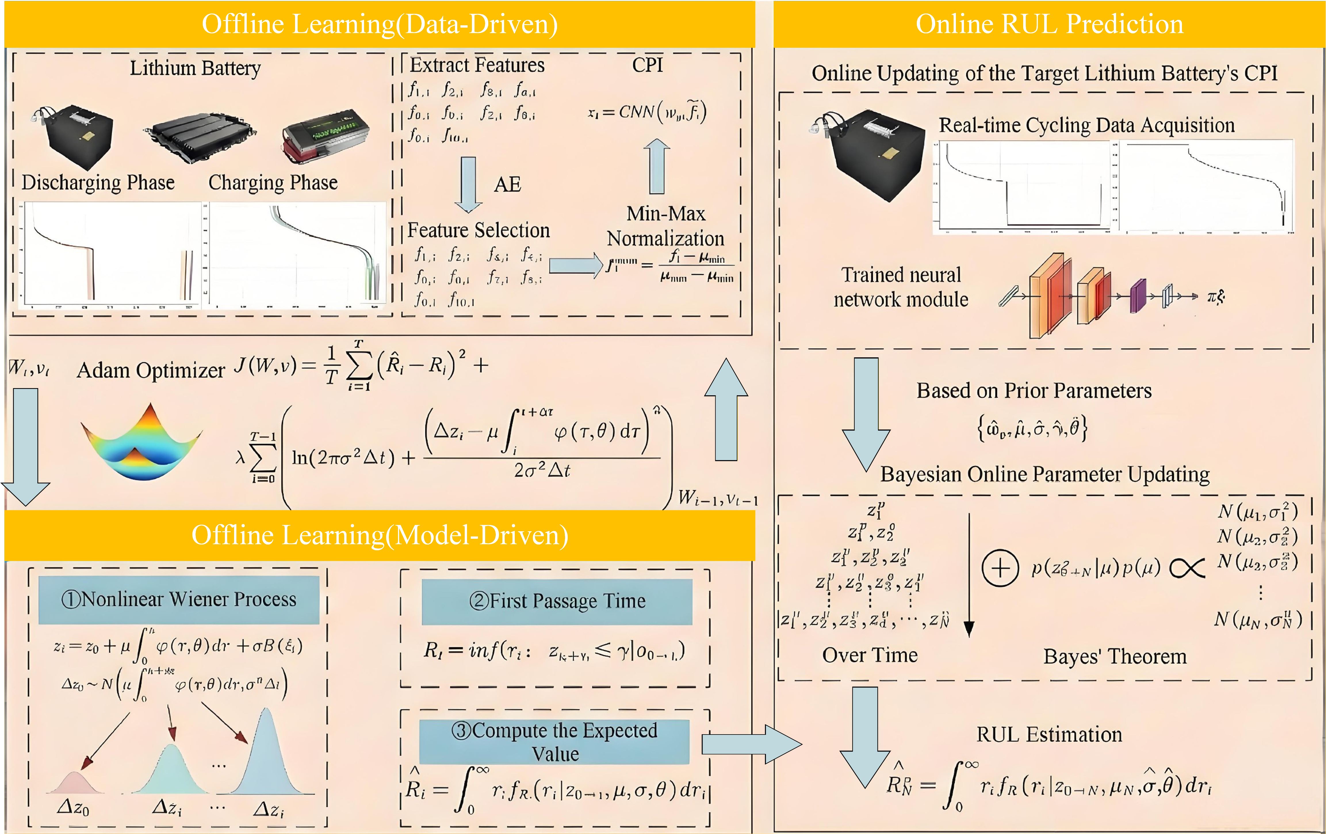
Framework of the proposed RUL method
1. Introduction
Lithium-ion batteries, recognized for being highly energy-efficient, long-life, and lightweight, are widely utilized in electric vehicles, military equipment, and other fields 1. However, due to the non-linear characteristics of the electrochemical system, battery performance is rendered sensitive to factors such as operating temperature, charge or discharge current, and depth of discharge. Consequently, gradual performance degradation may be induced, by which serious safety hazards, such as internal short circuits and thermal drift, are caused, and the stable operation of the equipment is threatened 2. Furthermore, lithium-ion batteries are subjected to prolonged high-load conditions via frequent charge-discharge cycles, wherein electrode material aging and electrolyte decomposition are accelerated, and the remaining useful life (RUL) is further reduced 3. RUL estimation is considered one of the key technologies in prognostics and health management, by which an estimate of RUL can be obtained before failure occurs 4. Therefore, extensive attention has been paid to the study of RUL estimation for lithium-ion batteries by both academic and industrial fields.
Existing methods for predicting the RUL of lithium-ion batteries can be broadly categorized into two main groups: physical model-driven and data-driven approaches 5. In the former, the dynamic degradation behavior of lithium-ion batteries is described by establishing electrochemical or equivalent circuit models, and the state of charge (SOC) is estimated through parameter identification. For instance, an improved Thevenin mixed equivalent circuit model was proposed by Chen et al. 6, by which accurate state estimation of lithium-ion batteries is achieved. Similarly, a fractional-order impedance model was constructed by Sun and Wang 7 through the analysis of impedance spectroscopy to improve SOC estimation. Nevertheless, these methods are primarily focused on real-time state estimation, and multi-step information is not effectively integrated for the prediction of long-term degradation trends. To address this, a multi-model Gaussian process method was proposed by Li et al. 8, in which multiple candidate capacity degradation models are incorporated to capture the multi-stage capacity degradation trend of the batteries. However, heavy reliance is placed on complex model parameters within lithium batteries by such methods; the precise determination of microscopic data, such as electrolyte diffusion coefficients and the kinetic parameters of the electrode reaction, is required, alongside the creation of highly complex mathematical models to simulate internal electrochemical reactions and mass transfer processes.
With the rapid advancement of big data and intelligent sensor technologies, the acquisition of monitoring data related to the degradation process of lithium-ion batteries has become increasingly facilitated, providing a robust data foundation for data-driven RUL estimation. By directly learning degradation patterns from historical data, these methods establish complex mapping relationships between input parameters and the RUL. Currently, various network architectures, such as convolutional neural networks (CNN), long short-term memory (LSTM) 9, and deep belief networks (DBN) 10, have been widely implemented. To further enhance model generalization and interpretability, recent research focus has shifted toward the deep integration of physical mechanisms with data-driven approaches. For instance, researchers have utilized physics-informed neural networks (PINN) to collaboratively constrain the prediction of degradation trajectories, thereby balancing the rigor of physical laws with the powerful fitting capabilities of neural networks 11,12. Meanwhile, addressing the multi-scale characteristics of battery degradation, multimodal deep learning frameworks that fuse time-frequency domain health features have proven effective in improving prediction accuracy 13. Furthermore, considering the computational constraints of embedded battery management systems (BMS), lightweight architectures such as the lightweight deformable network (LDNet) have significantly reduced model complexity while maintaining high precision 14. However, the aforementioned methods primarily quantify epistemic uncertainty arising from limited data and noise, rather than the aleatory uncertainty induced by the inherent stochasticity of the degradation process. Consequently, such quantification results still fail to truly reflect the underlying stochastic degradation dynamics.
Inspired by the respective advantages of stochastic process model-driven and data-driven methods, significant research efforts have been dedicated to developing RUL prediction approaches that integrate these two paradigms. For instance, a method for RUL estimation was proposed by Dai et al. 15, in which health indicators characterizing the degradation trend are extracted from multi-source sensor monitoring data, and a linear Wiener process is employed to model the performance degradation of lithium-ion batteries. Similarly, DBN and hidden Markov models were integrated by Peng et al. 16 utilizing multisource equipment monitoring data; specifically, the former is utilized to establish a mapping between monitoring data and health indicators, while the latter is employed to simulate degradation dynamics. However, in these methods, degradation feature extraction and stochastic modeling are often performed independently, leading to a feature-model mismatch that diminishes the accuracy of RUL estimation. To address this, a solution for predicting the RUL of stochastic degradation devices based on a data-model interactive framework was proposed by Wu et al. 17. In this framework, a cost function is constructed based on the discrepancy between actual and predicted life to establish a link between composite health indicators and RUL, thereby enhancing estimation accuracy. Nevertheless, complex nonlinear characteristics are frequently exhibited by the actual degradation process; consequently, these dynamic changes may not be accurately captured by standard linear Wiener models, and the accuracy of RUL predictions is thereby compromised.
The aforementioned challenges have motivated the present study, in which a method for RUL estimation of lithium-ion batteries is proposed. First, multi-source sensor data covering the entire lifecycle are collected, and multi-dimensional degradation features are extracted via the integration of time-frequency domain statistics. Subsequently, these degradation features are processed using an autoencoder (AE) network, through which sensitive feature subsets characterizing the battery degradation state are automatically extracted. On this basis, a composite performance index (CPI) is constructed via a neural network to characterize the trend of battery performance degradation. Next, a stochastic degradation model accounting for unit-to-unit variability is established based on the nonlinear Wiener process (NWP), and the corresponding point estimation and variance parameters are derived to capture the dynamics of the CPI. Thereafter, a joint objective function integrating the mean squared error of the RUL estimation and the log-likelihood of the stochastic process is formulated, by which the synchronous optimization of the CPI and stochastic degradation modeling is achieved. Finally, the parameters of the nonlinear Wiener process are updated via a Bayesian online update mechanism to quantify the uncertainty associated with the target battery and to realize the online prediction of its RUL. To verify the effectiveness and superiority of the proposed method, experiments are conducted using the University of Maryland lithium-ion battery datasets.
The main contributions of this paper are summarized as follows:
-
1.
In contrast to 17, a time-varying drift term based on a double exponential kernel function was introduced in the degradation model, which can effectively model the non-stationary degradation characteristics of lithium-ion batteries during their degradation process.
-
2.
The core parameters of the stochastic degradation model are embedded into the loss function of neural network, with the degradation model parameters optimized synchronously via gradient descent. This method mitigates parameter-model fitting errors and eliminates the need for complex iterative calculations.
-
3.
A data-model interaction framework is developed for predicting the RUL of lithium-ion batteries. By means of feature compression, degradation quantification, and Bayesian parameter updating modules, it realizes the fusion of multi-sensor data and stochastic degradation models, thereby quantifying individual differences like the aging of lithium-ion batteries.
2. Preliminaries
2.1. AE
An AE is characterized as a neural network architecture designed to extract low-dimensional features from data through unsupervised learning 15. Its fundamental objective is established as the minimization of the error between the input data and the reconstructed output. Structurally, the model is composed of two distinct components: an encoder and a decoder. Within this framework, input data are compressed by the encoder into low-dimensional features residing in a latent space, while the original input is reconstructed by the decoder based on this encoded representation, with the aim of maximizing fidelity to the source data.
Given the input space \(X\in \mathcal{X}\) and feature space \(h\in \mathcal{F}\), the AE solves the mapping \(f\), \(g\) between the two to minimize the reconstruction error of the input features.
The output of the encoder, namely the hidden layer feature \(h\), can be regarded as the representation of the input data.
2.2. Wiener Process
The Wiener process, also referred to as Brownian motion, is recognized as a representative stochastic process model characterized by continuous-time parameters and a continuous state space. By virtue of its distinctive properties—namely, independent increments, the Markov property, and its applicability to non-monotonic degradation behaviors—it has been extensively applied within the fields of lithium-ion battery degradation modeling and RUL estimation 16.
If a stochastic process \(\{ \hat{z}_t, t \geq 0 \}\) satisfies the following conditions, it is called a Wiener process:
-
1.
\(\hat{z}_t\) is an incremental process;
-
2.
\(\forall s,t>0\), increment \(\hat{z}_{s+t}-\hat{z}_t\sim N(0,c^2t)\), i.e., the increment follows a normal distribution with a mean of 0 and a variance of \(c^2t\).
-
3.
\(\hat{z}_t\) is a continuous function of \(t\).
In this paper, the time-varying degradation process of lithium-ion batteries is modeled using a nonlinear Wiener process driven by standard Brownian motion 17,18,19. The dynamic characteristics of complex degradation systems are more accurately characterized by this approach. The nonlinear Wiener process is defined as an extended form of the standard Wiener process. Through the introduction of a nonlinear drift function and a stochastic diffusion term, the dynamic behavior of complex degradation systems is described with greater precision, and the model is given by:
3. Methodology
The framework of the proposed method is illustrated in Fig. 1. The method initiates with data preparation: sensor data spanning the full lifecycle of batteries is collected, followed by multidimensional feature extraction using time-frequency domain statistics and preprocessing (e.g., min-max normalization). Subsequently, an AE processes the features to distill a sensitive subset characterizing degradation states. The refined features are then fed into a neural network to construct a one-dimensional CPI. Based on the CPI, a stochastic degradation model incorporating individual differences is established via the nonlinear Wiener process, with corresponding point estimates derived. Crucially, a joint optimization function—integrating the mean squared error of RUL estimation and the log-likelihood of the stochastic process—enables simultaneous optimization of the CPI and degradation model parameters. Finally, the nonlinear Wiener process parameters are dynamically updated using a Bayesian online mechanism 20, allowing online RUL prediction for target lithium-ion batteries under real operational conditions.
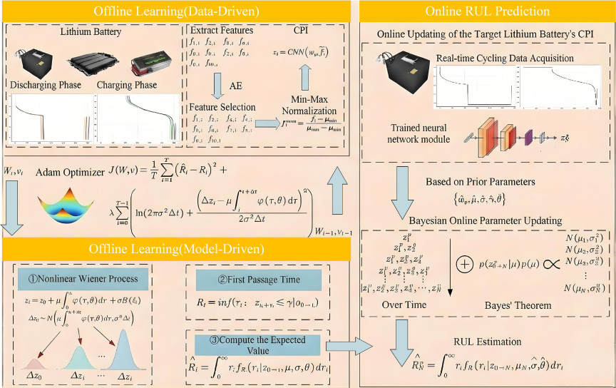
Fig. 1. Framework for predicting RUL of lithium-ion batteries.
3.1. Preprocessing of Data
For lithium-ion battery monitoring equipment equipped with multiple sensors, during a complete charge-discharge cycle, it is assumed that there are \(K\) sensors that perform measurements at time instants \(t=\{t_1,t_2,t_3,\ldots,t_J \}\), resulting in a total of \(J\) sampling moments. It is assumed that all sensors have identical sampling frequencies, and the time interval between two consecutive sampling instants is constant and equal to \(\Delta t=t_{j+1}-t_j\), where \(j\) denotes the index of the \(j\)-th sampling moment. Let \(X_i\) denote the historical dataset of the \(i\)-th charge-discharge cycle, whose elements are \(X^{t}_{i,k}\), where \(i\) represents the \(i\)-th cycle, \(k\) represents the \(k\)-th sensor (\(1\leq k\leq K\)), and \(j\) represents the \(j\)-th sampling point (\(1\leq j\leq J\)). Thus, \(X_i\) can be expressed as:
3.2. Unsupervised Feature Selection Based on AE
The redundancy and nonlinear coupling characteristics of high-dimensional sensor data severely constrain model performance, while traditional feature selection methods rely on manual design and are unable to effectively capture complex degradation patterns. Based on the unsupervised feature selection mechanism of AEs, the importance of features is automatically quantified under unlabeled conditions through learnable weights and L1 regularization mechanisms. The encoder–decoder structure is used to implicitly extract nonlinear low-dimensional representations, thereby achieving feature sparsity and data reconstruction. This method not only avoids the limitations of label dependency and linear assumptions, but also preserves the essential structure of the data, providing an efficient and interpretable feature selection solution for industrial scenarios, significantly improving the robustness and computational efficiency of degraded modeling. Specifically, apply the learnable weight vector \(w\in \mathbb{R} ^N\) to the normalized training set feature vector \(\boldsymbol{f}^{\mathrm{norm}}\) to generate a weighted feature representation:
The AE reconstructs features from latent representations: it maps features to a latent space \(\boldsymbol{z}\in \mathbb{R} ^d\) (\(d\ll N\)), then reconstructs them to the original feature space. The training objective is jointly optimized by reconstruction error and regularization term:
3.3. Nonlinear Wiener Process Modeling Based on CNN
Input the selected feature vector \(\tilde{\boldsymbol{f}}\) into the CNN network to obtain CPI:
The maximum likelihood estimation for the nonlinear Wiener process is given by:
The technical essence of this formulation lies in the synchronous optimization of the feature mapping and the degradation modeling parameters. Unlike traditional sequential methods where feature extraction and stochastic modeling are decoupled, this joint objective function treats the neural network’s output, CPI, not merely as a regression target but as a stochastic process variable that must strictly adhere to the statistical properties of an NWP.
Specifically, the first term (MSE) ensures the global trend of the extracted CPI matches the actual RUL trajectory. Simultaneously, the second term, \(\mathcal{L}_{\text{WP}}\), regularizes the local increments of the CPI to follow the Gaussian distribution defined by the NWP. By minimizing \(J\) via gradient descent, the CNN learns to filter out non-degradation-related noise while the NWP parameters adaptively capture the underlying stochastic dynamics.
Through this simultaneous optimization process, the model yields the optimal parameter set \(\{ \hat{w}_g,\hat{\mu},\hat{\sigma},\hat{\gamma},\hat{\theta}\}\), where \(\hat{w}_g\) denotes the optimal weights in the convolutional neural network, \(\hat{\mu}\) represents the optimal mean drift coefficient in the nonlinear Wiener process, \(\hat{\sigma}\) is the optimal diffusion coefficient, \(\hat{\gamma}\) denotes the optimal failure threshold, \(\hat{\theta}\) indicates the optimal function parameters.
Simultaneously, a series of CPI \(z_{0\rightarrow T}\) is obtained. The unit-to-unit variability of lithium-ion batteries is characterized by the standard deviation of the drift coefficient, w.l.o.g., it satisfies the normal distribution \(\mu \sim N(\hat{\mu },\sigma _{\mu}^{2})\), where
3.4. Online RUL Estimation Based on Bayesian Posterior Updating
After obtaining the prior parameters, individualized prediction is further realized through Bayesian updating. The feature vector, extracted from the target lithium-ion battery and normalized, is input into the convolutional neural network to obtain a series of \(z_{0\rightarrow N}^{p}\) representing the CPI from the initial time to the current time and \(\mu \sim N(\hat{\mu },\sigma _{\mu}^{2})\) as the prior. The Bayesian posterior update is used to update the drift coefficient to quantify the individual variability value of different lithium-ion batteries:
The Bayesian posterior updating process establishes a dynamic bidirectional feedback loop between the empirical data and the degradation model. During the online phase, the offline-trained stochastic degradation model provides the prior degradation rules. As sequential monitoring data from the target battery are continuously acquired, the neural network extracts real-time composite performance indicators to serve as data evidence. Through Bayesian inference, this real-time data dynamically correct the drift coefficient of the model, quantifying the specific aging characteristics of individual batteries. Conversely, the updated stochastic model imposes theoretical constraints on the real-time data, filtering out local measurement noise and guiding the subsequent RUL extrapolation. This continuous fusion of real-time data streams and stochastic processes constitutes the core interaction mechanism of the proposed framework.
3.5. Algorithm Implementation
The proposed framework for estimating the remaining life of lithium-ion batteries consists of three core modules: unsupervised feature selection based on AEs, nonlinear Wiener process random degradation modeling, and a Bayesian parameter adaptation mechanism. The overall process can be summarized as Algorithm 1.
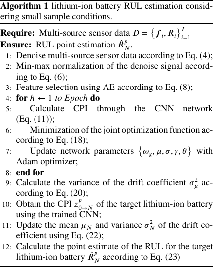
First, multi-source intelligent sensor data from lithium-ion batteries are collected. After extracting time-domain and frequency-domain features from the original data, normalization operations are performed. Subsequently, a one-dimensional CPI characterizing the degradation state of lithium-ion batteries is obtained using a CNN. Then, a stochastic degradation model is established to model the CPI at any initial degradation level, quantifying the uncertainties of the degradation state over time and individual differences. An optimization function with nonlinear Wiener process constraints is constructed, and parameters are continuously updated. After obtaining the optimal parameters, the mean and variance of the drift coefficient are updated using Bayesian theory. Finally, the RUL value of the target lithium-ion battery is estimated online through the updated mean and variance.
4. Experiment
To demonstrate the effectiveness and superiority of the proposed method, the University of Maryland lithium-ion battery dataset 7 was used as the case study test dataset. The case study was conducted the PyTorch 1.13.0 framework on a computer equipped with an Intel Core i7-12700H, NVIDIA RTX 3060, and 32 GB RAM.
4.1. Data Description
4.1.1. Battery Aging Datasets
The experimental validation of the proposed framework is conducted using the lithium-ion battery aging dataset provided by the Center for Advanced Life Cycle Engineering (CALCE) at the University of Maryland 25. The study focuses on 18650-type lithium-ion cobalt oxide batteries—specifically samples CS2\(\_\)35, CS2\(\_\)36, CS2\(\_\)37, and CS2\(\_\)38—which underwent cyclic charge-discharge aging tests at a \(C/2\) rate within a temperature-controlled environment. Throughout the aging process, time-series data for voltage, current, and battery temperature were continuously monitored at sampling rates ranging from 1 Hz to 1 kHz. The state of health is defined by capacity fading, with the end-of-life (EOL) threshold reached when the discharge capacity drops to 70\(\%\) of its nominal value. Each battery in the study completed approximately 700 cycles, enabling comprehensive full-lifecycle performance monitoring.
To further validate the universality and robustness of the proposed framework, additional experiments are conducted using Batch-1 of the public lithium-ion battery dataset provided by Xi’an Jiaotong University (XJTU) 26. The experimental protocol for this dataset consists of an initial calibration cycle followed by continuous accelerated degradation cycles. During the initial calibration, the battery is charged in constant current (CC) mode at 1 A until the voltage reaches a cut-off of 4.2 V. It then switches to constant voltage (CV) mode at 4.2 V until the current attenuates to 0.04 A, followed by a 5-minute rest. Subsequently, the battery is discharged in CC mode at 0.4 A down to 2.5 V, concluding with another 5-minute rest. For the accelerated degradation phase, a more aggressive profile is applied; the battery is charged in CC mode at 4 A to 4.2 V, switched to CV mode at 4.2 V until the current drops to 0.1 A, and rested for 5 minutes. The discharge phase is then executed in CC mode at 2 A until the voltage degrades to 2.5 V, followed by a final 5-minute rest. These accelerated cycles are repeated continuously until the battery reaches the end of its aging process.
4.1.2. Design of Nonlinear Drift Function
A double-exponential kernel function, \(e^{\alpha t} + e^{\beta t}\), is integrated into the NWP model to capture the complex nonlinear degradation characteristics inherent in these datasets 24,27. In this formulation, the first exponential term simulates long-term progressive decay, primarily driven by the loss of lithium inventory and electrode active material, while the second term captures non-stationary fluctuations and accelerated aging phenomena observed at specific life stages. This hybrid mathematical approach provides the necessary flexibility to accurately fit diverse aging trajectories over the lifespans. By grounding the stochastic process in these electrochemical insights, the model maintains high consistency with real-world degradation laws, thereby significantly improving the reliability of RUL predictions.
4.2. Data Preparation and Preprocessing
Step 1: From the full-life cycle experiments, CS2\(\_\)35, CS2\(\_\)36, CS2\(\_\)37, and CS2\(\_\)38 were selected as experimental samples. The charge-discharge cycles were conducted as follows, in the charging phase, a CC (1 A) was applied until the cut-off voltage of 4.2 V was reached, followed by a CV (4.2 V) charging until the current decayed to 0.04 A, and then a 5-minute rest period. In the discharging phase, a CC (0.4 A) was applied until the voltage decayed to 2.5 V, followed by another 5-minute rest period; this entire process constituted one cycle. The four batteries all had a rated capacity of 2 mAh, so the EOL was set at a capacity decay to 1.4 mAh. Additionally, pairwise tests were performed on the batteries and CS2\(\_\)35 was used as historical data while CS2\(\_\)36 as test data, and then CS2\(\_\)36 was used as historical data while CS2\(\_\)35 as test data. Similarly, the same operations were carried out for CS2\(\_\)37 and CS2\(\_\)38.
Step 2: Based on the degradation data, 10 features in both time and frequency domains were extracted for predicting the RUL of lithium-ion batteries. These features include charge/discharge internal resistance, CC charging time, CV charging time, total spectral energy during CV charging, total spectral energy during CC discharging, average current slope during CV charging, average voltage slope during CC discharging, current decay time, voltage decay time, mean current during CV charging, and mean voltage during CC discharging.
Specifically, time-domain and frequency-domain features were extracted from the raw data. Subsequently, based on the AE module, degradation features most relevant to the degradation trend were selected. This aims to retain key information about the degradation trend, while reducing interference from redundant data and improving processing efficiency. On the other hand, using the screened features, a CNN network was employed to fuse multi-source information and construct a one-dimensional CPI that describes the degradation trend of lithium-ion batteries.
4.3. Comparison Methods and Parameter Configuration
The following methods are selected as the baseline methods for the University of Maryland lithium-ion battery dataset.
-
1)
LSTM 28: LSTM adopts a three-layer architecture. The first layer is an LSTM hidden layer with 64 nodes; the second layer is an LSTM hidden layer with 32 nodes; the third layer is a fully connected output layer with 1 node, which is used for RUL prediction.
-
2)
GRU 29: The network adopts a three-layer architecture. The first layer is a GRU hidden layer with 48 nodes; the second layer is a GRU hidden layer with 24 nodes; the third layer is a fully connected output layer with 1 node, which is used for RUL prediction.
-
3)
CNN-NWP-Bayes: The CNN consists of five layers. The first layer is a convolutional layer with 16 output channels and a convolution kernel size of \(3\times3\); the second layer is a convolutional layer with 32 output channels and a convolution kernel size of \(3\times3\); the third layer is a fully connected layer with 16 nodes, using ReLU as the activation function; the fourth layer is a fully connected layer with 8 nodes, using ReLU as the activation function; the fifth layer is a fully connected output layer with 1 node, whose output is used to construct the composite performance indicator for the nonlinear Wiener process degradation model, and prediction is performed in combination with Bayesian updating.
-
4)
AE-CNN-LWP-Bayes: Compared with the proposed method, this method replaces the nonlinear Wiener process module with a linear Wiener process module.
-
5)
AE-MLP-NWP-Bayes: Compared with the proposed method, this method replaces the CNN module with a multi-layer perceptron (MLP) module.
-
6)
AE-CNN-NWP: This method omits the Bayesian update module from the proposed method.
-
7)
Proposed method: In this experiment, a double-exponential function \(e^{\alpha\tau} + e^{\beta\tau}\) is adopted as the kernel function 23,25,26, and a double-exponential type Wiener process model \(z_i = z_0 + {\mu}/{\alpha}(e^{\alpha t_i} - 1) + {\mu}/{\beta}(e^{\beta t_i} - 1) + \sigma B(t_i)\) is obtained. To unify the symbols, \({\mu}/{\alpha}, \alpha, {\mu}/{\beta}, \beta\) are simply denoted as \(\theta_1, \theta_2, \theta_3, \theta_4\). The CNN is composed of two convolutional layers and one fully-connected layer. The number of output channels of the first convolutional layer is 16, and the number of output channels of the second convolutional layer is 32. The size of the convolution kernel is uniformly set to \(3\times3\). The third layer is a fully-connected layer containing 16 nodes, and the ReLU activation function is adopted. The learning rate of the Adam optimizer is set to 0.0005, and the weight decay coefficient is 1e-5. The number of training epochs and the batch size are set to 400 and 32, respectively. In addition, since the parameters \(\{\hat{w}_g, \hat{\mu}, \hat{\alpha}, \hat{\gamma}, \hat{\theta}\}\) are continuously updated during the training process, only the parameter values after model training are provided. Specifically: \(\theta_1 \sim N(0.119953, 0.01619086^2)\), \(\theta_2=-0.000886\), \(\theta_3 \sim N(0.115118, 0.01618360^2)\), \(\theta_4 = -0.000886\), the failure threshold \(\gamma = -0.1457\), and \(\sigma = 0.004340\).
4.4. Evaluation Metrics
To evaluate and compare the performance of the aforementioned RUL estimation methods, the absolute error, mean squared error, and coefficient of determination are used as evaluation metrics.
1) Mean absolute error (MAE):
2) Root mean square error (RMSE)
3) Coefficient of determination (\(R^2\))
4.5. Results Analysis
To verify the effectiveness of the proposed method in estimating the RUL of lithium-ion batteries and quantifying uncertainties, CS2\(\_\)36 was selected for testing. Figs. 2–5 present the RUL estimation results obtained by this method. Fig. 2 illustrates the relationship between the CPI and the failure threshold using the proposed method. Over time, the CPI generally shows a downward trend with small-scale local fluctuations. Specifically, when the CPI falls below the failure threshold for the first time, the failure of the lithium-ion battery can be defined based on this first passage time.
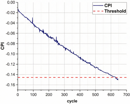
Fig. 2. CPI and threshold.
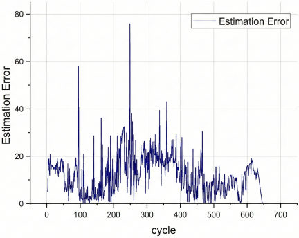
Fig. 3. RUL estimation error (cycles).
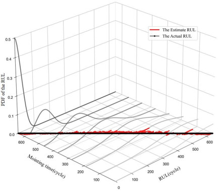
Fig. 4. The predicted RUL and associated PDF.
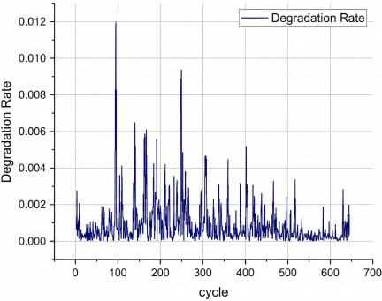
Fig. 5. The rate variation of CPI (cycles).
Figure 3 presents the curve of error variation in the RUL prediction of lithium-ion batteries. It can be observed that the high initial error stems from the insignificant early degradation characteristics and insufficient model learning. The subsequent decrease in error is attributed to the Bayesian update mechanism, which dynamically corrects parameters and fuses the target battery data to quantify individual differences in real time. The convergence of error in the final stage verifies that the nonlinear Wiener process can accurately capture complex degradation dynamics, overcoming the limitation of traditional linear models with fixed degradation rates.
Figure 4 illustrates the characteristics of the probability density distribution for the RUL prediction of lithium-ion batteries under different initial degradation states. It can be seen from the results that there is a high degree of consistency between the predicted values and the true values. As the duration of equipment operation monitoring accumulates, the probability density curve gradually takes on a sharp-peak shape, which reflects that the confidence level of the prediction results continues to improve over time. The experimental results fully verify the reliability and advantages of the method proposed in this paper in handling the problem of stochastic RUL prediction.
Figure 5 demonstrates the characteristics of degradation rate changes in the battery health indicator. Different from the linear Wiener process, which assumes a fixed degradation rate, the nonlinear Wiener process can effectively characterize the mutations, fluctuations, and periodic acceleration or deceleration phenomena existing in the actual degradation process by introducing nonlinear kernel functions. Traditional linear models fail to capture such dynamic changes, which may lead to deviations in life prediction. This state-dependent nonlinear model is more consistent with the real degradation law, thereby improving the prediction accuracy.
The proposed method is compared with baseline methods. Table 1 presents the results of the comparative experiments. It can be observed that the proposed method significantly outperforms existing RUL estimation methods in terms of RMSE. Among them, traditional machine learning methods such as LSTM networks and GRU perform poorly due to their reliance on large amounts of samples. Taking CS2\(\_\)36 as an example, its MAE and RMSE are further reduced by \(9.69\%\) and \(8.23\%\) compared with the optimal comparative method, and the \(R^2\) reaches 0.9939. The AE feature screening module effectively compresses redundancy, reducing the MAE of MLP-NWP-Bayes by \(22.3\%\). The dual exponential kernel nonlinear Wiener process accurately captures the abrupt changes in degradation rate (as shown in Fig. 3), overcoming the limitations of linear models. The Bayesian online update mechanism quantifies the uncertainty of the target lithium-ion battery, enabling online prediction of the remaining life based on the target battery’s data. Finally, this framework achieves an average MAE of 16.00 and an \(R^2\) of 0.9890 on four batteries, fully verifying its effectiveness in achieving RUL prediction in small-sample scenarios.
| Methods | CS2_35 | CS2_36 | CS2_37 | CS2_38 | ||||||||
| MAE | RMSE | \(R^2\) | MAE | RMSE | \(R^2\) | MAE | RMSE | \(R^2\) | MAE | RMSE | \(R^2\) | |
| LSTM | 40.1056 | 39.9792 | 0.9214 | 44.0967 | 54.3986 | 0.9215 | 28.2894 | 35.4587 | 0.9697 | 31.9127 | 40.9604 | 0.9617 |
| GRU | 41.9171 | 44.2104 | 0.9136 | 24.4000 | 30.5762 | 0.9720 | 21.2806 | 25.0955 | 0.9848 | 18.4689 | 22.2868 | 0.9887 |
| CNN-NWP-Bayes | 35.2509 | 44.0902 | 0.9429 | 17.9601 | 25.3580 | 0.9813 | 15.6563 | 22.5733 | 0.9880 | 19.6967 | 25.7590 | 0.9852 |
| AE-CNN-LWP-Bayes | 27.3651 | 31.3721 | 0.9663 | 16.9121 | 18.3126 | 0.9917 | 17.2354 | 20.1568 | 0.9903 | 19.5156 | 23.4156 | 0.9899 |
| AE-MLP-NWP-Bayes | 24.2656 | 29.9172 | 0.9737 | 13.2134 | 15.7952 | 0.9925 | 14.3066 | 16.7213 | 0.9934 | 14.3080 | 20.5793 | 0.9906 |
| AE-CNN-NWP | 23.7725 | 28.6127 | 0.9741 | 17.8082 | 22.2054 | 0.9857 | 16.2135 | 18.4648 | 0.9923 | 16.4689 | 20.9418 | 0.9900 |
| Proposed method | 21.9248 | 27.4389 | 0.9779 | 11.9295 | 14.4960 | 0.9939 | 14.2921 | 16.2326 | 0.9940 | 16.8796 | 20.7770 | 0.9904 |
To further evaluate the robustness and generalization capability of the proposed model, comparative experiments were also conducted on the XJTU dataset, with the results summarized in Table 2. Consistent with previous findings, the proposed method consistently achieves the best predictive performance across all four batteries. Purely data-driven models like LSTM and GRU exhibit large estimation errors, as they struggle to capture the highly nonlinear capacity regeneration phenomena inherent in the dynamic operating conditions of the XJTU dataset. By integrating physical degradation laws, the hybrid models show significant improvements. Taking 2C\(\_\)battery-1 as an example, the proposed method reaches the lowest MAE of 10.6079 and RMSE of 11.3921. Compared to the most competitive baseline method (AE-CNN-NWP), our method further reduces the MAE and RMSE by \(10.51\%\) and \(9.61\%\), respectively, while increasing the \(R^2\) to 0.9873. Overall, the proposed framework achieves an outstanding average MAE of 12.29 and an average \(R^2\) of 0.9836 across the four XJTU batteries. These results conclusively demonstrate its superior universality and high estimation accuracy across diverse degradation trajectories and accelerated aging conditions.
| Methods | 2C_battery-1 | 2C_battery-2 | 2C_battery-4 | 2C_battery-5 | ||||||||
| MAE | RMSE | \(R^2\) | MAE | RMSE | \(R^2\) | MAE | RMSE | \(R^2\) | MAE | RMSE | \(R^2\) | |
| LSTM | 22.4512 | 25.1834 | 0.9312 | 25.1092 | 28.5102 | 0.9205 | 23.5102 | 26.1902 | 0.9350 | 24.8012 | 27.5012 | 0.9280 |
| GRU | 19.8321 | 21.4920 | 0.9450 | 22.5102 | 25.1930 | 0.9380 | 20.1029 | 22.5012 | 0.9480 | 21.5012 | 24.1029 | 0.9410 |
| CNN-NWP-Bayes | 15.2039 | 16.8921 | 0.9654 | 18.9021 | 20.1039 | 0.9521 | 16.8012 | 18.2019 | 0.9610 | 17.5012 | 19.8012 | 0.9580 |
| AE-CNN-LWP-Bayes | 13.9210 | 15.3021 | 0.9712 | 16.5012 | 18.2093 | 0.9634 | 14.9012 | 16.1029 | 0.9705 | 15.8012 | 17.5012 | 0.9670 |
| AE-MLP-NWP-Bayes | 12.1893 | 13.5012 | 0.9789 | 15.2019 | 16.8021 | 0.9688 | 13.5012 | 14.8012 | 0.9780 | 14.2019 | 15.5012 | 0.9750 |
| AE-CNN-NWP | 11.8540 | 12.6032 | 0.9815 | 14.8021 | 15.9012 | 0.9721 | 12.5012 | 13.2019 | 0.9812 | 13.8012 | 14.6012 | 0.9785 |
| Proposed method | 10.6079 | 11.3921 | 0.9873 | 13.6674 | 14.6072 | 0.9794 | 11.8935 | 11.9503 | 0.9855 | 13.0085 | 13.4609 | 0.9823 |
5. Conclusion
This paper proposes an online prediction strategy designed to achieve high-accuracy prediction of lithium-ion battery RUL using limited complete lifecycle data. As validated by a case study employing the CALCE dataset, the proposed method outperforms other baseline approaches, demonstrating its effectiveness in capturing complex, non-linear degradation dynamics.
With the rapid advancement of big data and intelligent sensor technologies, the acquisition of monitoring data for lithium-ion battery degradation has become highly facilitated, laying a robust foundation for data-driven RUL estimation. To further enhance model interpretability, recent research has shifted from pure black-box models toward the deep integration of electrochemical mechanisms with data-driven frameworks. For instance, researchers have utilized PINN and semi-empirical degradation models to collaboratively constrain prediction trajectories, balancing physical consistency with neural network fitting power 11,12. Meanwhile, addressing the multi-scale characteristics of battery aging—where long-term capacity fading is coupled with short-term micro-scale fluctuations—multimodal deep learning frameworks and multi-scale feature extraction techniques have been developed to capture complex degradation dynamics across different temporal resolutions 13. Furthermore, to meet the stringent computational constraints of embedded BMS, recent literature has emphasized lightweight data-driven methods. Architectures such as the LDNet and knowledge distillation techniques have significantly reduced model parameterization and computational overhead while maintaining high prediction precision 14. However, despite these advancements in integrating physical laws and optimizing model efficiency, the aforementioned methods primarily quantify epistemic uncertainty arising from limited data and measurement noise. They often fail to adequately account for the aleatory uncertainty inherent in the stochastic nature of electrochemical reactions and complex operating conditions. Consequently, current quantification results still struggle to fully reflect the underlying stochastic degradation dynamics and the intrinsic variability of battery health states.
- [1] T. Lu and W. Yang, “Review of evaluation parameters and methods of lithium batteries throughout its life cycle,” Energy Storage Science and Technology, Vol.9, Issue 3, pp. 657-669, 2020. https://doi.org/10.19799/j.cnki.2095-4239.2019.0263
- [2] C. Gu, Q. Wu, B. Zhang et al., “Data-model interactive Rul prediction of stochastic degradation devices with multiple uncertainty quantification and multi-sensor information fusion,” ISA Trans., Vol.157, pp. 293-305, 2025. https://doi.org/10.1016/j.isatra.2024.12.024
- [3] H. Weiss, T. Winkler, and H. Ziegerhofer, “Large lithium-ion battery-powered electric vehicles – From idea to reality,” 2018 ELEKTRO, 2018. https://doi.org/10.1109/ELEKTRO.2018.8398241
- [4] C. Gu, X. Wu, W.-A. Zhang et al., “Active Disturbance Rejection Formation Control for Multiagent Systems with Input Constraints,” IEEE Trans. on Control of Network Systems, Vol.12, Issue 1, pp. 38-50, 2025. https://doi.org/10.1109/TCNS.2024.3432823
- [5] Q. Wu, C. Dong, F. Guo et al., “Privacy-Preserving Federated Learning for Power Transformer Fault Diagnosis with Unbalanced Data,” IEEE Trans. on Industrial Informatics, Vol.20, Issue 4, pp. 5383-5394, 2024. https://doi.org/10.1109/TII.2023.3333914
- [6] D. Chen, L. Xiao, W. Yan, and Y. Guo, “A novel hybrid equivalent circuit model for lithium-ion battery considering nonlinear capacity effects,” Energy Reports, Vol.7, Supplement 3, pp. 320-329, 2021. https://doi.org/10.1016/j.egyr.2021.06.051
- [7] J. Sun and H. Wang, “Enhanced state of health estimation of lithium-ion batteries through advanced feature selection and self-developed datasets,” J. of Energy Storage, Vol.114, Part A, Article No.115713, 2025. https://doi.org/10.1016/j.est.2025.115713
- [8] M. Li, M. Sadoughi, S. Shen, and C. Hu, “Remaining Useful Life Prediction of Lithium-Ion Batteries Using Multi-model Gaussian Process,” IEEE Int. Conf. on Prognostics and Health Management (ICPHM), 2019. https://doi.org/10.1109/ICPHM.2019.8819384
- [9] K. Park, Y. Choi, W. J. Choi et al., “LSTM-Based Battery Remaining Useful Life Prediction with Multi-Channel Charging Profiles,” IEEE Access, pp. 20786-20798, 2020. https://doi.org/10.1109/ACCESS.2020.2968939
- [10] Q. Liu and Y. Xing, “Remaining life prediction of lithium-ion battery based on VMD-PSO-GRU model,” Energy Storage Science and Technology, Vol.12, Issue 1, pp. 236-246, 2023. https://doi.org/10.19799/j.cnki.2095-4239.2022.0491
- [11] Lixin E., J. Wang, R. Yang et al., “A physics-informed neural network-based method for predicting degradation trajectories and remaining useful life of supercapacitors,” Green Energy and Intelligent Transportation, Vol.4, Issue 3, Article No.100291, 2025. https://doi.org/10.1016/j.geits.2025.100291
- [12] X. Liao, S. Chen, P. Wen, and S. Zhao, “Remaining useful life with self-attention assisted physics-informed neural network,” Advanced Engineering Informatics, Vol.58, Article No.102195, 2023. https://doi.org/10.1016/j.aei.2023.102195
- [13] R. Wang, L. Chen, J. Xu et al., “Multimodal deep learning with time-frequency health features for battery SOH and RUL prediction,” J. of Energy Chemistry, Vol.113, pp. 303-314, 2026. https://doi.org/10.1016/j.jechem.2025.09.018
- [14] X. Wu, P. Li, Z. Deng et al., “LDNet-RUL: Lightweight Deformable Neural Network for Remaining Useful Life Prognostics of Lithium-Ion Batteries,” IEEE Trans. on Power Electronics, Vol.40, Issue 9, pp. 13514-13528, 2025. https://doi.org/10.1109/TPEL.2025.3562188
- [15] L. Dai, J. Guo, J.-L. Wan, J. Wang, and X. Zan, “A reliability evaluation model of rolling bearings based on WKN-BiGRU and Wiener process,” Reliability Engineering & System Safety, Vol.225, Article No.108646, 2022. https://doi.org/10.1016/j.ress.2022.108646
- [16] K.-X. Peng, Y.-T. Pi, R.-H. Jiao, and P. Tang, “Health indicator construction and remaining useful life prediction for aircraft engine,” Control Theory and Applications, Vol.37, No.4, pp. 713-720, 2020. https://doi.org/10.7641/CTA.2019.90039
- [17] Q. Wu, B. Zhang, T. Li et al., “Remaining Useful Life Estimation for Key Components of Manufacturing Equipment with Individual Differences,” IEEE Sensors J., Vol.25, Issue 13, pp. 26228-26240, 2025. https://doi.org/10.1109/JSEN.2025.3574756
- [18] D. P. Kingma and M. Welling, “An Introduction to Variational Autoencoders,” Foundations and Trends in Machine Learning, Vol.12, Issue 4, pp. 307-392, 2019. https://doi.org/10.1561/2200000056
- [19] F. Li, S. Zhou, and R. Liu, “Parameter estimation for the Hammerstein–Wiener nonlinear system and application in lithium-ion batteries,” J. of Energy Storage, Vol.102, Part B, Article No.114265, 2024. https://doi.org/10.1016/j.est.2024.114265
- [20] J. Li, G. Bai, J. Yan, and J. Gu, “On-line parameter identification and SOC estimation of nonlinear model of lithium-ion battery based on Wiener structure,” J. of Energy Storage, Vol.92, Article No.112094, 2024. https://doi.org/10.1016/j.est.2024.112094
- [21] Y. Zhang, F. Feng, S. Wang et al., “Joint nonlinear-drift-driven Wiener process–Markov chain degradation switching model for adaptive online predicting lithium-ion battery remaining useful life,” Applied Energy, Vol.341, Article No.121043, 2023. https://doi.org/10.1016/j.apenergy.2023.121043
- [22] Y. Zhu, S. Liu, K. Wei et al., “A novel based-performance degradation Wiener process model for real-time reliability evaluation of lithium-ion battery,” J. of Energy Storage, Vol.50, Article No.104313, 2022. https://doi.org/10.1016/j.est.2022.104313
- [23] G. Jin, D. E. Matthews, and Z. Zhou, “A Bayesian framework for on-line degradation assessment and residual life prediction of secondary batteries inspacecraft,” Reliability Engineering & System Safety, Vol.113, pp. 7-20, 2013. https://doi.org/10.1016/j.ress.2012.12.011
- [24] J. Liang, H. Liu, and N.-C. Xiao, “A hybrid approach based on deep neural network and double exponential model for remaining useful life prediction,” Expert Systems with Applications, Vol.249, Part A, Article No.123563, 2024. https://doi.org/10.1016/j.eswa.2024.123563
- [25] R. Zheng, B. Yang, Y. Qian et al., “Joint SOH and RUL estimation for lithium-ion batteries via optimal deep belief network with Bayesian algorithm,” J. of Energy Storage, Vol.114, Part B, Article No.115891, 2025. https://doi.org/10.1016/j.est.2025.115891
- [26] Q. Ma, Y. Zheng, W. Yang et al., “Remaining useful life prediction of lithium battery based on capacity regeneration point detection,” Energy, Vol.234, Article No.121233, 2021. https://doi.org/10.1016/j.energy.2021.121233
- [27] W. Qin, H. Lv, C. Liu et al., “Remaining useful life prediction for lithium-ion batteries using particle filter and artificial neural network,” Industrial Management & Data Systems, Vol.120, Issue 2, pp. 312-328, 2020. https://doi.org/10.1108/IMDS-03-2019-0195
- [28] Z. Xue, Y. Zhang, C. Cheng, and G. Ma, “Remaining useful life prediction of lithium-ion batteries with adaptive unscented kalman filter and optimized support vector regression,” Neurocomputing, Vol.376, pp. 95-102, 2020. https://doi.org/10.1016/j.neucom.2019.09.074
- [29] J. Sun and H. Wang, “Enhanced state of health estimation of lithium-ion batteries through advanced feature selection and self-developed datasets,” J. of Energy Storage, Vol.114, Part A, Article No.115713, 2025. https://doi.org/10.1016/j.est.2025.115713
This article is published under a Creative Commons Attribution-NoDerivatives 4.0 Internationa License.