
Research Paper:
ARLC-Net: An Adaptive Representation Learning Framework for Electroencephalography-Based Brain Age Clustering
Jian Wang*,**,†
 , Zhengyang Song*,**
, and Yiding Zhang*,**
, Zhengyang Song*,**
, and Yiding Zhang*,**
*Faculty of Information Engineering and Automation, Kunming University of Science and Technology
No.727 Jingming South Road, Chenggong District, Kunming, Yunnan 650500, China
**Yunnan Key Lab of Artificial Intelligence
No.727 Jingming South Road, Chenggong District, Kunming, Yunnan 650500, China
†Corresponding author

The structure and cognitive functions of the brain undergo significant changes throughout the lifespan, making electroencephalography (EEG)-based brain age clustering a powerful method for studying brain functional connectivity. Unfortunately, the application of clustering methods for EEG-based brain age clustering analysis has been extremely rare in recent years. Additionally, existing clustering methods face several challenges, including a strong dependence on predefined cluster numbers. To address these challenges, we propose an adaptive representation learning framework for electroencephalography-based brain age clustering, called ARLC-Net. Specifically, ARLC-Net integrates cluster number determination with unsupervised representation learning into a reinforcement learning framework, dynamically determining the optimal number of clusters using a Markov decision process. It also introduces a clustering-driven reward function to improve the separation between clusters. Experimental validation on both TUAB and CHBMP datasets demonstrates the efficacy of our approach. Spatial analysis further quantifies EEG spectral features and spatial dispersion of functional networks across age groups, elucidating temporal dynamics in neural oscillatory power and functional network topology during brain development and aging. As the first clustering method in this field requiring no predefined cluster numbers, this study provides novel perspectives and tools for exploring relationships between functional brain connectivity and age.
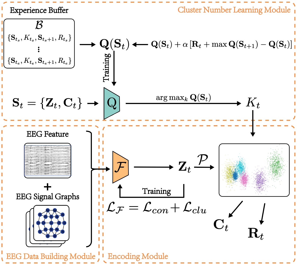
Overview of the ARLC-Net framework
1. Introduction
As the human lifespan progresses, interactions between different brain regions undergo significant transformations, reflecting dynamic changes in brain functional connectivity throughout neural development, maturation, and aging 1,2. Electroencephalography (EEG), a non-invasive neurophysiological monitoring technique with high temporal resolution, offers a unique window into tracking age-related neural dynamics 3. By decoding EEG signal variations, researchers can unravel micro-level evolutions of brain functions 4 and establish data-driven benchmarks for brain development and aging—foundations for personalized diagnostic tools and AI-based neurodevelopmental assessment software 5. Notably, accumulating neurophysiological evidence confirms that brain maturation and aging are characterized by discrete “critical periods” (e.g., infancy, adolescence, late adulthood) 6,7, where functional connectivity patterns undergo qualitative reorganizations, supporting the biological plausibility of age-based clustering.
Recent research on EEG and aging has advanced through multidimensional approaches. In the time-frequency domain, Morales and Bowers 5 developed a dynamic time-frequency analysis method, revealing a non-linear relationship between theta band energy and age in children and adolescents. Marek et al. 8 demonstrated that gamma oscillation trajectories in the anterior cingulate cortex serve as quantifiable markers for executive function maturation. In deep learning-based brain age prediction, Wong et al. 9 proposed a bi-directional long-short-term memory (Bi-LSTM) network to decode age-related neural patterns from resting-state EEG, while Li et al. 10 leveraged graph convolutional networks (GCNs) to capture non-linear neurodevelopmental trajectories for infant brain age estimation. In EEG-based clustering, Wang et al. 11 proposed a semi-supervised graph attention autoencoder (SGAAE-AC) that models inter-channel relationships via graph attention and integrates multi-objective optimization; however, in the same study, they also highlighted that EEG-based brain age clustering remains an understudied area.
Beyond EEG-specific work, unsupervised clustering methods for adaptive cluster number inference have been explored in broader fields, including nonparametric Bayesian approaches (e.g., Dirichlet-process mixtures 12, DP-means 13), growing neural gas 14, and autoencoder-based deep clustering 15. While these methods avoid predefined cluster numbers (\(K\)), they face critical limitations when applied to EEG data: (1) nonparametric Bayesian methods suffer from high computational complexity, making them infeasible for large-scale EEG datasets 12; (2) traditional adaptive clustering algorithms (e.g., DP-means) lack mechanisms to integrate EEG’s spatial-temporal structure and functional connectivity information 13. Additionally, most existing EEG-based age analysis methods rely on supervised regression or semi-supervised clustering 11,16, which depend on predefined age labels—limiting exploration of “natural grouping” patterns where chronological age diverges from brain age (e.g., premature aging, neurodegenerative diseases) 17. In contrast, unsupervised clustering can uncover intrinsic age-related functional connectivity patterns without label bias 18,19, yet their application to EEG age clustering remains sparse and constrained by the aforementioned limitations.
In the task of EEG-based brain age clustering, two core challenges persist:
-
・
Predefined cluster number dependency: Conventional clustering models (e.g., \(K\)-means) require manual specification of \(K\), a hyperparameter that directly governs clustering validity. For EEG data, over-fragmentation (excessive \(K\)) artificially splits biologically homogeneous neural patterns, while under-partitioning (insufficient \(K\)) merges neurodevelopmentally distinct age groups—obscuring critical transitions such as adolescence-to-adulthood. EEG’s high dimensionality, noise, and inter-subject variability further obscure the “natural” \(K\), making manual tuning unreliable 20.
-
・
Mismatch between general clustering methods and EEG characteristics: Existing adaptive clustering methods (e.g., Dirichlet-process mixtures 12, growing neural gas 14) are not tailored to EEG’s unique properties (e.g., phase synchronization-based functional connectivity, spectral power dynamics), leading to poor clustering cohesion and biological interpretability.
To address these challenges, we propose ARLC-Net, an adaptive representation learning framework for EEG-based brain age clustering. This study makes the following key contributions:
-
・
EEG-tailored adaptive clustering optimization: We design an adaptive clustering optimization (ACO) module that formulates cluster number inference as a Markov decision process (MDP). Unlike general adaptive clustering methods (e.g., DP-means 13, autoencoder-based approaches 15), the ACO module integrates reinforcement learning (RL) with EEG-specific constraints (e.g., phase synchronization, spectral power separation) via a clustering-driven reward function. This enables joint optimization of cluster number estimation and representation learning, eliminating reliance on predefined \(K\) while aligning clusters with biological age-related patterns.
-
・
Biologically grounded unsupervised learning: ARLC-Net leverages EEG’s spatial-temporal structure (e.g., phase locking value-based adjacency matrices) to learn age-relevant representations, addressing the limitation of general adaptive clustering methods in capturing EEG-specific functional connectivity.
2. Methods
2.1. Symbols and Problem Definition
To address the large number of symbols used in this paper, Table 1 a summary of these symbols.
| Notation | Meaning |
| \({X\in \mathbb{R}^{N\times d}}\) | Original feature matrix |
| \(A\in \mathbb{R}^{N\times N}\) | Original adjacency matrix |
| \(Z_t\in \mathbb{R}^{N\times d}\) | Node state at epoch \(t\) |
| \(C_t\in \mathbb{R}^{K \times d}\) | Cluster state at epoch \(t\) |
| \(K_t\in \mathbb{R}\) | Learned cluster number at epoch \(t\) |
| \(S_t=(Z_t,C_t)\) | State at epoch \(t\) |
| \(R_t\in \mathbb{R}\) | Reward at epoch \(t\) |
| \({\mathcal{F}}\) | Sample encoder network |
| \(Q\) | Quality network |
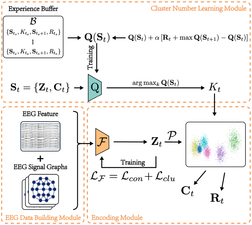
Fig. 1. The ARLC-Net. The EEG feature matrix and EEG adjacency matrix as input, is processed by the encoder \(\mathcal{F}\) in an unsupervised learning framework. Meanwhile, the quality network \(Q\) is designed to estimate cluster numbers (actions) under state \({S}_{{t}}\). Additionally, a clustering-specific reward \({R}_{{t}}\) is introduced to improve the cohesion within clusters while enhancing the separation between distinct clusters. The quality network is optimized by maximizing \({Q(S_t)}\) using the experience replay buffer \(C\).
2.2. Overall Framework of the Proposed Model
This section presents a detailed description of the adaptive representation learning clustering network (ARLC-Net). The ARLC-Net framework consists of three core modules: a EEG data building module, an encoder module, and a clustering number learning module. The overall framework is demonstrated in Fig. 1.
2.2.1. EEG Data Building Module
In this module, we employ the raw EEG feature data along with a preconstructed EEG graph structure as input to the encoder.
Raw EEG feature data consist of original time-domain signals collected from multiple electrodes. The EEG data are represented as \({X}\mathsf{\in}{\mathbb{R}}^{{N}\times{D}}\), where \(N\) denotes the number of EEG channels and \(D\) denotes the number of sampling points. Each signal \(x_i(t)\) corresponds to the EEG recording from electrode \(i\) at time point \(t\).
The other input is an EEG adjacency matrix \(A\in \mathbb{R}^{N\times N}\), constructed from 21 electrode channels arranged according to the international 10-20 system. Each element \(A_{ij}\) of the adjacency matrix is computed based on the phase locking value (PLV), which quantifies the synchronization between two electrode signals. The PLV matrix captures functional connectivity between electrodes and is computed as:
Here, \(A_{ij}\) denotes the PLV between electrodes \(i\) and \(j\), representing the degree of phase synchronization between their respective EEG signals. A value closer to 1 indicates stronger synchronization and thus a higher degree of functional connectivity. \(x_i(t)\) and \(x_j(t)\) are the time-domain EEG signals recorded from electrodes \(i\) and \(j\) at time \(t\), respectively. \(\|x_i(t)\|\) and \(\|x_j(t)\|\) denote the signal norms, which are used to normalize the amplitude of the signals to eliminate scale differences. \(T\) is the total number of time points, generally corresponding to the EEG signal’s recording duration.
This adjacency matrix describes the functional connection structure between electrodes and provides spatial dependency information for downstream feature extraction.
2.2.2. Encoder Module
The encoder \(\mathcal{F}\) encodes the nodes into embedding representations \(Z\in \mathbb{R}^{N\times d}\), as follows:
Specifically, the encoder loss \(\mathcal{L}_{\mathcal{F}}\) consists of a contrastive loss \(\mathcal{L}_{\mathrm{con}}\) and a clustering loss \(\mathcal{L}_{\mathrm{clu}}\), where the contrastive loss is defined as:
By minimizing \(\mathcal{L}_{\mathrm{con}}\), we can bring the representations of the same sample closer in different views and push away other negative samples.
To compute the clustering-guided loss \(\mathcal{L}_{\mathrm{clu}}\), we first obtain the cluster center matrix. The cluster center matrix, denoted as \(C\in {\mathbb{R}}^{K\times d}\), is computed by averaging the node embeddings \({Z}_{i}\) that belong to the same cluster, where \(K\) is the current number of clusters and \(C_j\in {\mathbb{R}}^d\) represents the center vector of the \(j\)-th cluster. The clustering-guided loss \(\mathcal{L}_{\mathrm{clu}}\) is then defined based on the distances between node embeddings and these cluster centers:
Finally, the total loss function of the encoder is defined as:
After the encoding process, the embedding representation \(Z\) is input to the clustering algorithm \(\mathcal{P}\), which generates the clustering results, including the cluster center matrix \(C\) and the cluster assignment matrix \(P\):
2.2.3. Cluster Number Learning Module
In this section, we introduce a cluster number learning module based on ACO. The process of determining the number of clusters in ACO is formulated as a Markov decision process (MDP). ACO module comprises four core components: states, actions, rewards, and transitions. The detailed design is as follows:
State.
At the \({t}\)-th iteration, the state \(S_{t}\) is jointly constructed from the node and cluster representations. Its definition is as follows:
Action.
The action \(A_t\) is composed of discrete and continuous actions, where the discrete actions adjust the number of clusters, and the continuous actions refine the positions of the cluster centers.
Discrete Action (\(A_{global}\)): Used to globally adjust the number of clusters \(K_t\), with the objective of learning an evaluation network \(Q\), which estimates the expected cumulative reward for selecting \(K_t\) given the state \(S_t\). The training process employs an experience replay strategy, collecting tuples of state, action, next state, and reward into an experience buffer \(\mathcal{B}\), as shown below:
Continuous Action (\(A_{local}\)): Refines the position of each cluster by optimizing the cluster centers \(C_t\). The action set is defined as \(A_{local}=\{\Delta{C_{1}},\Delta{C_{2}},\ldots,\Delta{C_{K_{t}}}\}\), with the update rule for each cluster center as:
Transition.
During training, as the number of epochs increases, the encoder is optimized by minimizing the encoder loss \(\mathcal{L}_{\mathcal{F}}\). This process transitions the state from \(S_{t}=\{Z_{t},C_{t}\}\) to \(S_{t+1}=\{Z_{t+1},C_{t+1}\}\).
Reward.
In order to dynamically optimize both the number of clusters and the clustering quality, we designed a reward function, which is defined as follows:
This reward function does not rely on age labels and is based solely on a general internal clustering evaluation metric derived from the structural properties of the learned embeddings. As such, it exhibits strong cross-dataset adaptability. Experimental results confirm that our approach effectively optimizes the clustering structure on both the TUAB and CHBMP datasets, which differ in age distribution (see Table 2).
| Method | Source | TUAB | CHBMP | ||||
| SCI | CHI | DBI | SCI | CHI | DBI | ||
| DMGC (2024) 22 | TCSS | 0.58\(\pm\)0.13 | 533.45\(\pm\)2.2 | 0.79\(\pm\)0.04 | 0.55\(\pm\)0.11 | 520.10\(\pm\)1.5 | 0.81\(\pm\)0.03 |
| CVGAE (2024) 23 | PR | 0.28\(\pm\)0.04 | 460.11\(\pm\)1.1 | 1.89\(\pm\)0.16 | 0.30\(\pm\)0.06 | 445.25\(\pm\)2.8 | 1.95\(\pm\)0.05 |
| ACD-EEG (2024) 24 | BSPC | 0.57\(\pm\)0.03 | 554.16\(\pm\)1.8 | 0.91\(\pm\)0.04 | 0.63\(\pm\)0.13 | 579.74\(\pm\)1.69 | 0.91\(\pm\)0.14 |
| EGRC-Net (2023) 25 | TIP | 0.24\(\pm\)0.02 | 352.12\(\pm\)2.5 | 1.34\(\pm\)0.05 | 0.26\(\pm\)0.04 | 360.4\(\pm\)3.85 | 1.40\(\pm\)0.05 |
| DmoN (2023) 26 | JMLR | 0.59\(\pm\)0.02 | 587.42\(\pm\)1.0 | 0.69\(\pm\)0.03 | 0.61\(\pm\)0.05 | 583.30\(\pm\)2.2 | 0.67\(\pm\)0.03 |
| SCGC (2023) 27 | TNNSL | 0.39\(\pm\)0.11 | 471.14\(\pm\)3.5 | 2.33\(\pm\)0.07 | 0.42\(\pm\)0.03 | 480.20\(\pm\)2.7 | 2.25\(\pm\)0.06 |
| ssvEEGc (2023) 28 | BSPC | 0.42\(\pm\)0.13 | 482.64\(\pm\)2.9 | 1.29\(\pm\)0.05 | 0.51\(\pm\)0.13 | 469.7\(\pm\)2.11 | 1.24\(\pm\)0.05 |
| R-GAE (2022) 29 | TKDE | 0.41\(\pm\)0.01 | 458.39\(\pm\)2.3 | 1.72\(\pm\)0.06 | 0.43\(\pm\)0.07 | 465.50\(\pm\)1.4 | 1.75\(\pm\)0.06 |
| DCRN (2022) 30 | AAAI | 0.54\(\pm\)0.12 | 520.78\(\pm\)2.6 | 0.92\(\pm\)0.04 | 0.56\(\pm\)0.03 | 530.45\(\pm\)1.8 | 0.88\(\pm\)0.04 |
| SS-EEG (2022) 31 | IEEE | 0.41\(\pm\)0.03 | 491.25\(\pm\)2.0 | 0.74\(\pm\)0.04 | 0.51\(\pm\)0.06 | 493.63\(\pm\)2.2 | 1.25\(\pm\)0.05 |
| AGCN (2021) 32 | ACM | 0.35\(\pm\)0.01 | 374.85\(\pm\)2.2 | 0.97\(\pm\)0.03 | 0.38\(\pm\)0.05 | 390.20\(\pm\)1.5 | 0.94\(\pm\)0.05 |
| CCG-EEG (2021) 33 | IEEE | 0.36\(\pm\)0.02 | 463.75\(\pm\)3.1 | 1.56\(\pm\)0.06 | 0.39\(\pm\)0.03 | 423.67\(\pm\)2.3 | 1.63\(\pm\)0.06 |
| ARGA (2019) 34 | IJCAI | 0.46\(\pm\)0.09 | 512.67\(\pm\)2.9 | 2.04\(\pm\)0.07 | 0.48\(\pm\)0.08 | 505.80\(\pm\)2.0 | 2.10\(\pm\)0.07 |
| ARLC-Net | Ours | 0.62\(\pm\)0.02 | 576.54\(\pm\)1.8 | 0.65\(\pm\)0.03 | 0.64\(\pm\)0.02 | 586.20\(\pm\)1.9 | 0.63\(\pm\)0.01 |
3. Experiments
3.1. Data
3.1.1. TUAB EEG Data
The EEG dataset of Temple University Hospital (TUH) 35 is one of the largest and most comprehensive publicly available EEG datasets currently available. One of its subsets, TUAB, is helpful for conducting research on automatic EEG diagnostic assessment. This dataset covers both male and female patients, with an age ranging from 7 days after birth to 96 years old. The sampling rate is 256 Hz, and the electrode channels adopt the international standard 10-20 system. The dataset contains 1,529 normal EEG recordings and 1,190 abnormal EEG recordings. The TUAB data can be accessed and used through the following link: https://isip.piconepress.com/projects/tuh_eeg/.
3.1.2. CHBMP EEG Data
The Cuban Human Brain Atlas Project (CHBMP) 36 provides a comprehensive multimodal EEG dataset, which includes recordings from individuals of all ages ranging from young to middle-aged in the general population. The CHBMP dataset studies healthy participants without significant medical history, and 253 healthy individuals from the CHBMP dataset contributed their resting-state EEG data for this study. This sample includes 89 females and 164 males, with an age range of 7–68 years. The resting-state EEG data were recorded using a high-density system with 64 to 120 electrode channels, with each recording lasting at least 30 minutes, including conditions such as eyes closed, eyes open, and hyperventilation. The CHBMP data can be accessed and used through the following link: https://chbmp-open.loris.ca.
3.1.3. Preprocessing of EEG Data
Given the significant inter-subject variability and inherent noise (e.g., ocular, muscular, cardiac artifacts) in EEG signals, we implemented a rigorous multi-stage preprocessing pipeline prior to feature extraction. This process ensures data consistency, enhances signal quality, and mitigates the impact of non-neural noise, thereby providing robust inputs for subsequent modeling.
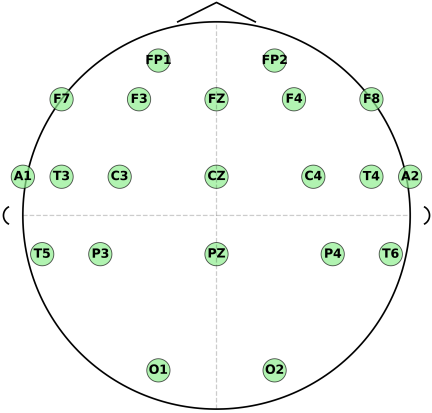
Fig. 2. Brain area distribution map.
-
・
Channel Selection and Resampling: To ensure spatial and temporal consistency across all samples, EEG recordings were first standardized. We selected 21 electrodes (detailed selection shown in Fig. 2) common across recordings according to the international 10-20 system. All data were uniformly resampled to a frequency of 256 Hz.
-
・
Band-pass Filtering: A zero-phase (0.5–45 Hz) band-pass finite impulse response (FIR) filter was applied. This step removes low-frequency drift (\(<0.5\) Hz), power-line interference (\(\sim\)50/60 Hz), and high-frequency muscle artifacts (\(>45\) Hz), preserving the neurophysiologically relevant oscillatory content within the delta, theta, alpha, and beta bands.
-
・
Amplitude Normalization: To minimize the influence of individual differences in signal amplitude (e.g., due to scalp conductivity or electrode impedance), each channel’s time series was standardized using \(z\)-score normalization \((x^{\prime}=(x-\mu)/\sigma)\), where \(\mu\) and \(\sigma\) are the mean and standard deviation of the signal per channel per recording.
This preprocessing ultimately ensured data quality and consistency. The TUAB and CHBMP datasets were then split into training, validation, and test sets in a \(6:2:2\) ratio to ensure that the data sources for model training, validation, and testing did not overlap.
3.2. Evaluation Metrics
The evaluation methods for clustering results can generally be divided into external evaluation and internal evaluation.
External evaluation requires known true class labels of the samples, and the evaluation is based on the consistency between the clustering results and the true labels. Commonly used metrics include accuracy (ACC), normalized mutual information (NMI), and adjusted rand index (ARI).
Internal evaluation does not rely on any external information but instead evaluates the clustering results based on the structural properties of the clusters and the distribution characteristics of the samples themselves. The core idea is to measure intra-cluster compactness and inter-cluster separation, which is suitable for unlabeled data.
However, the calculation of traditional supervised metrics (ACC, NMI, ARI) is based on the premise that there exists a ground truth label set y-true, against which the clustering result (predicted labels y-pred) is compared. Since this study focuses on the clustering task of unlabeled EEG data, employing these traditional supervised metrics (ACC, NMI, ARI) is not applicable. Therefore, we selected the following three classical internal evaluation metrics: silhouette coefficient index (SCI) 37, Calinski–Harabasz index (CHI) 38, and Davies–Bouldin index (DBI) 39, which respectively quantify clustering quality from three orthogonal perspectives: sample-level compactness, global variance explained, and the worst inter-cluster confusion. This approach avoids the limitations of a single metric and provides a robust evaluation for unsupervised EEG clustering.
3.3. Experimental Results
Given the current lack of algorithms specifically designed for EEG signal age clustering tasks, to comprehensively assess the performance of our proposed ARLC-Net method, we compared it with several state-of-the-art clustering methods from two perspectives: general graph clustering and EEG-specific clustering. For the former, we selected nine representative deep graph clustering methods that, while not designed for EEG age clustering, have demonstrated strong performance on graph-structured data and serve as widely recognized benchmarks in the field. These include three major categories: reconstruction-based methods (DMGC, EGRC-Net, DmoN, R-GAE, AGCN), adversarial methods (ARGA), and contrastive methods (DCRN, SCGC, CVGAE).
For the latter, we introduced four EEG-specific clustering methods that explicitly model temporal or spectral features of EEG signals. We briefly outline their core calculation mechanisms below:
-
・
Electroencephalogram Signal Clustering with Convex Cooperative Games (CCG-EEG): This method maps the clustering task to a convex cooperative game where EEG trials act as players. The calculation proceeds in three steps: (i) it first computes a modified cross-correlation (LotNCC) to measure pairwise similarity between EEG trials; (ii) it then calculates the Shapley value for each trial using a closed-form formula derived from the convex game property, which quantifies the marginal contribution of each trial to the coalition; (iii) finally, it identifies the trial with the highest Shapley value as the cluster center and assigns remaining trials to this cluster if their similarity to the center exceeds a predefined threshold \(\delta\). This process iterates until all trials are clustered.
-
・
Semi-Supervised EEG Clustering with Multiple Constraints (SS-EEG): This approach formulates semi-supervised clustering as a graph embedding problem with an optimization objective function integrating multiple constraints. The calculation involves minimizing a unified loss function comprising: (i) label-transformed connectivity constraints, which enforce connections for same-label pairs and disconnections for different-label pairs via the graph Laplacian; (ii) a compactness-and-scatter constraint relaxed into a fairness-constrained Normalized Cut (NCut) to balance intra-cluster compactness and inter-cluster scatter; and (iii) a fairness constraint to ensure balanced cluster sizes. The optimal pseudo-labels and adjacency matrix are solved iteratively using a gradient descent strategy until convergence to a local optimum.
-
・
An Efficient EEG Clustering Method Using Balance-Constrained Voting Mechanism (ssvEEGc): This method employs a simulated voting mechanism to assign unlabeled trials efficiently. The calculation for each unlabeled trial \(a\) involves: (i) computing the intra-cluster compactness (\(S_{in}\)) for each existing labeled cluster, defined as the average pairwise distance within the cluster; (ii) calculating a voting rate (\(R_{j}\)) , which is the proportion of labeled trials in cluster \(C_{j}\) whose distance to \(e_{u}\) is less than \(S_{in}\); (iii) determining a balance factor (\(B_{j}\)) based on the current cluster size relative to the total data; and (iv) assigning \(e_{u}\) to the cluster \(C_{j}\) that maximizes the weighted score \(\sigma_{j}=\alpha R_{j}+(1-\alpha)B_{j}\), thereby ensuring both similarity and cluster balance.
-
・
Adaptive Channel-Weight Dual-Constrained Semi-Supervised EEG Clustering (ACD-EEG): This method enhances semi-supervised clustering by incorporating channel importance. Its calculation follows an alternating iterative optimization of four variables: (i) feature extraction: it first applies improved adaptive neighborhood minmax projections (I-ANMMP) to learn a subspace that minimizes intra-class and maximizes inter-class distances; (ii) channel weighting: it learns an optimal channel weight vector \({c}\) by minimizing the least squares error between the learned pseudo-adjacency matrix and the weighted sum of channel-wise similarity matrices; (iii) dual constraints: it integrates connectivity constraints (for labeled data) and neighborhood constraints (for spatial relationships) into the objective function; and (iv) pseudo-label learning: it updates pseudo-labels and the classifier via gradient descent to minimize cross-entropy loss and regularized least-square error simultaneously.
To ensure a fair and meaningful comparison, we systematically adapted all benchmark methods to accommodate EEG-specific characteristics. For general graph clustering methods (including reconstruction-based methods like DMGC, EGRC-Net, DmoN, R-GAE, AGCN; adversarial methods like ARGA; and contrastive methods like DCRN, SCGC, CVGAE), the adaptation focused on integrating EEG’s spatial topology and temporal-spectral content. Specifically, each EEG channel was treated as a node in the graph, with the adjacency matrix constructed using the phase locking value (PLV) derived from the raw time-series signals (as defined in Eq. (1)), thereby encoding functional connectivity between channels. To incorporate temporal information, we transformed the raw time-domain signals for each channel into node feature vectors by extracting power spectral density features across the \(\delta\), \(\theta\), \(\alpha\), and \(\beta\) frequency bands. This process effectively captures the spectral dynamics of EEG, which are critical for age-related analysis. By combining the PLV-based adjacency matrix (spatial) with frequency-band power features (temporal-spectral), these general graph clustering models were enabled to process EEG data in a manner consistent with the proposed ARLC-Net. For EEG-specific clustering methods (e.g., CCG-EEG, SS-EEG, ssvEEGC, ACD-EEG), we followed their original designs which inherently incorporate spatial and temporal mechanisms; only the preprocessing and evaluation protocols were unified to ensure fairness.
To holistically assess clustering quality without ground-truth labels, we employ three complementary internal validation metrics: SCI (higher is better), CHI (higher is better), and DBI (lower is better). Since no single metric can fully capture partition quality, our claim of superiority is based on a deliberate assessment strategy that prioritizes substantial and balanced improvement across these metrics. Specifically, we focus on the relative percentage improvement (or reduction) of ARLC-Net against the strongest baseline for each dataset, as this quantifies the practical significance of performance gains beyond marginal differences.
The complete quantitative results are presented in the Table 2. On the TUAB dataset, ARLC-Net achieves the best scores in SCI (0.62) and DBI (0.65). Compared to the second-best method (DmoN, SCI: 0.59, DBI: 0.69), this represents a \(+5.1\%\) improvement in SCI and a \(-5.8\%\) improvement (reduction) in DBI. While DmoN attains a slightly higher CHI (587.42 vs. ARLC-Net’s 576.54), the relative difference is only \(-1.9\%\). Crucially, the magnitude of improvement in SCI and DBI far outweighs this marginal shortfall in CHI, demonstrating ARLC-Net’s superior ability to enhance sample-level compactness and worst-case cluster separation. On the CHBMP dataset, ARLC-Net outperforms all baselines across all three metrics, achieving the highest SCI (0.64) and CHI (586.20), and the lowest DBI (0.63), which further confirms its robustness and generalizability.
These results collectively demonstrate ARLC-Net’s superior performance in uncovering latent relationships between EEG signals and age, validated by a consistent pattern of significant, balanced gains across key evaluation dimensions.
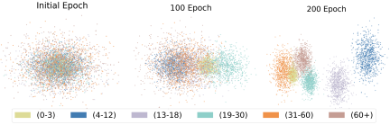
Fig. 3. Evolution of clustering performance of the model.
From a data-driven perspective, the TUAB dataset (age range: 7 days to 96 years) was optimally partitioned into six distinct clusters exhibiting high intra-cluster cohesion and inter-cluster separation. These clusters correspond to six statistically significant age groups: 0–3, 4–12, 13–18, 19–30, 31–60, and \(>60\) years (see Fig. 3). Similarly, the CHBMP dataset (age range: 7–68 years) was partitioned into five well-separated clusters corresponding to age groups: 7–12, 13–19, 20–32, 33–62, and \(>62\) years.
Although ARLC-Net identified six clusters in TUAB and five in CHBMP, significant consistency was observed. The average boundary error in overlapping age ranges (7–68 years) was merely 1.25 years (relative error \(<2\%\)). This divergence stems from fundamental differences in age coverage—TUAB includes critical infant developmental stages (0–6 years) absent in CHBMP. ANOVA validation (\(p<0.001\), \(\eta^{2}>0.78\)) confirmed statistically significant inter-group differences and intra-group cohesion (silhouette score \(>0.6\)) in both partitions. Boundary alignments—childhood/adolescence (12 years), adolescence/young adulthood (18 vs. 19 years), young/middle adulthood (30 vs. 32 years), and middle/late adulthood (60 vs. 62 years)—all conform to established neurodevelopmental characteristics. This evidences ARLC-Net’s ability to adapt to data distributions while maintaining biological plausibility for robust age clustering.
3.4. Validation and Robust Test
To validate the effectiveness of the proposed cluster number learning module, we employed both the ARLC-Net method and the classic \(K\)-means method 40 to estimate the optimal number of clusters for the TUAB dataset (abnormal dataset). The within–cluster sum of squares (WSS) was used as an evaluation metric, which is defined as:
Specifically, the ARLC-Net module employs reinforcement learning to iteratively calculate the WSS for each cluster number until it identifies the optimal cluster and calculates the WSS for this optimal cluster, as illustrated in Fig. 4(a). On the other hand, Fig. 4(b) shows the classic \(K\)-means method, which tests cluster numbers from 2 to 9 and calculates their corresponding WSS. Based on the training results shown in Fig. 4, we draw the following conclusions:
Although the TUAB dataset (abnormal dataset) contains some anomalies, our model can still identify the best cluster number from a data-driven perspective, whereas the classic \(K\)-means method fails to find any plateau due to irregular WSS trends, leading to the failure of elbow method.
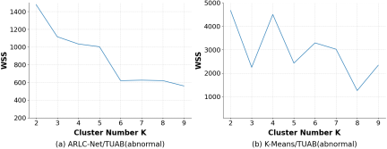
Fig. 4. The ARLC-Net method and the \(K\)-means method each search for the optimal number of clusters on the TUAB dataset (abnormal dataset).
This study utilizes two EEG datasets: TUAB (normal EEG data, age range: 7 days to 96 years) and CHBMP (age range: 7–68 years). Given that CHBMP lacks coverage of early infancy (0–6 years) and advanced aging (\(>68\) years), all cross-age analyses of EEG spatial distribution patterns were exclusively performed on the TUAB normal dataset. This selection ensures comprehensive characterization of dynamic neural trajectories across the full neurodevelopmental continuum, capturing critical spatial-topological transitions during infant synaptogenesis, adolescent network reorganization, and senescent functional decline.
3.5. Robustness and Generalization Analysis
To comprehensively evaluate the performance of ARLC-Net when facing common challenges of real-world EEG data, the experimental results (see Table 3) clearly demonstrate the model’s performance under various data conditions.
| Condition | Parameter | TUAB | CHBMP | ||||
| SCI | CHI | DBI | SCI | CHI | DBI | ||
| ARLC-Net | 256 Hz, 21 ch, filtered, normalized | 0.62 | 576.54 | 0.65 | 0.64 | 586.20 | 0.63 |
| Additive noise | Gaussian noise, \(\mathrm{SNR} = 20\) dB | 0.61 | 560.12 | 0.70 | 0.62 | 570.25 | 0.68 |
| Gaussian noise, \(\mathrm{SNR} = 10\) dB | 0.53 | 512.34 | 0.85 | 0.55 | 522.47 | 0.82 | |
| Gaussian noise, \(\mathrm{SNR} = 5\) dB | 0.41 | 445.67 | 1.25 | 0.43 | 455.80 | 1.20 | |
| Sampling rate | Downsampled to 128 Hz | 0.61 | 568.90 | 0.67 | 0.63 | 578.35 | 0.65 |
| Downsampled to 64 Hz | 0.55 | 525.45 | 0.80 | 0.57 | 535.60 | 0.78 | |
| Upsampled to 512 Hz | 0.62 | 575.80 | 0.66 | 0.64 | 585.45 | 0.64 | |
| Different montage | 30 channels (10-10 system) | 0.61 | 571.49 | 0.64 | 0.63 | 579.43 | 0.62 |
| Ablated preprocessing | No band-pass filtering | 0.48 | 475.20 | 0.95 | 0.50 | 485.35 | 0.92 |
| No amplitude normalization | 0.45 | 460.15 | 1.05 | 0.47 | 470.30 | 1.02 | |
| No preprocessing (raw signal) | 0.32 | 395.60 | 1.50 | 0.34 | 405.75 | 1.45 | |
Robustness to Noise: We simulated data quality issues by adding Gaussian noise with different signal-to-noise ratios (SNR) to the EEG signals. Under mild noise conditions (\(\mathrm{SNR} = 20\) dB), the model’s performance metrics (SCI, CHI, DBI) on both TUAB and CHBMP showed only a slight decrease compared to the baseline, which is virtually negligible. Even under moderate noise (\(\mathrm{SNR} = 10\) dB), the model could still maintain most of the clustering structure (\(\mathrm{SCI} = 0.53\)), indicating a certain tolerance to common background noise. However, performance declined significantly under extreme noise (\(\mathrm{SNR} = 5\) dB), which is as expected and further emphasizes the necessity of appropriate cleaning for high-noise data before analysis.
Adaptability to Different Sampling Rates: To test whether the model is constrained by specific acquisition protocols, we evaluated its performance under different sampling rates. When the data were downsampled from 256 Hz to 128 Hz, the model’s performance remained almost on par with the baseline, proving that ARLC-Net remains effective at conventional clinical sampling rates. A noticeable performance drop occurred when downsampled to 64 Hz, likely due to the lower temporal resolution affecting the accurate estimation of phase synchronization (PLV). After upsampling the data to 512 Hz, performance aligned with the baseline, indicating the model’s compatibility with higher sampling rate data.
Robustness to Changes in Electrode Configuration (Montage): We compared the standard 21-channel (10-20 system, the electrode configuration used by ARLC-Net) and the 30-channel (10-10 system) and re-trained the model. The results showed that with the 30-channel of the 10-10 system, the spatial sampling density increased, but the performance of the model even decreased compared to the 21 electrode channels of the 10-20 system. Moreover, the 10-10 system used more channels and consumed more computing resources, which further proved that the 21 electrodes of the 10-20 system were sufficient to capture the key age-related spatial patterns.
Dependency Analysis on Preprocessing Steps: By progressively ablating preprocessing steps, we directly evaluated ARLC-Net’s dependency on specific processing pipelines. When band-pass filtering was removed, performance declined significantly, demonstrating that filtering is crucial for removing high-frequency noise and low-frequency drift. Removing amplitude normalization led to a further performance drop, suggesting that inter-individual amplitude differences may become confounding factors. Performance was poorest with completely unprocessed (raw) signals, confirming that standardized preprocessing is indispensable for functional connectivity-based EEG analysis. Nonetheless, ARLC-Net could still output meaningful clustering results when some preprocessing steps were missing, demonstrating a certain degree of fault tolerance.
Comprehensive Conclusion: The above experimental results indicate that ARLC-Net exhibits good robustness within reasonable ranges of real-world data variability (such as mild noise, common sampling rate changes, different electrode configurations). The model does not rely on a single, strict preprocessing pipeline, but its optimal performance does require adherence to basic EEG processing norms (such as filtering and normalization).
3.6. Parameter Sensitivity Analysis of the ACO Module
To ensure the robustness of the ACO module within ARLC-Net and clarify the impact of its core parameters on final performance, this section conducts a systematic sensitivity analysis of the key hyperparameters of the ACO module. We focus on the following four categories of parameters: learning rate (\(\alpha\)), buffer capacity, sampling strategy, and \(\varepsilon\)-greedy exploration rate (\(\varepsilon\)). The analysis aims to evaluate how these parameters affect: 1) the learning quality of the \(Q\)-network (measured by the state value \(Q(S_t)\), higher is better); 2) the final clustering quality (evaluated by SCI, CHI, DBI); 3) the convergence speed of the algorithm (measured by the number of training epochs required to reach stable clustering). All experiments were conducted on the TUAB and CHBMP datasets, changing only one target parameter at a time while keeping the others at their preliminary validated default values.
Learning Rate (\(\alpha\)): Controls the step size for updating the \(Q\)-network weights based on temporal difference error. Excessively high \(\alpha\) may lead to oscillating and unstable \(Q\)-value estimates, hindering convergence; excessively low \(\alpha\) makes the learning process slow and inefficient.
Experience Replay Buffer Capacity: The maximum length of the queue storing past state transition experiences (\(\mathcal{B}={S_t,K_t,S_{t+1},R_t}\)). Too small a capacity may result in high sample correlation and rapid forgetting of early experiences; too large a capacity may introduce too many stale experiences, slowing down the learning process.
Sampling Strategy: The method for sampling experience batches from the buffer. Uniform random sampling serves as the baseline strategy; prioritized experience replay (PER) assigns different priorities to samples based on the magnitude of temporal difference error, with samples having larger errors having a higher probability of being selected, aiming to learn from “difficult” experiences more efficiently.
\(\varepsilon\)-Greedy Exploration Rate (\(\varepsilon\)): During training, with probability \(\varepsilon\), a random action (adjusting the cluster number) is chosen, and with probability \(1-\varepsilon\), the action currently deemed optimal by the \(Q\)-network is chosen. A higher \(\varepsilon\) encourages exploring more possible cluster numbers but may delay convergence; a lower \(\varepsilon\) favors exploiting current knowledge but may lead to getting stuck in a local optimum.
| Parameter | Tested value | TUAB | CHBMP | Selected | ||||||||
| SCI | CHI | DBI | \(Q(S_t)\) | Epochs | SCI | CHI | DBI | \(Q(S_t)\) | Epochs | |||
| Learning rate (\(\boldsymbol{\alpha}\)) | 0.001 | 0.59 | 556.12 | 0.81 | 0.75 | 85 | 0.62 | 576.76 | 0.93 | 0.77 | 80 | \(✓\) |
| 0.01 | 0.63 | 587.66 | 0.66 | 0.82 | 52 | 0.65 | 589.36 | 0.66 | 0.91 | 50 | ||
| 0.1 | 0.57 | 554.37 | 0.93 | 0.69 | 30 | 0.61 | 559.16 | 0.87 | 0.72 | 28 | ||
| Buffer capacity | 50 | 0.39 | 496.14 | 1.24 | 0.66 | 35 | 0.42 | 506.12 | 1.06 | 0.71 | 38 | \(✓\) |
| 100 | 0.60 | 556.83 | 0.72 | 0.79 | 55 | 0.62 | 567.49 | 0.69 | 0.74 | 58 | ||
| 150 | 0.46 | 536.19 | 0.98 | 0.72 | 90 | 0.53 | 543.85 | 0.84 | 0.73 | 88 | ||
| Sampling strategy |
Uniform random sampling |
0.42 | 492.26 | 1.09 | 0.63 | 68 | 0.51 | 512.89 | 1.12 | 0.63 | 72 | \(✓\) |
| Prioritized experience replay (PER) | 0.61 | 559.45 | 0.73 | 0.76 | 45 | 0.69 | 554.78 | 0.69 | 0.76 | 42 | ||
| Exploration rate (\(\boldsymbol{\varepsilon}\)) | 0.1 | 0.46 | 540.15 | 0.89 | 0.69 | 48 | 0.50 | 539.62 | 0.79 | 0.72 | 46 | \(✓\) |
| 0.3 | 0.51 | 532.19 | 0.72 | 0.66 | 55 | 0.49 | 543.16 | 0.80 | 0.69 | 58 | ||
| 0.5 | 0.63 | 592.78 | 0.63 | 0.89 | 54 | 0.65 | 589.17 | 0.66 | 0.82 | 52 | ||
| 0.7 | 0.54 | 543.89 | 0.92 | 0.73 | 72 | 0.57 | 529.46 | 0.73 | 0.72 | 70 | ||
Table 4 shows the results of the sensitivity analysis under different parameter configurations. Each row represents the performance when changing one parameter value. The experiments were performed on both TUAB and CHBMP datasets. The results demonstrate that:
-
・
Learning Rate (\(\alpha\)): \(\alpha=0.001\) converges slowly due to excessively small update steps (TUAB: 85 epochs, CHBMP: 80 epochs), with final SCI slightly below the optimal value. \(\alpha=0.01\) achieves the best balance between convergence speed (about 50 epochs) and clustering quality (SCI \(\approx 0.63/0.65\)), with low \(Q\)-value variance and stable training. \(\alpha=0.1\) converges quickly (about 30 epochs) but exhibits significant \(Q\)-value oscillations, leading to degraded clustering performance (SCI drops to \(0.57/0.61\)).
-
・
Experience Replay Buffer Capacity: When the capacity is 50, the buffer is too small, resulting in highly correlated samples and rapid overwriting of early experiences. Although the model quickly fits recent experiences (about 35 epochs), its generalization ability is poor, with SCI only \(0.39/0.42\). A capacity of 100 retains sufficiently diverse experiences while avoiding excessive stale samples, achieving reasonable convergence speed (about 55 epochs) and optimal clustering performance (SCI \(0.60/0.62\)). When the capacity is 150, performance degrades rather than improves because, as the encoder updates, the node representations \(Z_{t}\) and cluster centers \(C_{t}\) continuously evolve, and the state transitions stored early in the buffer gradually become mismatched with the current data distribution. An excessively large capacity introduces a large amount of “stale” experience, requiring the model to spend additional time (about 90 epochs) filtering out useful information, and it is ultimately still disturbed by stale samples, leading to a drop in SCI to \(0.46/0.53\) and an increase in DBI. This reveals that in a non-stationary state space, the buffer capacity must match the rate of state evolution, and larger is not always better.
-
・
Sampling Strategy: Uniform random sampling converges slowly (about 70 epochs) and yields relatively low \(Q\)-values because numerous simple samples dominate training, making it difficult to focus on “difficult” experiences with high TD error. PER, by assigning higher sampling weights to samples with larger TD errors, significantly accelerates convergence (about 45 epochs) while improving both \(Q\)-values and clustering quality, demonstrating its ability to utilize limited experience more efficiently.
-
・
\(\varepsilon\)-Greedy Exploration Rate (\(\varepsilon\)): \(\varepsilon=0.1\) leads to insufficient exploration, easily getting stuck in local optima; although convergence is relatively fast (about 48 epochs), performance is mediocre. \(\varepsilon=0.3\) strikes a balance slightly favoring exploitation, but convergence speed and performance are not optimal. \(\varepsilon=0.5\) achieves the best trade-off between exploration and exploitation, with moderate convergence speed (about 54 epochs) and leading clustering metrics across the board (SCI \(0.63/0.65\), DBI \(0.63/0.66\)). \(\varepsilon=0.7\) results in excessive exploration, wasting training steps on many invalid actions, delaying convergence to about 70 epochs, and ultimately impairing final performance.
In summary, the selected default parameters (\(\alpha=0.1\), buffer capacity 100, PER sampling, \(\varepsilon=0.5\)) are optimal not only in terms of clustering quality but also achieve the best balance between convergence speed and training stability, validating the robustness and effectiveness of the ACO module design.
3.7. Analysis of Brain Network Changes Across Six Age Groups
3.7.1. Analysis of EEG Frequency Band Power in Different Age Groups
In this study, based on the ARLC-Net model, we automatically divided the data from the normal TUAB dataset into six age groups with statistically significant differences (0–3 years old, 4–12 years old, 13–18 years old, 19–30 years old, 31–60 years old, and over 60 years old) as the reference. We then calculated the logarithmic average power spectrum and power spectrum density of the EEG data for each age group to quantify the spatial distribution of the power in different EEG frequency bands. We focused on the delta (0.5–4 Hz), theta (4–8 Hz), alpha (8–13 Hz), and beta (13–30 Hz) frequency bands.
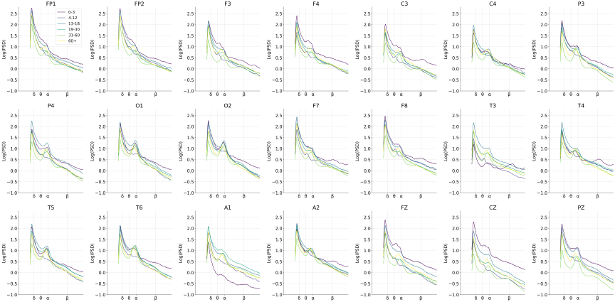
Fig. 5. The logarithmic mean spectrum of each frequency band for the six age groups.
It reveals the dynamic patterns of brain electrical activity across age. The overall trend aligns with theories of neurodevelopment and aging: slow-wave (delta/theta) power gradually decreases from high levels in infancy (0–3 years), while fast-wave (alpha/beta) power follows an inverted U-shaped trajectory, peaking in adolescence (13–18 years) and then gradually declining with age (see the Fig. 5). Specifically:
-
・
Age-related decline in delta/theta power: delta power peaks in the frontal lobe for the 0–3 year-old group (FP1: 2.208) and drops to 1.672 in the 60+ year-old group (a decrease of 24.3%). Theta power is high across the brain in the 0–3 year-old group but significantly decreases in the 60+ year-old group (a decrease of 44.9%).
-
・
Inverted U-shaped curve for alpha/beta: Occipital alpha power peaks at 13–18 years (O1: 1.173), decreasing to 0.785 in the 60+ year-old group (a decrease of 33.0%). Frontal beta power is higher in the 0–3 year-old group (F8: 0.512) and continuously decreases in adulthood (60+ years F8: 0.143, a decrease of 72.1%).
Key new findings include:
-
・
Rapid decline in frontal theta power: The average logarithmic power of theta waves in the frontal FP1 channel decreases by 44.9% from 1.403 in the 0–3 year-old group to 0.773 in the 60+ year-old group. This decline is significantly greater than that observed in the occipital O1 channel (0.979 \(\rightarrow\) 0.664, a decrease of 32.2%; difference of 12.7%) and the temporal T5 channel (0.916 \(\rightarrow\) 0.625, a decrease of 31.8%; difference of 13.1%). This region-specific decline in frontal theta power is consistent with longitudinal evidence showing a pronounced reduction of theta activity in frontal cortices with aging 41. Age-related alterations in frontal-midline theta have been linked to changes in cognitive maintenance 42, and theta oscillatory signatures of attentional control are known to change from middle to older age 43. Therefore, the pronounced frontal decline observed here suggests that the frontal-thalamic loop may be particularly sensitive to the aging process. This could provide a potential electrophysiological explanation for the well-documented decline in executive functions with age and offers a perspective that complements traditional models of aging.
-
・
Quantitative validation of slow-wave dominance in infants’ frontal lobes: This study finds that infants (0–3 years) exhibit a distinct “frontal dominance” pattern in slow-wave (primarily delta) activity, with power in other brain regions being significantly weaker. Specifically, the average logarithmic power of delta waves is 2.208 in the frontal lobe, compared to 0.765 in the anterior temporal lobe (a difference of \(-189\%\)), 1.704 in the primary sensory cortex (a difference of \(-29.6\%\)), and 1.701 in the occipital lobe (a difference of \(-29.8\%\)). It is worth noting that we also analyzed the alpha band (8–13 Hz) activity within this infant population, but did not observe a similar frontal lobe dominance pattern. In the 0 to 3-year-old age group, the alpha rhythm is not yet physiologically mature, and is typically weak or absent in the frontal lobe region. Usually, only a posterior dominance pattern emerges as the developmental process progresses. Therefore, unlike the robust and spatially specific delta wave findings, alpha activity is not a distinct indicator of frontal lobe maturation during infancy. This is why our quantitative verification mainly focused on the delta wave. This frontal predominance of slow-wave activity aligns with known features of early brain development. The development of crucial thalamocortical mechanisms, such as the coupling between slow oscillations and spindles, is an ongoing process throughout infancy 44. Furthermore, slow-wave activity in infancy has been established as a neurophysiological correlate of psychomotor development 45. Thus, our finding validates that frontal slow-wave (primarily delta) activity can serve as a sensitive indicator of frontal lobe maturation during early development. It highlights the spatially asynchronous nature of EEG development, prompting further investigation into the regional timelines of functional brain network specialization.
3.7.2. Analysis of the Changes in Dispersion Within the Network Across Different Age Groups
Figure 6 demonstrates the dispersion between different functional networks. Table 5 presents six functional networks and their anatomical significance. First, the weighted phase lag index method was used to calculate the functional connectivity strength between each pair of electrodes in specific frequency bands, resulting in a high-dimensional connectivity matrix. Principal component analysis was then applied to reduce the dimensionality of this matrix, mapping it into a three-dimensional gradient space, thereby extracting the main directions of variation in the connectivity patterns. To account for amplitude variations caused by age or individual differences, each gradient dimension was standardized. We then calculated the centroid positions of each functional network in this three-dimensional gradient space, which represent the spatial distribution of each network. Finally, the Euclidean distance between the centroids of different network pairs was calculated, quantifying the functional separation between the networks and revealing their independence and interrelationships. The overall trend aligns with neurodevelopment and aging theories, specifically in the following cases.
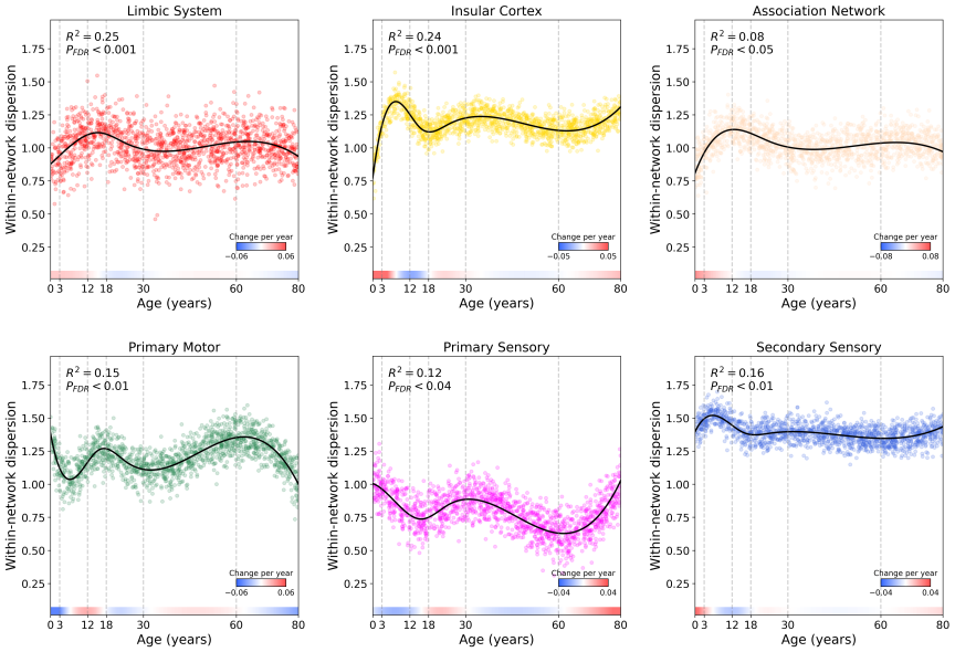
Fig. 6. Between-network dispersion across age groups.
| Network name | Core brain regions | Functional role | Corresponding EEG channels |
| Limbic | Amygdala | Memory | FP1, FP2 |
| Insular cortex | Insula | Emotional awareness | F7, F8 |
| Association network | Prefrontal cortex | Executive function | F3, FZ, F4 |
| Primary motor | Precentral gyrus | Movement execution | C3, CZ, C4 |
| Primary sensory | Postcentral gyrus | Basic sensory processing | P3, PZ, P4 |
| Secondary sensory | Surrounding primary areas | Complex sensory | T3, T4, T5, T6, O1, O2 |
During the developmental period (childhood to adolescence), the brain exhibits network segregation, meaning that the functional specificity between different networks increases, leading to higher dispersion. In adulthood (young to middle age), the brain enters a stage of functional integration, where different networks need to cooperate to support complex cognitive tasks. In older adulthood (60+ years), the brain shows functional dedifferentiation, where previously specialized connections weaken, and dispersion may decrease, serving as either a compensatory mechanism or a marker of aging.
In addition, Fig. 6 also reveals several key new findings:
-
・
Limbic-Association Network: U-shaped Trajectory Suggests Adolescent Emotional Integration and Midlife Cognitive Reorganization.
The dispersion of the limbic-association network increased from 1.05 in adolescence (13–18 years) to 1.42 in middle age (31–60 years), an increase of 35.2%. Notably, it reached its lowest value (1.05) during adolescence. Traditional theory suggests that the connection between the limbic system (emotion) and the prefrontal cortex (cognitive control) strengthens linearly with age. The new finding shows that during adolescence, this dispersion decreases instead of increasing, revealing an adolescent-specific “emotion-cognition coupling” mode. This may be due to dramatic hormonal changes and increased social demands, leading emotions to deeply engage in cognitive decision-making—consistent with adolescents’ emotional volatility and enhanced innovative thinking.
The strong rebound in dispersion in middle age (1.42) may reflect cognitive reorganization; individuals in midlife use more mature strategies to regulate emotions, manifested as renewed network separation to achieve more efficient and rational emotion-cognition balance. This aligns with the “expert brain” theory, which proposes that cognitive and emotional stability peak in middle age.
-
・
Secondary Sensory-Association Network: Peak Dispersion in Adolescence Reveals a Window for High-Level Sensory Integration.
The dispersion of the secondary sensory-association network reached 1.68 at 13–18 years, significantly higher than in childhood (4–12 years, 1.45) and young adulthood (19–30 years, peak before 1.74), with the adolescent value being particularly prominent.
This finding indicates that adolescence is a critical period for the deep integration of higher-order sensory information with the association cortex. During this time, the brain may prioritize resources to broadly connect complex sensory information (e.g., visual-spatial, auditory-linguistic) with high-level cognitive functions such as executive function and episodic memory, supporting the development of abstract thinking, complex learning, and social understanding.
Traditional research has focused more on the early development of the primary sensory cortex (which is considered relatively mature in childhood). This data suggests that the functional integration peak of higher-order sensory cortex is delayed until adolescence. This provides strong neuroscientific support for enhancing related cognitive training (e.g., spatial reasoning, artistic literacy) during adolescence.
-
・
Selective Functional Changes in Older Adulthood.
In older adulthood (60+ years), the dispersion of networks such as primary motor-primary sensory (1.55 vs. midlife 1.61, decreased 3.7%) and limbic-insular (1.58 vs. midlife 1.65, decreased 4.2%) showed slight but consistent declines. In contrast, the dispersion of the insular-association (1.62) and primary-secondary sensory (1.98) networks remained high or even increased slightly. This supports the view that the aging brain does not degenerate uniformly but rather undergoes selective functional changes.
The decline in dispersion in sensorimotor and emotional-interoceptive systems may reflect dedifferentiation in these basic functions—a reduction in network specificity, which could be a sign of functional decline or a compensatory strategy by the brain to maintain function (e.g., by recruiting more brain regions for the same task).
The maintained dispersion in the insular-association and sensory hierarchical networks suggests that higher-order cognitive integration and sensory information processing may be relatively well preserved in old age. This is crucial for maintaining cognitive quality of life and complex task-handling abilities in older adults.
This coexistence of changes reveals the complexity and heterogeneity of brain function in aging, indicating that research on aging requires fine-grained examination by network and system.
Figure 7 displays the dispersion values of each functional network across different age groups (7–12, 13–18, 19–30, 31–60 years) in the TUAB and CHBMP datasets side by side. Numerical analysis reveals that within the overlapping age range, TUAB and CHBMP exhibit highly consistent network dispersion patterns, with minimal differences in dispersion across corresponding age groups for each network. This indicates strong consistency and reproducibility in age-related functional network segregation trends between the two independent datasets. The result demonstrates that although CHBMP lacks infant and advanced elderly data, within the commonly covered age interval, the patterns of brain network development and aging revealed by CHBMP align closely with those from the normal subset of TUAB, thereby supporting the reliability and generalizability of our cross-age brain network analysis based on the TUAB normal subset. Therefore, from the perspective of data consistency, this figure illustrates that the conclusions drawn from the spatial evolution analysis of brain networks using the TUAB normal subset have been validated in another independent dataset (CHBMP), enhancing the credibility and generalizability of the research findings.
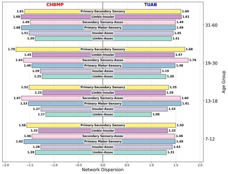
Fig. 7. TUAB and CHBMP datasets between-network dispersion across age groups.
4. Conclusion
In this paper, we propose an adaptive representation learning framework for electroencephalography-based brain age clustering (ARLC-Net). The model eliminates the need for predefined cluster numbers by reinforcing the learning mechanism to autonomously select optimal cluster numbers, effectively addressing the reliance of traditional clustering methods on predefined values. Extensive experimental results validate the superiority and effectiveness of ARLC-Net in EEG age clustering tasks. Building upon the clustering-derived age groupings, we investigated the spatial distribution of EEG patterns across neurodevelopmental stages. This analysis revealed novel connectivity phenomena that yield mechanistic insights into dynamic brain maturation processes.
Acknowledgments
This work was supported by the Major Science and Technology Program of Yunnan Province (Grant No.202102AA100021).
- [1] X. Di and B. B. Biswal, “Toward Task Connectomics: Examining Whole-Brain Task Modulated Connectivity in Different Task Domains,” Cerebral Cortex, Vol.29, Issue 4, pp. 1572-1583, 2019. https://doi.org/10.1093/cercor/bhy055
- [2] F. Zamani Esfahlani, J. Faskowitz, J. Slack, B. Mišić, and R. F. Betzel, “Local structure-function relationships in human brain networks across the lifespan,” Nature Communications, Vol.13, No.1, Article No.2053, 2022. https://doi.org/10.1038/s41467-022-29770-y
- [3] F. Di Gregorio and S. Battaglia, “Advances in EEG-based functional connectivity approaches to the study of the central nervous system in health and disease,” Advances in Clinical and Experimental Medicine, Vol.32, No.6, pp. 607-612, 2023. https://doi.org/https://dx.doi.org/10.17219/acem/166476
- [4] M. Wang, J. Hu, and H. A. Abbass, “BrainPrint: EEG biometric identification based on analyzing brain connectivity graphs,” Pattern Recognition, Vol.105, Article No.107381, 2020. https://doi.org/10.1016/j.patcog.2020.107381
- [5] S. Morales and M. E. Bowers, “Time-frequency analysis methods and their application in developmental EEG data,” Developmental Cognitive Neuroscience, Vol.54, Article No.101067, 2022. https://doi.org/10.1016/j.dcn.2022.101067
- [6] S. Coelli, M. Corda, and A. M. Bianchi, “The time-varying brain: A comprehensive review of dynamic functional connectivity analysis in EEG and MEG,” J. of Neural Engineering, Vol.22, No.5, 2025. https://doi.org/10.1088/1741-2552/ae1258
- [7] E. R. Paitel, C. B. D. Otteman, M. C. Polking, H. J. Licht, and K. A. Nielson, “Functional and effective EEG connectivity patterns in Alzheimer’s disease and mild cognitive impairment: A systematic review,” Frontiers in Aging Neuroscience, Vol.17, Article No.1496235, 2025. https://doi.org/10.3389/fnagi.2025.1496235
- [8] S. Marek, B. Tervo-Clemmens, N. Klein, W. Foran, A. S. Ghuman, and B. Luna, “Adolescent development of cortical oscillations: Power, phase, and support of cognitive maturation,” PLoS Biology, Vol.16, No.11, Article No.e2004188, 2018. https://doi.org/10.1371/journal.pbio.2004188
- [9] S.-B. Wong, Y. Tsao, W.-H. Tsai, T.-S. Wang, H.-C. Wu, and S.-S. Wang, “Author Correction: Application of bi-directional long-short-term memory network in cognitive age prediction based on EEG signals,” Scientific Reports, Vol.14, Article No.5433, 2024. https://doi.org/10.1038/s41598-024-53922-3
- [10] Y. Li, X. Zhang, J. Nie, G. Zhang, R. Fang, X. Xu, Z. Wu, D. Hu, L. Wang, H. Zhang, W. Lin, and G. Li, “Brain Connectivity Based Graph Convolutional Networks and Its Application to Infant Age Prediction,” IEEE Trans. on Medical Imaging, Vol.41, Issue 10, pp. 2764-2776, 2022. https://doi.org/10.1109/TMI.2022.3171778
- [11] J. Wang, J. Zhao, and T. Cheng, “SGAAE-AC: A Semi-Supervised Graph Attention Autoencoder for Electroencephalography (EEG) Age Clustering,” Applied Sciences, Vol.14, No.13, Article No.5392, 2024. https://doi.org/10.3390/app14135392
- [12] W. Song, M. Li, P. Zhang, Y. Wu, L. Jia, and L. An, “Unsupervised PolSAR Image Classification and Segmentation Using Dirichlet Process Mixture Model and Markov Random Fields with Similarity Measure,” IEEE J. of Selected Topics in Applied Earth Observations and Remote Sensing, Vol.10, Issue 8, pp. 3556-3568, 2017. https://doi.org/10.1109/JSTARS.2017.2684301
- [13] M. Kobayashi and K. Watanabe, “Generalized Dirichlet-Process-Means for Robust and Maximum Distortion Criteria,” 2018 Int. Symp. on Information Theory and Its Applications (ISITA), pp. 45-49, 2018. https://doi.org/10.23919/ISITA.2018.8664260
- [14] M. A. Asghar, M. J. Khan, M. Rizwan, R. M. Mehmood, and S.-H. Kim, “An Innovative Multi-Model Neural Network Approach for Feature Selection in Emotion Recognition Using Deep Feature Clustering,” Sensors, Vol.20, Issue 13, Article No.3765, 2020. https://doi.org/10.3390/s20133765
- [15] C. Niu, M. Wu, and L. Zhou, “Dual-Adaptive Fusion Multi-View Clustering Based on Graph Autoencoder,” 2024 Int. Joint Conf. on Neural Networks (IJCNN), 2024. https://doi.org/10.1109/IJCNN60899.2024.10650084
- [16] Q. Wang, F. Wang, F. Ren, Z. Li, and F. Nie, “An Effective Clustering Optimization Method for Unsupervised Linear Discriminant Analysis,” IEEE Trans. on Knowledge and Data Engineering, Vol.35, Issue 4, pp. 3444-3457, 2023. https://doi.org/10.1109/TKDE.2021.3124023
- [17] J. Tabbal, A. Ebadi, A. Mheich, A. Kabbara, B. Güntekin, G. Yener, V. Paban, U. Gschwandtner, P. Fuhr, M. Verin et al., “Characterizing the heterogeneity of neurodegenerative diseases through EEG normative modeling,” npj Parkinson’s Disease, Vol.11, Article No.117, 2025. https://doi.org/10.1038/s41531-025-00957-6
- [18] D. K. Hu, M. A. Pinto-Orellana, M. Rana, L. Do, D. J. Adams, S. A. Hussain, D. W. Shrey, and B. A. Lopour, “Discovering EEG biomarkers of Lennox-Gastaut syndrome through unsupervised time-frequency analysis,” Epilepsia, Vol.66, Issue 2, pp. 541-553, 2025. https://doi.org/10.1111/epi.18211
- [19] T. M. Rutkowski, T. Komendziński, and M. Otake-Matsuura, “Mild cognitive impairment prediction and cognitive score regression in the elderly using EEG topological data analysis and machine learning with awareness assessed in affective reminiscent paradigm,” Frontiers in Aging Neuroscience, Vol.15, Article No.1294139, 2024. https://doi.org/10.3389/fnagi.2023.1294139
- [20] L. E. Ismail and W. Karwowski, “A Graph Theory-Based Modeling of Functional Brain Connectivity Based on EEG: A Systematic Review in the Context of Neuroergonomics,” IEEE Access, Vol.8, pp. 155103-155135, 2020. https://doi.org/10.1109/ACCESS.2020.3018995
- [21] T. Balasuntharam, H. Davoudi, and M. Ebrahimi, “Preferential Proximal Policy Optimization,” 2023 Int. Conf. on Machine Learning and Applications (ICMLA), pp. 293-300, 2023. https://doi.org/10.1109/ICMLA58977.2023.00048
- [22] J. Yang, J. Cai, L. Zhong, Y. Pi, and S. Wang, “Deep Masked Graph Node Clustering,” IEEE Trans. on Computational Social Systems, Vol.11, Issue 6, pp. 7257-7270, 2024. https://doi.org/10.1109/TCSS.2024.3401218
- [23] N. Mrabah, M. Bouguessa, and R. Ksantini, “A contrastive variational graph auto-encoder for node clustering,” Pattern Recognition, Vol.149, Article No.110209, 2024. https://doi.org/10.1016/j.patcog.2023.110209
- [24] J. Bian, C. Dai, and G. Li, “Adaptive channel-weight dual-constrained semi-supervised EEG clustering,” Biomedical Signal Processing and Control, Vol.98, Article No.106720, 2024. https://doi.org/10.1016/j.bspc.2024.106720
- [25] Z. Peng, H. Liu, Y. Jia, and J. Hou, “EGRC-Net: Embedding-Induced Graph Refinement Clustering Network,” IEEE Trans. on Image Processing, Vol.32, pp. 6457-6468, 2023. https://doi.org/10.1109/TIP.2023.3333557
- [26] A. Tsitsulin, J. Palowitch, B. Perozzi, and E. Müller, “Graph Clustering with Graph Neural Networks,” J. of Machine Learning Research, Vol.24, No.127, pp. 1-21, 2023.
- [27] Y. Liu, X. Yang, S. Zhou, X. Liu, S. Wang, K. Liang, W. Tu, and L. Li, “Simple Contrastive Graph Clustering,” IEEE Trans. on Neural Networks and Learning Systems, Vol.35, Issue 10, pp. 13789-13800, 2024. https://doi.org/10.1109/TNNLS.2023.3271871
- [28] G. Li, D. Li, and C. Dai, “ssvEEGc: An efficient EEG clustering method using balance-constrained voting mechanism,” Biomedical Signal Processing and Control, Vol.81, Article No.104539, 2023. https://doi.org/10.1016/j.bspc.2022.104539
- [29] N. Mrabah, M. Bouguessa, M. F. Touati, and R. Ksantini, “Rethinking Graph Auto-Encoder Models for Attributed Graph Clustering,” IEEE Trans. on Knowledge and Data Engineering, Vol.35, Issue 9, pp. 9037-9053, 2023. https://doi.org/10.1109/TKDE.2022.3220948
- [30] Y. Liu, W. Tu, S. Zhou, X. Liu, L. Song, X. Yang, and E. Zhu, “Deep Graph Clustering via Dual Correlation Reduction,” Proc. of the AAAI Conf. on Artificial Intelligence, Vol.36, No.7, pp. 7603-7611, 2022. https://doi.org/10.1609/aaai.v36i7.20726
- [31] C. Dai, J. Wu, J. J. M. Monaghan, G. Li, H. Peng, S. I. Becker, and D. McAlpine, “Semi-Supervised EEG Clustering with Multiple Constraints,” IEEE Trans. on Knowledge and Data Engineering, Vol.35, Issue 8, pp. 8529-8544, 2023. https://doi.org/10.1109/TKDE.2022.3206330
- [32] Z. Peng, H. Liu, Y. Jia, and J. Hou, “Attention-driven Graph Clustering Network,” Proc. of the 29th ACM Int. Conf. on Multimedia (MM’21), pp. 935-943, 2021. https://doi.org/10.1145/3474085.3475276
- [33] C. Dai, J. Wu, D. Pi, L. Cui, B. Johnson, and S. I. Becker, “Electroencephalogram Signal Clustering with Convex Cooperative Games,” IEEE Trans. on Knowledge and Data Engineering, Vol.34, Issue 12, pp. 5755-5769, 2022. https://doi.org/10.1109/TKDE.2021.3060742
- [34] S. Pan, R. Hu, G. Long, J. Jiang, L. Yao, and C. Zhang, “Adversarially Regularized Graph Autoencoder for Graph Embedding,” arXiv preprint, arXiv:1802.04407, 2019. https://doi.org/10.48550/arXiv.1802.04407
- [35] I. Obeid and J. Picone, “The Temple University Hospital EEG Data Corpus,” Frontiers in Neuroscience, Vol.10, Article No.196, 2016. https://doi.org/10.3389/fnins.2016.00196
- [36] P. A. Valdes-Sosa, L. Galan-Garcia, J. Bosch-Bayard, M. L. Bringas-Vega, E. Aubert-Vazquez, I. Rodriguez-Gil, S. Das, C. Madjar, T. Virues-Alba, Z. Mohades et al., “The Cuban Human Brain Mapping Project, a young and middle age population-based EEG, MRI, and cognition dataset,” Scientific Data, Vol.8, Article No.45, 2021. https://doi.org/10.1038/s41597-021-00829-7
- [37] P. J. Rousseeuw, “Silhouettes: A graphical aid to the interpretation and validation of cluster analysis,” J. of Computational and Applied Mathematics, Vol.20, pp. 53-65, 1987. https://doi.org/10.1016/0377-0427(87)90125-7
- [38] T. Caliński and J. Harabasz, “A dendrite method for cluster analysis,” Communications in Statistics, Vol.3, Issue 1, pp. 1-27, 1974. https://doi.org/10.1080/03610927408827101
- [39] D. L. Davies and D. W. Bouldin, “A Cluster Separation Measure,” IEEE Trans. on Pattern Analysis and Machine Intelligence, Vol.PAMI-1, Issue 2, pp. 224-227, 1979. https://doi.org/10.1109/TPAMI.1979.4766909
- [40] A. Likas, N. Vlassis, and J. J. Verbeek, “The global -means clustering algorithm,” Pattern Recognition, Vol.36, Issue 2, pp. 451-461, 2003. https://doi.org/10.1016/S0031-3203(02)00060-2
- [41] S. V. Ülker, M. Çınaroğlu, E. Yılmazer, and S. Tarlacı, “Theta Cordance Decline in Frontal and Temporal Cortices: Longitudinal Evidence of Regional Cortical Aging,” J. of Clinical Medicine, Vol.14, Issue 23, Article No.8341, 2025. https://doi.org/10.3390/jcm14238341
- [42] Z. Kardos, B. Tóth, R. Boha, B. File, and M. Molnár, “Age-related changes of frontal-midline theta is predictive of efficient memory maintenance,” Neuroscience, Vol.273, pp. 152-162, 2014. https://doi.org/10.1016/j.neuroscience.2014.04.071
- [43] E. Huizeling, H. Wang, C. Holland, and K. Kessler, “Changes in theta and alpha oscillatory signatures of attentional control in older and middle age,” European J. of Neuroscience, Vol.54, Issue 1, pp. 4314-4337, 2021. https://doi.org/10.1111/ejn.15259
- [44] E.-M. Kurz, L. Bastian, M. Mölle, J. Born, and M. Friedrich, “Development of slow oscillation–spindle coupling from infancy to toddlerhood,” Sleep Advances, Vol.5, Issue 1, Article No.zpae084, 2024. https://doi.org/10.1093/sleepadvances/zpae084
- [45] A.-L. Satomaa, T. Mäkelä, O. Saarenpää-Heikkilä, A. Kylliäinen, E. Huupponen, and S.-L. Himanen, “Slow-wave activity and sigma activities are associated with psychomotor development at 8 months of age,” Sleep, Vol.43, Issue 9, Article No.zsaa061, 2020. https://doi.org/10.1093/sleep/zsaa061
This article is published under a Creative Commons Attribution-NoDerivatives 4.0 Internationa License.