
Research Paper:
Deep Learning for the Production of Official Statistics: Density Ratio Estimation Using Biased Transaction Data for Japanese Labor Statistics
Yuya Takada*,**
 , Yuri Murayama*
, and Kiyoshi Izumi*
, Yuri Murayama*
, and Kiyoshi Izumi*
*Department of Systems Innovation, School of Engineering, The University of Tokyo
7-3-1 Hongo, Bunkyo-ku, Tokyo 113-8656, Japan
**Re Data Science Co., Ltd.
Kashiwa-no-ha Open Innovation Lab, 178-4 Wakashiba, Kashiwa, Chiba 277-0871, Japan

National statistical offices are exploring alternative data sources for official statistics. Such data, including point-of-sale (POS) records and mobile phone GPS logs, are originally collected for operational rather than statistical purposes. In the era of big data, the private sector accumulates vast volumes of transaction data, and leveraging such data for official statistics has become an emerging priority. However, these efforts face significant challenges, primarily due to severe selection bias stemming from such data. Prior research has shown that, even if non-representative, transaction data can produce timely statistics via density ratio estimation methods from machine learning. As a proof of concept, that study demonstrated that preliminary estimates could be generated using biased data from a Japanese private employment agency, enabling the early release of a labor market indicator otherwise delayed by up to a year. Building on this, the present study incorporates deep learning into density ratio estimation to improve accuracy. While deep learning, when applied to density ratio estimation, is often considered prone to overfitting, this study demonstrates that it can improve estimation accuracy without overfitting. Moreover, although deep learning is typically regarded as requiring extensive hyperparameter tuning, we show that it can be implemented without a significant tuning burden, supporting its practical use in the production of official statistics.
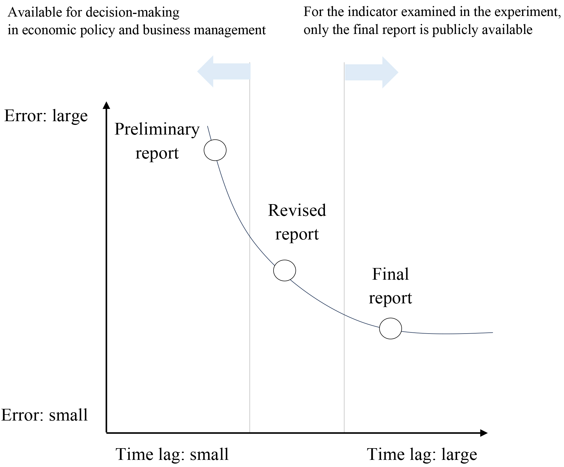
Errors and time lags in official statistics
1. Introduction
In recent years, national statistical institutes have increasingly adopted non-traditional data sources for the production of official statistics. These data sources are not originally intended for statistical purposes, as they are collected for objectives other than the generation of official statistics. For instance, point-of-sale (POS) data recorded in retail stores, real-time population data derived from mobile phone GPS logs, price information aggregated from hundreds of online retailers, satellite imagery, and internet search trends—such as those published in Google Trends—can all be utilized to construct official statistics.
These emerging data sources have the potential to significantly enhance the utility of official statistics. If economic conditions can be captured more comprehensively and in a timelier manner through such sources, it is reasonable to expect improvements in the quality of decision-making, including economic policy formulation.
In the era of big data, private companies accumulate vast volumes of transaction data. It is therefore imperative to explore avenues for incorporating these data into the production of official statistics. However, the pace of progress in utilizing such data has been slower than anticipated. This is primarily because most of these data cannot be directly employed for statistical purposes. As they are not collected through survey methodologies grounded in sample design, they exhibit substantial selection bias when considered as potential sources for official statistics. In other words, if this pronounced selection bias can be appropriately corrected, a considerable volume of valuable transaction data could be effectively leveraged as a basis for official statistics, thereby expanding their scope and enhancing the quality of diverse policy and business decisions.
Previous studies 1,2 have proposed frameworks for producing official statistics using new data sources subject to selection bias—particularly transaction data collected for operational rather than statistical purposes and not derived from survey-based methodologies. Specifically, prior work introduced a framework for generating preliminary reports based on partial datasets that, while biased, offer high timeliness. This approach is especially relevant for indicators where comprehensive nationwide data are eventually available for official statistics, but long publication lags reduce their usefulness for timely policy responses. In this context, the previous study emphasizes timeliness as a key advantage of new data sources. Surveys designed for the production of official statistics are inherently time-consuming due to the need to collect responses from firms or households. In contrast, the proposed framework can access new data sources with minimal lag—yesterday’s data become available the next day. If this framework enables the production of official statistics that reflect current economic conditions more promptly, it is reasonable to anticipate improvements in the quality of decision-making, including economic policy planning.
The problem of inferring population-level characteristics from biased data samples is a well-known challenge in machine learning, and extensive research has addressed this issue. In this light, integrating machine learning techniques into the production of official statistics holds the potential to fundamentally resolve longstanding challenges in the field. The aforementioned study focuses on methodologies rooted in machine learning—specifically, density ratio estimation and the concept of covariate shift.
In the present study, we demonstrate that the application of deep learning to the approach proposed in 1,2 can further enhance estimation accuracy. In doing so, we adopt the methodology introduced in 3, which formulates a framework for Bregman divergence minimization. This framework offers a unified view of various density ratio estimation methods and investigates its applicability to highly flexible models such as deep neural networks. According to 4, recent advances in machine learning have highlighted the superior performance of deep neural networks in diverse domains including computer vision 5 and natural language processing 6, thus motivating their application to density ratio estimation. However, employing Bregman divergence minimization with highly flexible models introduces the risk of overfitting, particularly in the form of train loss hacking, which arises from properties of empirical Bregman divergence estimators. To mitigate this issue, 4 proposes a non-negative correction to the empirical estimates, thereby stabilizing the training process and reducing overfitting.
Following the methodology of 1,2, we experimentally confirm that prompt preliminary statistics can be generated using biased data from a Japanese private employment agency.
For policymakers, corporate decision-makers, and recruitment professionals, timely insights into labor market trends are essential. To support this need, various official labor statistics are available in many countries, offering metrics such as unemployment rates, labor force counts, and average wages—typically published with a lag of two to three months. However, some indicators remain difficult to capture in a timely manner, with publication delays exceeding one year. One such indicator is the wage changes upon job change, capturing the pressure exerted on wages by supply–demand conditions in the external labor market. The timely release of this indicator would greatly benefit those involved in public policy, corporate management, and recruitment.
Among the various potential measures of the wage changes upon job change, this study adopts the proportion of job switchers who experience a wage increase, specifically those whose post-transition wages rise by more than 10%. The indicator is calculated as the ratio of individuals with a wage increase exceeding 10% to the total number of job switchers within a given period. The “more than 10%” threshold signifies a significant increase, and thus the indicator reflects the proportion of individuals whose wages markedly improved following a career change. In official Japanese labor statistics, this indicator is released with a time lag ranging from 6 to 13 months. The central challenge addressed in this study is the elimination of this extended delay.
Career transitions in the external labor market occur through multiple channels, including job advertisements, public and private employment agencies, and personal referrals. In this study, we focus on transaction data maintained by private employment agencies, as these organizations possess such data in formats suitable for real-time analysis. Private agencies typically conduct interviews with job seekers, enabling accurate documentation of pre-transition wages. Moreover, as part of the job change process, these agencies calculate and present to job seekers the annual wages they would earn in the new position. Consequently, they inherently possess both pre- and post-transition wage data. In contrast, job transitions occurring via advertisements or referrals generally lack mechanisms for recording wage data. While public employment agencies, in principle, could collect such information for statistical purposes, this system has not been fully implemented in Japan.
We obtained transaction data from the largest private employment agency in Japan. Additionally, we were granted access to anonymized sample data from official government statistics—unavailable to the general public—for benchmarking purposes. Both datasets consist of raw micro-level data rather than pre-tabulated statistics. Most of the processing in this study is conducted at the individual data level, not on aggregated statistical tables. It is important to emphasize that individuals cannot be identified and that strict data protection protocols have been observed throughout this study.
Although transaction data from private employment agencies are available in real time, their population coverage is limited—less than 5% even for the largest agency used in this study. Moreover, when used as a sample to infer trends at the national level, these data exhibit considerable bias. For example, in the second half of 2018, the average age of full-time job changers in the official statistics was approximately 40 years, whereas it was around 31 years in the transaction data. Similarly, the share of individuals with a university degree or higher was about 35% in the official data, compared to 79% in the transaction data. These discrepancies highlight the substantial sampling bias inherent in the transaction data.
This bias arises because the sample is limited to individuals who changed jobs through private employment agencies—namely, those firms who are willing to hire even when paying agency fees. In contrast, although official statistics are subject to significant publication delays, they capture a comprehensive view of national labor market dynamics. Therefore, if the relationship between private agency transaction data and official statistics can be learned and used to correct the bias in the former, the challenge can be effectively addressed.
The previous studies 1,2 demonstrated the feasibility of correcting selection bias through density ratio estimation combined with covariate shift correction. Building upon that foundation, the present study introduces deep learning to further improve estimation accuracy. The main contributions of this study are as follows.
Although deep learning is generally considered prone to overfitting when applied to density ratio estimation, this study improves estimation accuracy without inducing overfitting.
It further shows that deep learning can be applied effectively without extensive hyperparameter tuning, demonstrating its practical applicability to the production of official statistics.
It should be noted that the proposed framework is not limited to labor statistics, but can also be applied to other statistical domains that exhibit similar structural biases.
2. Related Work
As noted in the previous section, national statistical institutes have recently begun adopting non-traditional data sources for the production of official statistics. These new data sources are not inherently designed for statistical purposes. The transaction data from private employment agencies used in this study fall into this category. Other examples have also been documented in the literature, where a variety of alternative data—such as satellite imagery, GPS-based population data from mobile phones, POS records from retail outlets, online price information, and internet search trends like Google Trends—have been employed in the production of official statistics.
The International Telecommunication Union (ITU), a United Nations agency specializing in information and communication technology, has been at the forefront of utilizing GPS-based real-time population data from mobile phones. As the secretariat of the Mobile Data Task Team within the United Nations Statistics Division, the ITU has promoted the global adoption of such data sources 7. Between 2016 and 2018, countries including Colombia, Georgia, Kenya, the Philippines, Sweden, and the UAE collected and processed data from telecom providers to complement household surveys and official registries, yielding 16 distinct indicators. During 2020–2021, Brazil and Indonesia conducted studies leveraging telecom data to assess two Sustainable Development Goal indicators: mobile network coverage and internet access. To support broader adoption, the ITU published the Handbook on the Use of Mobile Phone Data for Official Statistics 8. In Estonia, due to budget constraints, traditional travel surveys were replaced with mobile SIM card data to monitor travel expenditures 9.
Since the early 2000s, the use of POS data has expanded significantly across numerous countries. Notably, Switzerland, Norway, and the Netherlands have undertaken dedicated efforts to incorporate POS data as a way to overcome limitations of conventional data sources. Beginning with the study cited in 10, new price indices based on POS data have been developed and validated in subsequent research 11,12. In Japan, a private company provides price indices constructed from POS data in accordance with the methodology described in 13. These indices are utilized by the Bank of Japan in various official reports. Additionally, price indices have been created using price data collected from a wide range of online retailers. The Billion Prices Project, launched in 2008 by Professors Alberto Cavallo and Roberto Rigobon at MIT Sloan and Harvard Business School, introduced novel price indices based on online retail data 14,15, as well as a new methodology for constructing purchasing power parities (PPPs) 16.
The Organisation for Economic Co-operation and Development (OECD) has employed internet search data from Google Trends in its statistical initiatives. These data contribute to the publication of the OECD Weekly Tracker of Economic Activity, which estimates weekly GDP for 46 countries, including OECD and G20 members 17. Google Trends data have also been used in estimating unemployment rates 18, serving as an auxiliary time series for the nowcasting of monthly unemployment statistics alongside the official labor force survey.
The studies most closely related to the present work are 1 and 2, also discussed in Section 1. Among them, 2 shares not only the methodological framework but also the experimental setting with the present study, and thus is used as a benchmark reference for comparison with this research. Both studies, however, are based on the same overall methodological framework. Those studies propose a framework for producing timely indicators of wage changes among job changers in Japan by utilizing transaction data from a private recruitment agency. The data sample is limited to individuals who changed jobs via private recruitment services, excluding those who transitioned through job advertisements, personal referrals, or public employment services. Compared to the datasets employed in the other cases described above, this results in a stronger degree of selection bias. To address this issue, 1,2 apply methodologies developed in the field of machine learning, particularly density ratio estimation and the concept of covariate shift.
3. Task Setting
In this section, we describe the task structure, evaluation method, and the positioning of the present experiment within the typology of selection bias, following 2. To maintain generality in the discussion, we do not elaborate on specific experimental settings or data details here; those will be provided in Section 5, following the methodological exposition in Section 4.
Fig. 1. Errors and time lags in official statistics. This figure is adapted from 2.
3.1. Structure of the Task
Official statistics are typically published in multiple stages, such as preliminary, revised, and final releases. Naturally, earlier releases tend to be less accurate, whereas later ones offer greater precision. In most cases, only the preliminary indicators are available in time to support economic policy and business decision-making. This structure is illustrated in Fig. 1, where the term error is used schematically to represent the discrepancy between the true statistical value—which is fundamentally unobservable—and the value obtained through surveys.
However, many important indicators in official statistics do not include preliminary releases suitable for timely decision-making. This is often due to difficulties such as the high cost of surveys or the burden placed on businesses, which complicate rapid data collection and publication. The present study focuses on such indicators. As shown in Fig. 1, for the indicator used in our experiment, only the final report is publicly available. In this study, we demonstrate that it is possible to construct a preliminary report even for such indicators.
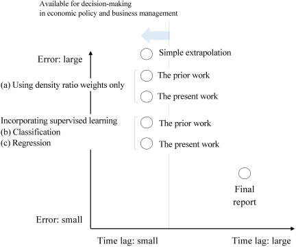
Fig. 2. Structure of the experimental design. This figure is adapted from 2.
In Fig. 1, the term error schematically represents the discrepancy between the true, unobservable statistical value and the survey-based observed value. However, because the true values are unobservable in this study, we treat the final released statistics as ground truth and evaluate the accuracy of our preliminary estimates by measuring the difference between the estimated and final values. To assess estimation performance, we employ the mean absolute error (MAE). Specifically, the MAE is calculated by comparing our estimated proportion of individuals who experienced wage increases after changing careers with the corresponding values published by the government.
As mentioned earlier, this study aims to improve estimation accuracy by incorporating deep learning into the framework proposed in 2. Accordingly, we evaluate whether the MAE is further reduced under the same experimental settings used in the previous study.
3.2. Evaluation
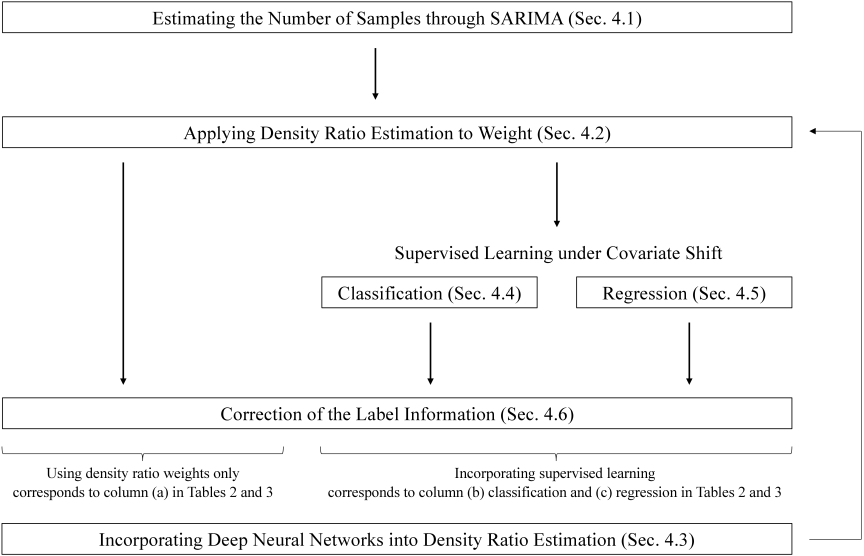
Fig. 3. Architecture of the estimation. This figure was created by the author with reference to 2.
We focus on MAE because it provides an interpretable measure of average deviation in percentage points and is robust to extreme observations, which is particularly relevant in macroeconomic time-series settings with a limited number of evaluation periods. For reference, we also confirmed that the two key findings reported in Section 6 are qualitatively similar when alternative evaluation metrics such as MSE and RMSE are used (results omitted for brevity).
Both the previous and present studies consider the following estimation strategies: (a) using the estimated density ratio solely as a weight, (b) incorporating an additional supervised learning step (classification), and (c) incorporating an additional supervised learning step (regression). In Fig. 3 in Section 4, the leftmost panel corresponds to (a), the center panel corresponds to (b), and the right panel corresponds to (c). The comparative framework underlying these strategies is illustrated in Fig. 2.
As in the prior work, we also report a simple extrapolation-based prediction as a baseline, which is defined by the following equation. This baseline reflects a setting in which no correction for selection bias is applied:
In relation to the notation used in Section 4, \(o_{T}\) corresponds to the number of components equal to 1 in the vector \(Y_{g,T}\), divided by the number of dimensions. Likewise, \(s_{T}\) corresponds to the number of components equal to 1 in the vector \(Y_{p,T}\) (under a classification label setting), divided by the number of dimensions.
3.3. Types of Selection Bias and Position of this Study
The task addressed in this study is closely related to the covariate shift framework. Covariate shift refers to a situation in which the distributions of input variables differ between training and test datasets, while the conditional distribution of output given input remains unchanged. This scenario is frequently encountered in machine learning 19.
Let \(\mathcal{D} \subset \mathbb{R}^{d}\) be the covariate space, where \(d\) is a positive integer. Let \(x \in \mathcal{D}\) and \(y \in \mathcal{D}' \subset \mathbb{R}\) denote a covariate and its corresponding label, respectively. Let \(p_S\) and \(p_T\) represent the training and test distributions. Under these definitions, the covariate shift setting is defined as:
Under covariate shift, standard learning methods such as maximum likelihood estimation yield biased results. However, this bias can be asymptotically corrected by weighting the loss function according to the density ratio 20.
Covariate shift is considered a specific subclass of selection bias. Since 21, sample selection bias has typically been categorized into three missing data mechanisms: MCAR, MAR, and NMAR.
-
MCAR (Missing Completely at Random): The probability of missingness is unrelated to the missing values themselves or to any observed data.
-
MAR (Missing at Random): The probability of missingness depends only on the observed data, not on the unobserved values.
-
NMAR (Not Missing at Random): The probability of missingness depends on the missing values themselves, making the mechanism non-random.
According to 22, the covariate shift assumption is equivalent to the MAR condition. However, as noted in 23, MAR and NMAR are not fundamentally distinct but rather exist on a continuum. In this study, the situation we address is more appropriately considered to fall closer to the NMAR category.
In NMAR cases, 24 states that the response probability cannot be inferred solely from the observed variables, and thus additional modeling assumptions are typically required. The correction method described in Section 4.6 reflects such an additional assumption.
4. Methodology
This section presents the methodological framework of our study. Fig. 3 illustrates the overall architecture of the proposed estimation procedure. This study proposes the application of deep learning to the step corresponding to the second layer from the top in Fig. 3. Section 4.2 outlines the methodological framework common to the prior studies 1,2. Subsequently, Section 4.3 provides a detailed description of the newly introduced deep learning approach adopted in this study. Accordingly, Section 4.3 represents the primary methodological contribution and the key difference from the existing studies. Note that the prior studies 1,2 provide more detailed explanations with figures for Sections 4.1, 4.2, 4.4, 4.5, and 4.6; therefore, we only provide a brief overview here.
4.1. Estimating the Number of Samples and Their Attributes Through SARIMA
We first estimate the number of samples for the target half-year across different job transition channels and obtain attribute information for each sample. In this phase, we do not acquire label information for individual samples in the target half-year. The number of samples is estimated using SARIMA, based on the time series of sample counts by transition channel (e.g., public employment offices, private agencies, job advertisements, personal connections). Model parameters are selected using the Akaike information criterion (AIC). Attribute information for each sample is generated by duplicate random sampling from the most recent available real data, typically from the same period one year earlier.
Let \(Y_{g,t}\) denote a vector of label information from government survey samples at time \(t\), where each component represents whether an individual received a wage increase of over 10% after changing jobs. The number of vector elements corresponds to the sample size. Let \(X_{g,t}\) be the matrix of associated attribute information (e.g., age, gender, education), as detailed in Section 5.2. Similarly, \(Y_{p,t}\) and \(X_{p,t}\) denote the label vector and attribute matrix, respectively, for private employment agency samples.
In this step, we estimate \(X_{g,T-1}\) and \(X_{g,T}\) using SARIMA applied to sample counts from \(T-k\) to \(T-2\), and duplicate sampling from \(X_{g,T-2}\). We do not estimate or use \(Y_{g,T-1}\), \(Y_{g,T}\), \(Y_{p}\), or \(X_{p}\) in this phase.
4.2. Applying Density Ratio Estimation to Weight Private Agency Samples
In this step, we compute the sample weights \(w_{T}\) using \(Y_{p,T}\), \(X_{p,T}\), and \(X_{g,T}\) obtained in the previous step, employing density ratio estimation. The density ratio estimation problem is formalized as follows 19. Let \(\mathcal{D} \subset \mathbb{R}^d\) be the data domain, where \(d\) is a positive integer. Suppose we have i.i.d. samples \(\{x_i\}_{i=1}^n\) from a distribution \(p_S(x)\), and i.i.d. samples \(\{x'_j\}_{j=1}^{n'}\) from a different distribution \(p_T(x)\), both defined over \(\mathcal{D}\). The goal is to estimate the density ratio \(w(x) = p_T(x) / p_S(x)\).
4.3. Incorporating Deep Neural Networks into Density Ratio Estimation
In the previous studies 1,2, uLSIF 25 was adopted for density ratio estimation, where the model employed was linear-in-parameter, with nonlinear structures captured through kernel functions and regularization introduced to prevent overfitting. In contrast, the model in this study is a deep neural network, and we investigate the potential for improving the accuracy of density ratio estimation. Section 4.3.1 presents the concept of density ratio matching based on Bregman divergence, showing that uLSIF is a special case within this framework. Section 4.3.3 discusses the overfitting issue known as train loss hacking, which arises when performing density ratio matching with deep neural networks under the Bregman divergence framework. Finally, Section 4.3.4 introduces the non-negative Bregman divergence estimator, a recently proposed method for improving the robustness of empirical Bregman divergence estimators against train loss hacking.
4.3.1. Density Ratio Matching by Bregman Divergence Minimization
Following 3, this section introduces the concept of density ratio matching using Bregman divergence, and shows that the uLSIF method presented in the previous section is a special case within this broader framework. This formulation generalizes the least-squares approach and also encompasses other methods examined in 1,2, such as moment matching 26,27, probabilistic classification 28,29,30, density matching 31,32,33,34,35, and density ratio fitting 25.
The objective is to estimate the density ratio:
The core idea of density ratio matching is to directly fit a density ratio model \(\hat{w}(x)\) to the true density ratio function \(w(x)\) under a specified divergence. While this may appear similar to regression, density ratio matching differs fundamentally in that samples of the true density ratio are not available. In this work, we use the Bregman divergence to quantify the discrepancy between \(w(x)\) and \(\hat{w}(x)\).
The Bregman divergence is a generalization of Euclidean distance. Let \(f\) be a differentiable, strictly convex function. Then the Bregman divergence from \(u^*\) to \(u\) is defined as:
The term \(f(u) + \partial f(u)(u^* - u)\) corresponds to the first-order Taylor expansion of \(f\) at \(u\), evaluated at \(u^*\). Thus, the Bregman divergence measures the difference between the true value of \(f(u^*)\) and its first-order linear approximation from \(u\). See Fig. 4 for illustration.
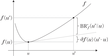
Fig. 4. Bregman divergence \(\text{BR}'_f(u^*\|u)\). This figure was created by the author with reference to 3.
The discrepancy between the true density ratio function \(w\) and the model \(\hat{w}\) is measured using the Bregman divergence, defined as
A key motivation for adopting this formulation is that the Bregman divergence enables a direct empirical approximation for any choice of \(f\). Specifically, we isolate the relevant component of \(\mathrm{BR}_f(\hat{w})\) as follows:
An empirical approximation \(\widehat{\mathrm{BR}}_f(\hat{w})\) of \(\mathrm{BR}_f(\hat{w})\) is then given by
This leads directly to the following optimization criterion:
4.3.2. uLSIF Within the Framework of Density Ratio Matching
We now demonstrate that LSIF/uLSIF, as used in 1,2, constitutes a special case of density ratio matching 3. Specifically, there exists a Bregman divergence for which the density ratio matching objective reduces to that of LSIF/uLSIF.
When
Equation 3 is reduced to the squared (SQ) distance:
Following Eqs. 5 and 6, we denote the squared loss without the irrelevant constant term by \(\text{SQ}(\hat{w})\), and its empirical approximation by \(\widehat{\text{SQ}}(\hat{w})\), respectively:
4.3.3. Train Loss Hacking Problem
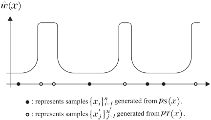
Fig. 5. The structure of the train loss hacking problem. This figure was created by the author with reference to 4.
We now discuss the overfitting problem known as train loss hacking, which arises when performing density ratio matching with deep neural networks under the Bregman divergence framework. Given the success of deep neural networks in fields such as computer vision 5 and natural language processing 6, their application to density ratio estimation represents a natural extension. However, naive application within the Bregman divergence framework can lead to substantial overfitting. For instance, 4 demonstrates that LSIF implemented with neural networks exhibits severe overfitting. One potential cause of this issue has been hypothesized to be train loss hacking—a phenomenon also discussed in a related context by 36 in the setting of positive-unlabeled (PU) learning.
The density ratio estimation problem has already been formulated in Section 4.3.1. The objective in this setting is to estimate the density ratio defined in Eq. 1, based on samples drawn from the source and target distributions \(p_{S}(x)\) and \(p_{T}(x)\).
Train loss hacking refers to a phenomenon in which \(\hat{w}(x)\) takes on excessively large values for \(\{ x'_j \}_{j=1}^{n'}~\mathrm{i.i.d.}~\sim p_{T}(x)\).
The structure of the train loss hacking problem is illustrated in Fig. 5.
This issue arises when a model is trained to minimize an objective function that involves multiple distinct sample sets. Specifically, in the case of density ratio matching under the Bregman divergence framework, the objective function defined in Eq. 6 consists of two empirical averages. Among these, the second term
Since \(f\) is a convex function, its derivative \(\partial f\) is monotonically increasing; thus, the second term decreases as \(\hat{w}(x'_j)\) increases. Consequently, when no lower bound exists for this term, it frequently diverges to negative infinity in numerical computations. Even if a bounded model is used for \(\hat{w}\), numerical instability often leads to divergence. Moreover, even when a lower bound is imposed, \(\hat{w}(x'_j)\) still tends to assume the maximum possible value within its output range at the points \(\{ x'_j \}_{j=1}^{n'}\). Simply capping the model’s output, for example, by applying \(\max\{\cdot, B\}\) with some constant \(B > 0\), does not resolve the issue, as the model still converges to its largest possible value.
This is a significant issue because merely increasing the output at \(\{ x'_j\}_{j=1}^{n'}\) does not constitute a valid training criterion for density ratio estimation, and it results in an unreasonable density ratio estimator. The problem becomes particularly severe in highly flexible models. If the hypothesis class is severely restricted, a trade-off may be introduced by the remaining term of Eq. 6:
However, in the case of highly flexible models, such as deep neural networks, the model can easily fit \(\{ x'_j \}_{j=1}^{n'}\) and \(\{ x_i \}_{i=1}^{n}\) separately.
4.3.4. Deep Learning for Density Ratio Estimation Using Non-Negative Risk Estimator
Naive application within the Bregman divergence framework leads to a significant overfitting issue, known as train loss hacking, as discussed in Section 4.3.3. This section introduces the non-negative Bregman divergence estimator 4, a method proposed to enhance the robustness of the empirical Bregman divergence estimator against train loss hacking.
To address this problem, 4 proposed a non-negative Bregman divergence estimator that modifies the empirical objective defined in Eq. 6 to improve robustness. According to 4, the method is inspired by 36, which introduces a non-negative correction to the empirical risk in PU learning, based on the observation that a portion of the population risk is inherently non-negative. However, in the context of density ratio estimation, it is not straightforward to apply this idea, since it is unclear which part of the population risk, as defined in Eq. 5, is non-negative. To overcome this, an upper bound \(\overline{W}\) is assumed for the density ratio \(w\), allowing the identification of a non-negative component of the population risk, as expressed in Eq. 3. A non-negative correction is then applied to the empirical Bregman divergence estimator based on this decomposition. This strategy also generalizes the concept of non-negative PU learning 36. To ensure that this method effectively mitigates train loss hacking, the following assumption must be satisfied:
Assumption 1
The density ratio \(w\) is bounded from above, i.e.,
Then, we specify a constant \(C\) such that \(0 < C < {1}/{\overline{W}}\). Based on this constant, we impose the following assumption.
Assumption 2
\(\tilde{f}\) defined by
Then, the Bregman divergence minimization objective given in Eq. 5 can be reformulated as
The first two terms in Eq. 12 are non-negative, as both \(\ell_{1}\) and \(p_{S} - C p_{T}\) are non-negative under Assumption 1 and the condition \(0 < C < {1}/{\overline{W}}\).
Motivated by this observation, the following modified empirical risk is proposed.
4.4. Supervised Learning Under Covariate Shift: Classification
We now perform supervised classification using the weighted private employment agency samples from Section 4.2. We aim to estimate a function \(F\) such that \(Y_{p,T} = F(X_{p,T})\), using the weights \(w_T\). Using the estimated function \(F\), we compute \(F(X_{g,T})\) and use the resulting classifier score in the subsequent step.
Three classifiers were tested in prior studies: logistic regression with an elastic net penalty, random forest, and gradient-boosted decision trees. Due to minimal differences in accuracy, we adopt only logistic regression with elastic net regularization in this study. All attributes listed in Section 5.2 are used as explanatory variables in \(X_{p,t}\).
Standard learning algorithms, such as maximum likelihood estimation, become biased under covariate shift, as described in Section 3.3. This bias can be asymptotically corrected using density ratio weighting 20.
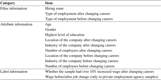
Table 1. List of variables used.
4.5. Supervised Learning Under Covariate Shift: Regression
In contrast to the binary labels in the government survey data, the private employment agency samples include continuous wage change ratios. To utilize this information, we perform regression analysis. Here, the label is defined as the ratio of post-transition to pre-transition wages (e.g., a 10% increase results in a label value of 1.1).
As in Section 4.4, three regression models were previously tested: linear regression with elastic net regularization, random forest, and gradient-boosted decision trees. Again, due to similar performance, we employ only the linear model. Attributes from Section 5.2 serve as inputs \(X_{p,T}\).
Before regression, \(Y_{p,t}\) is transformed using the Box-Cox transformation. After estimating \(F\), using \(Y_{p,t}\), \(X_{p,t}\), and the density ratio-based weight \(w_{t}\), we compute a classifier score as the probability that \(F(X_{g,T})\) exceeds the Box-Cox transformed threshold of 1.1, assuming normally distributed residuals. For example, if \(F(X_{g,T})\) equals the transformed 1.1 value, the resulting score is 0.5. This transformed score is then used in the subsequent step.
4.6. Correction of the Label Information
Using the outputs from Sections 4.2, 4.4, or 4.5, we obtain bias-corrected label information for the target half-year. This information can be directly used to compute the proportion of individuals who experienced wage increases. However, instead of using these estimates as is, we apply a correction method based on the assumptions discussed below.
As noted in Section 3, in this study, we consider the observed data mechanism closer to NMAR. In this study, the covariates listed in Table 1 are observable and provide rich information on individuals and firms. However, these covariates, while powerful, have inherent limitations. For example, the highest level of education helps distinguish between high school and college graduates, but it does not capture the quality of the institution, nor the difficulty of admission or graduation. Similarly, firm-level information such as location, firm size, and industry is available, but it does not indicate whether the firm attracts high-ability workers or offers superior working conditions. As a result, samples from the private employment agency may still suffer from selection bias driven by unobserved characteristics relative to the national population. This is the reason why the situation considered in this study is closer to the NMAR setting than the standard MAR assumption. According to 24, NMAR implies that response probabilities cannot be identified from observed data alone and require additional assumptions. In what follows, we outline such an assumption.
Under the covariate shift setting, the conditional distribution remains invariant, as described in Section 3.3.
However, as discussed above, in practice, the available attribute information is often insufficient to uphold this assumption. We thus adopt a relaxed assumption:
We multiply \(\beta\) by the values obtained in Sections 4.2, 4.4, or 4.5. In the case of Section 4.2, the values are weighted \(0/1\) labels, so we simply multiply by \(\beta\) and aggregate the counts. When multiplying by the classifier scores from Section 4.4 or the transformed scores from Section 4.5, the mean of these corrected scores is used to estimate the proportion of individuals with increased wages. While binary classification using a cutoff threshold was also considered, it was avoided due to the difficulty of determining an appropriate threshold.
5. Experiment
While Section 3 maintained a general perspective by providing an abstract overview of the task setting, this section presents the specific details of the experimental design that were not previously discussed. In particular, we describe the time lag structure of the official statistics used, the characteristics of the datasets, and the full details of the experimental procedure.
5.1. Time Lag Structure
The official statistics used in this experiment are based on a semiannual statistical survey and are subject to a publication delay of approximately six to thirteen months. Data collected from January to June are released at the end of December, whereas data from July to December are made public in late August of the following year. This substantial time lag prevents policymakers and human resource managers from using the data for timely decision-making.
To address this issue, we utilized transaction data from Recruit Agent, Japan’s largest private employment agency under the Recruit Holdings Co., Ltd. umbrella. This dataset is available with virtually no delay, enabling access to previous-day data on the following day. Accordingly, our objective is to enable the release of January–June period indicators in early July, and July–December indicators in early January, thereby reducing the time lag from several months to just a few days.
This study employs both job-changer samples obtained from government surveys and transaction data samples from private employment agencies. Government survey samples are available internally within the government immediately after collection but are made available to external parties only upon publication. We consider a realistic setting in which estimation is performed by an external organization. Letting \(T\) denote a six-month period, we assume that when private agency data from period \(T\) become available, government survey data are only available up to period \(T-2\).
5.2. Data Characteristics
In this study, we utilize two data sources: samples from a government survey and private employment agency samples.
We begin by describing the government survey samples used in this study. These samples were collected by the Ministry of Health, Labour and Welfare of Japan through a sample survey called the Survey on Employment Trends. While only aggregated statistical information is publicly available and the raw samples and weight data are not published, we obtained access to them through an official request.
Although the survey is conducted at the establishment level, it includes information on individual employees who joined the company. For this study, we utilized individual-level sample data along with their associated weights. In Section 4, \(Y_{g,t}\) and \(X_{g,t}\) represent the label vector and attribute matrix, respectively, for the government survey samples. The samples were replicated according to the proportions indicated by the weight information.
The survey is conducted semiannually. We used data from the first half of 2004 through the first half of 2018. In the first half of 2018, the number of new employee samples was 37,841. Based on the sample and weight information for that period, the estimated number of job changers published in the Survey on Employment Trends is approximately 2,671,100. Of these, around 1,651,400 were full-time employees and 1,019,800 were part-time workers. The list of available data fields is summarized in Table 1. Since our analysis focuses on full-time employees, part-time worker samples were excluded.
Second, we describe the private employment agency samples. These samples are derived from transaction data provided by the Recruit Agent service, operated by the private employment agency under Recruit Holdings Co., Ltd. The agency currently registers over 1,200,000 new job seekers annually and maintains more than 500,000 job offers. At present, approximately 50,000 individuals change jobs through this agency each year. The transaction data include job seekers’ attribute information, detailed job offer information, and records of the job search process, such as applications and interviews.
We preprocessed the transaction data to align with the data items used in the government survey described above. In addition, we obtained supplementary items that serve as label information. While the government survey data provide only categorical information indicating whether a respondent experienced over \(10\%\) wage growth after changing jobs, the transaction data include both pre- and post-transition wages as continuous values. This continuous label information was utilized for regression analysis, as explained in Section 4.5.
Although the transaction data are available in real time, the coverage rate is quite low—less than \(5\%\) even in the case of the largest agency examined in this study. Moreover, when the data are used as a sample to infer national-level trends, they exhibit significant bias. As an illustrative example, in the second half of 2018, the average age of full-time employees who changed jobs, according to the government survey, was approximately 40 years. In contrast, the corresponding figure in the transaction data was around 31 years. Similarly, the proportion of individuals holding a university degree or higher was about \(35\%\) in the official statistics, compared to approximately \(79\%\) in the transaction data. These differences reflect a substantial discrepancy between the two datasets.
5.3. Details of Experimental Design
To evaluate the performance of our estimation, we employed the MAE, as described in Section 3.2. The dataset used spans from the first half of 2004 to the second half of 2018, and the validation period ranges from the second half of 2013 to the second half of 2018.
For each target half-year within the validation period, we utilized government survey samples up to one year prior to the target half-year and private employment agency samples from the target half-year.
For example, as outlined in Section 4.1, we used government survey samples from the first half of 2004 to the second half of 2013 to estimate the second half of 2014 using SARIMA. Subsequently, as discussed in Section 4.2, we used private employment agency samples from the second half of 2014 to perform density ratio estimation via uLSIF.
In Section 4.6, the label information was corrected using a constant value \(\beta\), which was calculated as the ratio of two quantities: the numerator being the actual proportion of individuals with increased wages after changing careers, and the denominator being the corresponding estimated value without this correction.
We considered two approaches for computing \(\beta\). \(\beta\) is calculated using the ratio between the actual proportion of samples where \(Y=1\) in each period and its estimated value when label information is not corrected. In the first approach, \(\beta\) was calculated as the average of the ratios, which are the estimation results from the first half of 2013 to the most recent half-year preceding the target period. This setting ensures that only information available at the time of estimation is used. In the second approach, \(\beta\) was calculated as the average of the ratios, which are all the estimation results from the first half of 2013 to the second half of 2018. This setting assumes access to future data that would not have been available at the time of estimation and is therefore infeasible in practice. Under the first approach, relatively more information is available for later periods in the test window, whereas information is more limited for earlier periods. In contrast, the second approach uses richer and more uniform information across all periods. Thus, the second approach can be interpreted as a reference case that provides an upper bound on achievable performance under the assumption of time-invariant the ratio. However, this interpretation is valid only if the ratio is approximately time-invariant. If the ratio is unstable over time, the results under the second approach could be worse than those under the first approach.
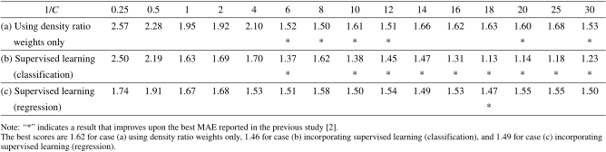
Table 2. MAE: The case of calculating \(\beta\) from the results before the target period.
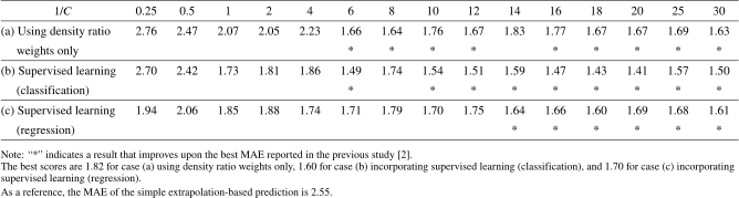
Table 3. MAE: The case of calculating \(\beta\) from all results.
6. Results
As mentioned in Section 3.2, this study aims to demonstrate improved estimation accuracy by applying deep learning to the approach proposed in the prior work 2. Accordingly, we show that the MAE is further reduced under the same experimental settings as used in the prior study.
Both the prior study and the present work consider two estimation strategies: one that uses the estimated density ratio solely as a weight, and another that incorporates an additional supervised learning step. In Fig. 3 in Section 4, the leftmost case corresponds to the former approach, while the center and right cases correspond to the latter.
Therefore, in comparing the prior work and the present study, we examine whether applying deep learning improves estimation accuracy in each of these settings: (a) using density ratio weights only, (b) incorporating supervised learning (classification), and (c) incorporating supervised learning (regression). This comparison is illustrated in Fig. 2 in Section 3.2.
Tables 2 and 3 present the results under different hyperparameter \(1/C\) settings. The definition and role of the hyperparameter is described in Section 4.3.4. The upper row shows the results of (a) using density ratio weights only, while the middle row presents the results of (b) incorporating supervised learning (classification), and the lower row presents the results of (c) incorporating supervised learning (regression).
The best scores from the prior study, as also noted in the table footnotes, are as follows: for case (a) using density ratio weights only, 1.82 in Table 2 and 1.62 in Table 3; for case (b) incorporating supervised learning (classification), 1.60 in Table 2 and 1.46 in Table 3; and for case (c) incorporating supervised learning (regression), 1.70 in Table 2 and 1.49 in Table 3. As a reference, the MAE of the simple extrapolation-based prediction is 2.55.
The first notable finding is that the method proposed in this study outperforms the approach tested in the prior work, in terms of MAE. In Table 2, where \(\beta\) is calculated from the results before the target period, increasing the hyperparameter \(1/C\) beyond a certain level yields performance that surpasses that of the previous study across all three settings: (a) using density ratio weights only, (b) incorporating supervised learning (classification), and (c) incorporating supervised learning (regression). Moreover, comparing settings (b) incorporating supervised learning (classification) and (c) incorporating supervised learning (regression), setting (b) achieves lower MAE and more consistently outperforms the previous study, indicating its superior performance. In Table 3, we obtain similar results for setting (b).
It is worth noting that incorporating supervised learning yields better accuracy than using density ratio weights only, and that calculating \(\beta\) from all results leads to better accuracy than calculating it from the results before the target period, consistent with the findings of the previous study.
The second key finding concerns the behavior of MAE in response to changes in hyperparameter values. When the hyperparameter \(1/C\) is set to an excessively small value, MAE increases significantly. As \(1/C\) gradually increases, MAE correspondingly decreases. However, beyond a certain threshold, MAE stabilizes. Focusing on Table 2, which represents a more realistic setting, results that outperform the previous study begin to appear once \(1/C\) exceeds a certain level, and the results become more stable when \(1/C \geq 16\). In particular, all results in Table 2 outperform the previous study when \(1/C \geq 16\). These findings suggest that, in the present application, setting \(1/C\) to approximately 16 or slightly larger is sufficient in practice. This indicates that meticulous searching of this hyperparameter at a high computational cost is unnecessary; instead, it is sufficient to set it to a reasonably large value with ample margin. This finding is of particular importance in the context of official statistical practice, where methods involving substantial computational costs are generally considered impractical to implement.
7. Discussion and Conclusion
The objective of this study, along with previous studies 1,2, is to develop a framework for producing official statistics using new data sources that are subject to selection bias. In recent years, national statistical institutes have increasingly begun to incorporate non-traditional data sources—such as POS data and mobile phone GPS data—into the production of official statistics. These initiatives are expected to enhance the quality of decision-making, particularly in the context of economic policymaking. Within this broader trend, the use of transaction data accumulated by private companies for official statistical purposes represents a natural progression. However, the adoption of such data has been slower than anticipated.
This slow uptake is primarily attributable to the significant selection bias inherent in these data when used as inputs for official statistics. If this strong selection bias can be appropriately corrected, then large volumes of otherwise underutilized transaction data could be effectively leveraged for statistical production. Doing so would substantially broaden the scope of official statistics and enhance the quality of decision-making across various domains.
Using Japanese labor statistics as a case study, this study and previous work 1,2 demonstrate that even data affected by substantial selection bias can be used to construct informative preliminary indicators. As shown in Section 5.1, the specific indicator examined in this study typically suffers from a publication lag exceeding one year. Although inherently valuable, this delay renders the indicator ineffective for real-time decision-making. However, by applying the methodology proposed herein and in related studies, it becomes feasible to generate a timely version of the indicator that can support more responsive, real-time policy and business decisions.
This study explored the integration of deep learning into the density ratio estimation process. While the accuracy gains from incorporating deep learning are not immediately apparent—due to the overfitting issue known as train loss hacking, as discussed in Section 4.3.3—our experimental results suggest the potential for a certain degree of improvement.
Compared to the methods proposed in the previous studies 1,2, the deep learning-based approach introduces greater computational overhead during training. Consequently, there exists a trade-off between accuracy gains and computational cost, and the choice between the conventional methods and the deep learning-based approach must be carefully weighed in practical implementations. Nevertheless, our findings indicate that despite the increase in training cost, the deep learning-based method does not require extensive hyperparameter tuning. Rather than conducting computationally expensive searches, it suffices to assign a reasonably large value with an adequate margin. This implies that the additional computational burden associated with the proposed method may be tolerable within the context of official statistical practice.
The contribution of this study is not confined to the labor statistics used in the empirical analysis. The proposed approach is applicable not only to these statistics but also to a broad range of other datasets that share similar structural characteristics. Indeed, many practical scenarios are expected to exhibit analogous data-generating mechanisms.
To date, the application of machine learning and deep learning techniques in the production of official statistics has remained extremely limited. Nevertheless, methods developed in these fields offer considerable potential—particularly in the context of utilizing non-traditional data sources. If the findings of this study contribute to the broader adoption of machine learning methodologies in official statistics, it would represent a meaningful advancement in the field.
Acknowledgments
We would like to express our appreciation to the Ministry of Health, Labour and Welfare and the Ministry of Internal Affairs and Communications for providing us with survey data, as well as Recruit Holdings Co., Ltd. for providing us with transaction data of their service, Recruit Agent. Support provided by members of the laboratory to which we belong is gratefully acknowledged.
- [1] Y. Takada and K. Izumi, “Implementation of biased big data to the Japanese official labor statistics using supervised learning under covariate shift,” 2022 IEEE Int. Conf. on Big Data (Big Data), pp. 2062-2071, 2022. https://doi.org/10.1109/BigData55660.2022.10020563
- [2] Y. Takada and K. Izumi, “Machine learning for the production of official statistics: Density ratio estimation using biased transaction data for Japanese labor statistics,” arXiv preprint, arXiv:2510.24153, 2025. https://doi.org/10.48550/arXiv.2510.24153
- [3] M. Sugiyama, T. Suzuki, and T. Kanamori, “Density-ratio matching under the Bregman divergence: A unified framework of density-ratio estimation,” Annals of the Institute of Statistical Mathematics, Vol.64, pp. 1009-1044, 2012. https://doi.org/10.1007/s10463-011-0343-8
- [4] M. Kato and T. Teshima, “Non-Negative Bregman Divergence Minimization for Deep Direct Density Ratio Estimation,” Proc. of the 38th Int. Conf. on Machine Learning, Vol.PMLR139, pp. 5320-5333, 2021. https://proceedings.mlr.press/v139/kato21a.html
- [5] A. Krizhevsky, I. Sutskever, and G. E. Hinton, “ImageNet classification with deep convolutional neural networks,” Advances in Neural Information Processing Systems, Vol.25, pp. 1097-1105, 2012. https://doi.org/10.1145/3065386
- [6] Y. Bengio, R. Ducharme, P. Vincent, and C. Jauvin, “A neural probabilistic language model,” J. of Machine Learning Research, Vol.3, pp. 1137-1155, 2003.
- [7] United Nations Statistics Division, “Task Teams: Mobile Phone Data,” https://unstats.un.org/bigdata/task-teams/mobile-phone/index.cshtml [Accessed June 21, 2026]
- [8] U. N. S. Division, “Handbook on the use of mobile phone data for official statistics,” 2019.
- [9] J. Kroon, “Mobile Positioning as a Possible Data Source for International Travel Service Statistics,” UNECE Conf. of European Statisticians, 2012.
- [10] R. C. Feenstra and M. D. Shapiro, “High-frequency substitution and the measurement of price indexes,” NBER Chapters, Scanner Data and Price Indexes, pp. 123-146, 2003. https://doi.org/10.7208/chicago/9780226239668.003.0007
- [11] J. D. Haan and H. A. V. der Grient, “Eliminating chain drift in price indexes based on scanner data,” J. of Econometrics, Vol.161, No.1, pp. 36-46, 2011. https://doi.org/10.1016/j.jeconom.2010.09.004
- [12] L. Ivancic, W. E. Diewert, and K. J. Fox, “Scanner data, time aggregation and the construction of price indexes,” J. of Econometrics, Vol.161, No.1, pp. 24-35, 2011. https://doi.org/10.1016/j.jeconom.2010.09.003
- [13] K. Watanabe and T. Watanabe, “Estimating daily inflation using scanner data: A progress report,” CARF Working Paper, Article No.CARF-F-342, 2014.
- [14] A. Cavallo, “Online and official price indexes: Measuring Argentina’s inflation,” J. of Monetary Economics, Vol.60, No.2, pp. 152-165, 2013. https://doi.org/10.1016/j.jmoneco.2012.10.002
- [15] A. Cavallo and R. Rigobon, “The billion prices project: Using online prices for measurement and research,” J. of Economic Perspectives, Vol.30, No.2, pp. 151-178, 2016. https://doi.org/10.1257/jep.30.2.151
- [16] A. Cavallo, W. E. Diewert, R. C. Feenstra, R. Inklaar, and M. P. Timmer, “Using online prices for measuring real consumption across countries,” AEA Papers and Proc., Vol.108, pp. 483-487, 2018. https://doi.org/10.1257/pandp.20181037
- [17] N. Woloszko, “Tracking activity in real time with Google Trends,” OECD Economics Department Working Papers, Article No.1634, 2020. https://doi.org/10.1787/6b9c7518-en
- [18] C. Schiavoni, F. Palm, S. Smeekes, and J. V. D. Brakel, “A dynamic factor model approach to incorporate big data in state space models for official statistics,” J. of the Royal Statistical Society Series A: Statistics in Society, Vol.184, No.1, pp. 324-353, 2019. https://doi.org/10.1111/rssa.12626
- [19] M. Sugiyama, T. Suzuki, and T. Kanamori, “Density Ratio Estimation in Machine Learning,” Cambridge University Press, 2012. https://doi.org/10.1017/CBO9781139035613
- [20] H. Shimodaira, “Improving predictive inference under covariate shift by weighting the log-likelihood function,” J. of Statistical Planning and Inference, Vol.90, No.2, pp. 227-244, 2000. https://doi.org/10.1016/S0378-3758(00)00115-4
- [21] D. B. Rubin, “Inference and missing data,” Biometrika, Vol.63, No.3, pp. 581-592, 1976. https://doi.org/10.1093/biomet/63.3.581
- [22] Y. Yang, A. K. Kuchibhotla, and E. Tchetgen Tchetgen, “Doubly robust calibration of prediction sets under covariate shift,” J. of the Royal Statistical Society Series B: Statistical Methodology, Vol.86, No.4, pp. 943-965, 2024. https://doi.org/10.1093/jrsssb/qkae009
- [23] J. W. Graham, “Missing data analysis: Making it work in the real world,” Annual Review of Psychology, Vol.60, pp. 549-576, 2009. https://doi.org/10.1146/annurev.psych.58.110405.085530
- [24] K. Morikawa and J. K. Kim, “Semiparametric optimal estimation with nonignorable nonresponse data,” The Annals of Statistics, Vol.49, No.5, pp. 2991-3014, 2021. https://doi.org/10.1214/21-AOS2070
- [25] T. Kanamori, S. Hido, and M. Sugiyama, “A least-squares approach to direct importance estimation,” The J. of Machine Learning Research, Vol.10, pp. 1391-1445, 2009.
- [26] A. Gretton, A. Smola, J. Huang, M. Schmittfull, K. Borgwardt, and B. Schölkopf, “Covariate Shift by Kernel Mean Matching,” J. Quiñonero-Candela, M. Sugiyama, A. Schwaighofer, and N. D. Lawrence (Eds.), “Dataset Shift in Machine Learning,” pp. 131-160, MIT Press, 2013. https://doi.org/10.7551/mitpress/9780262170055.003.0008
- [27] J. Huang, A. Gretton, K. Borgwardt, B. Schölkopf, and A. Smola, “Correcting sample selection bias by unlabeled data,” Proc. of the 19th Int. Conf. on Neural Information Processing Systems, pp. 601-608, 2006.
- [28] J. Qin, “Inferences for case-control and semiparametric two-sample density ratio models,” Biometrika, Vol.85, No.3, pp. 619-630, 1998. https://doi.org/10.1093/biomet/85.3.619
- [29] K. F. Cheng and C. K. Chu, “Semiparametric density estimation under a two-sample density ratio model,” Bernoulli, Vol.10, No.4, pp. 583-604, 2004. https://doi.org/10.3150/bj/1093265631
- [30] S. Bickel, M. Brückner, and T. Scheffer, “Discriminative learning for differing training and test distributions,” Proc. of the 24th Int. Conf. on Machine Learning, pp. 81-88, 2007. https://doi.org/https://doi.org/10.1145/1273496.1273507
- [31] M. Sugiyama, T. Suzuki, T. Kanamori, J. Sese, and I. Takeuchi, “Direct importance estimation for covariate shift adaptation,” Ann. Inst. Stat. Math., Vol.60, pp. 699-746, 2008. https://doi.org/10.1007/s10463-008-0197-x
- [32] Y. Tsuboi, H. Kashima, S. Hido, S. Bickel, and M. Sugiyama, “Direct density ratio estimation for large-scale covariate shift adaptation,” J. Inf. Process., Vol.17, pp. 138-155, 2009. https://doi.org/10.2197/ipsjjip.17.138
- [33] M. Yamada and M. Sugiyama, “Direct importance estimation with Gaussian mixture models,” IEICE Trans. Inf. Syst., Vol.E92-D, No.10, pp. 2159-2162, 2009. https://doi.org/10.1587/transinf.E92.D.2159
- [34] X. Nguyen, M. J. Wainwright, and M. I. Jordan, “Estimating divergence functionals and the likelihood ratio by convex risk minimization,” IEEE Trans. Inf. Theory, Vol.56, No.11, pp. 5847-5861, 2010. https://doi.org/10.1109/TIT.2010.2068870
- [35] M. Yamada, M. Sugiyama, G. Wichern, and J. Simm, “Direct importance estimation with a mixture of probabilistic principal component analyzers,” IEICE Trans. Inf. Syst., Vol.E93-D, No.10, pp. 2846-2849, 2010. https://doi.org/10.1587/transinf.E93.D.2846
- [36] R. Kiryo, G. Niu, M. C. du Plessis, and M. Sugiyama, “Positive-Unlabeled learning with non-negative risk estimator,” Advances in Neural Information Processing Systems, Vol.30, pp. 1674-1684, 2017.
This article is published under a Creative Commons Attribution-NoDerivatives 4.0 Internationa License.