
Research Paper:
fMRI Encoding and Decoding with LLMs: Input Embeddings vs. Hidden State Representations
Muxuan Liu†
 and Ichiro Kobayashi
Ochanomizu University
2-1-1 Ohtsuka, Bunkyo-ku, Tokyo 112-8610, Japan
†Corresponding author

Systematically comparing how linguistic representations relate to brain activity has become an important topic in the field of computational neuroscience. Prior studies have mainly relied on contextual hidden states combined with linear regression, leaving open questions about the role of static input embeddings and the benefits of nonlinear mappings. In this study, we compare input embeddings and hidden states from multiple language model families (BERT, GPT-2, and LLaMA) within both encoding frameworks, which map text features to brain responses, and decoding frameworks, which reconstruct linguistic features from brain activity. We benchmarked voxel-wise ridge regression against bidirectional long short-term memory (BiLSTMs) models, using repeat-split cross-validation and explainable variance normalization on functional magnetic resonance imaging (fMRI) data from three subjects. Our analyses demonstrate that input embeddings, despite being context-invariant, remain competitive and, in some cases, outperform hidden states, while BiLSTMs provide modest but region-specific improvements over ridge regression. Fine-grained voxel-level results further revealed distinct cortical distributions of stable versus context-dependent features. Together, these findings clarify the trade-off between predictive performance and interpretability and highlight that input embeddings offer a strong and interpretable baseline for representational alignment between language models and brain activity.
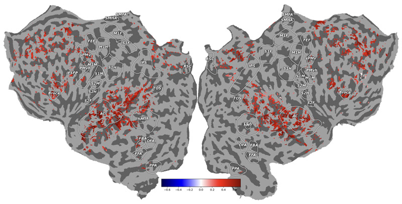
fMRI encoding flatmap
1. Introduction
The comparison of how linguistic representations relate to patterns of brain activity has become an important topic in computational neuroscience and linguistics. Advances in pretrained language models (LMs) have enabled directs comparison between high-dimensional linguistic representations and neural activity measured by functional magnetic resonance imaging (fMRI). In this framework, encoding models predict brain responses from linguistic features, while decoding models reconstruct linguistic content from brain activity 1,2.
Two key methodological choices were explored. First, most studies employ contextual hidden state (HS) representations from intermediate or final layers of LMs, while largely overlooking static input embeddings (IE). HS capture rich syntactic and semantic contexts but are highly variable across occurrences of the same word, raising questions about their alignment with stable lexical-semantic representations in the brain. By contrast, IE are context-invariant and may better reflect stable lexical semantics; however, systematic comparisons of IE and HS across architectures and tasks are lacking.
Second, the dominant mapping approach is linear regression, particularly voxel-wise ridge regression. Although linear models are efficient and interpretable, they may underfit the nonlinear and sequential structures of neural signals. Therefore, sequential neural models have been considered as alternatives in prior studies. For instance, Mittal et al. 3 applied bidirectional long short-term memory (BiLSTMs) to brain-state decoding, showing an approximately 18% improvement in accuracy over unidirectional LSTMs when decoding working memory states. Qiao et al. 4 proposed an approach for visual category decoding using a bidirectional recurrent neural network, inspired by bidirectional cortical information flows. More recently, Kucukosmanoglu et al. 5 used BiLSTMs together with one-dimensional convolutional neural networks for cognitive state classification, and found that BiLSTMs exhibited higher sensitivity to individual performance differences despite slightly lower overall accuracy.
Recent studies have used transformer-based architectures to predict the future resting-state brain activity using extensive datasets. Sun et al. 6 employed a 4D shifted window (Swin) Transformer on human connectome project (HCP) data, using 23.04 s of input fMRI sequences to predict the next 7.2 s of brain states with high spatiotemporal fidelity. Earlier work by Sun et al. 7 also demonstrated that a standard transformer model can accurately forecast up to 5.04 s of brain activity based on the preceding 21.6 s of fMRI, even revealing underlying functional connectivity patterns. Although these findings are promising, they address resting-state prediction tasks and rely on large-scale datasets (e.g., HCP), which provide abundant data for model training. By contrast, our study focused on stimulus-driven brain responses during naturalistic language comprehension and operated under limited-sample conditions. In such settings, transformer models with high parameter counts and strong data requirements are prone to overfitting. Therefore, despite their efficacy in data-rich environments, transformer-based mapping models may not be suitable in our context. BiLSTMs strike a practical balance as sequential baselines, although their utility for naturalistic brain–language modeling has not been systematically evaluated.
Our contributions are threefold:
-
We provide a systematic comparison of IE and HS features across multiple LM architectures in both encoding and decoding tasks.
-
We benchmark linear ridge regression against nonlinear BiLSTM models, test whether sequential nonlinear mappings improve brain–language prediction, and clarify their trade-off with linear interpretability.
-
We present fine-grained voxel-level analyses with explainable variance (EV) normalization, revealing spatial patterns of alignment between stable and context-dependent representations.
3. Dataset
3.1. fMRI Data Acquisition and Preprocessing
We used the publicly available Narratives dataset (OpenNeuro: ds003020) 24,(1) collected at the Biomedical Imaging Center of the University of Texas at Austin. The subjects listened passively to naturalistic spoken stories from the podcast The Moth(2) while undergoing fMRI scanning. MRI was performed using a 3 T Siemens Skyra scanner equipped with a 64-channel head coil. The scanning parameters were as follows: TR = 2 s, TE = 30.8 ms, flip angle = 71°, multiband factor = 2, voxel size = 2.6 mm isotropic, matrix size \(= 84 \times 84\), and field of view = 220 mm, with whole-brain coverage.
Among the 26 available stories, we focused on the narrative “Where There’s Smoke,” which was repeated 10 times for each subject. After excluding the first and last 10 TRs without auditory input, each repetition consisted of \(T=291\) usable TRs. In this study, we analyzed data from three subjects (UTS01–UTS03), each with approximately \(V \approx 81\mbox{,}000\)–95,000 cortical voxels.
Standard preprocessing included motion correction, spatial normalization to a common cortical surface, and \(z\)-scoring of each voxel’s time series. Anatomical scans were defaced for anonymization, and cortical surfaces were reconstructed from T1-weighted images.
3.2. Language Stimuli and Temporal Alignment
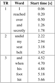
The audio of “Where There’s Smoke” was automatically transcribed using the OpenAI Whisper model 25,(3) followed by manual correction to ensure word-level timing accuracy. Words were then aligned to the fMRI timeline with a resolution of TR \(= 2\) s, producing 291 text segments per repetition. Each TR segment corresponds to words occurring within a 2-s interval. Table 1 shows an example of token alignment for TRs 1–3.
Table 1. Word timing alignment for TRs 1–3 in the story “Where There’s Smoke.” Each TR spans 2 s.
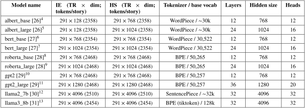
For each TR segment, we extracted linguistic features from multiple pretrained language models (BERT, RoBERTa, ALBERT, GPT-2, and LLaMA). The IE and HS were obtained. Tokens were encoded using each model’s tokenizer, processed in inference mode without gradient updates, and the hidden layer outputs were averaged across the tokens. These yielded feature arrays \(X \in \mathbb{R}^{T \times D}\) that aligned with the fMRI responses \(Y\). A complete list of the models and architectural details is summarized in Table 2.
Table 2. Language models used for feature extraction. For both IE and HS, token-level vectors within each TR are mean-pooled to a TR-level sequence of length \(T=291\). The numbers in parentheses indicate the total number of sub-tokens produced by the tokenizer for our story (tokens/story). Architectural details (layers, hidden size, attention heads) are included for reference.
The story transcript was aligned to the fMRI time axis, with each TR segment indexed by \(t\) (\(t=1,\dots,T\), \(T=291\)) associated with the words spoken during that TR interval.
4. Methods
4.1. Linguistic Feature Extraction
All tokenization, embedding lookups, and hidden-state extractions were implemented using the Hugging Face Transformers library 32 with the corresponding pretrained model tokenizers and model APIs. The variables add_special_tokens, attention_mask, and special_tokens_mask, mentioned below, were obtained directly from this library.
4.1.1. IE Representations
For each model, we obtained the IE, which are token-wise, context-independent representations, by looking up the embedding table using the model’s native tokenizer. Specifically, for a given TR \(t\), we consider its word list \((\text{word}_{t,1},\dots,\text{word}_{t,M_t})\) and tokenize each word independently with add_special_tokens=False. We did not insert any artificial leading spaces for decoder-style tokenizers based on byte-level byte pair encoding (BPE) (e.g., RoBERTa/GPT-2); each word was treated as an independent unit during tokenization. Let \((w_{t,1},\dots,w_{t,N_t})\) be the resulting subword tokens in TR \(t\) (concatenating all words in order), with the embedding vectors \(\mathbf{E}(w_{t,i})\in\mathbb{R}^D\) from model.get_input_embeddings().
We aggregate to the TR level by a simple mean over all subword tokens in the TR:
4.1.2. HS Representations
For HS representations, which are context-dependent, within each TR, we concatenated all words into a single sequence and ran one forward pass with add_special_tokens=True. We then compute a masked mean over the content tokens by intersecting the tokenizer’s attention_mask (pads off) with special_tokens_mask (special symbols off):
At the TR level, these representations yield matrices
4.2. Experimental Design and Modeling
4.2.1. EV and Noise Ceiling
Before fitting the encoding or decoding models, we quantified the signal-to-noise ratio of the voxel responses using EV, also referred to as signal power 33,34,35. Conceptually, EV measures the proportion of response variance that is consistent across repeated presentations of the same stimulus and is thus attributable to the stimulus rather than measurement noise. Following the classical definition introduced by Sahani and Linden 33, EV can be estimated from the across-repetition variance decomposition:
The second term applies Bessel’s correction—that is, using \(N - 1\) (instead of \(N\)) in the denominator—to yield an unbiased estimate of the variance under finite-sample conditions. This adjustment compensates for the loss of one degree of freedom by estimating the mean from the data 36,37,38.
To improve the robustness of our dataset of 10 repetitions, we adopted the split-half procedure described by Hsu et al. 34. Repetitions were divided into odd and even subsets, averaged within each group, and their correlations were computed as follows:
This correlation was then Spearman–Brown corrected:
The corrected value \(\rho_v\) was treated as the noise ceiling of voxel \(v\), representing the maximum predictable variance for a given number of repeats. We further defined EV operationally as the squared correlation between repeated responses under this split-half scheme, in line with the recommendations of Schoppe et al. 35, who emphasize normalized correlation-based estimates for evaluating neural model performance. For subsequent analyses, we restricted our focus to voxels with \(\mathrm{EV} > 0.1\), retaining these as “high-EV voxels.” This practical threshold follows the implementation in the Gallant Lab’s voxel-wise encoding model tutorials 39, where it is used to reduce the influence of noise-dominated voxels and to ensure more stable model fitting. Therefore, most results were reported across the full voxel set and within this high-EV subset, enabling fairer comparisons across models.
4.2.2. Voxel-Wise Ridge Regression
As a linear baseline, we trained voxel-wise ridge regression models, a widely used approach in fMRI encoding and decoding studies 1,2. Two independent directions were considered: an encoding model mapping linguistic features to fMRI responses, and a decoding model mapping fMRI responses back to linguistic features. Both directions were evaluated separately for the IE and HS representations, yielding a complete set of linear baselines.
For each voxel \(v\), ridge regression was defined as:
The modeling pipeline consists of three stages. First, the input features are mean-centered over time without variance scaling. Second, features were temporally expanded with 1–4 TR delays to account for hemodynamic lag. Third, ridge regression was independently fitted for each voxel. The regularization parameter \(\alpha\) was selected automatically by temporal block cross-validation with non-overlapping folds (boundaries at \([0,97,194,291]\)), evaluated over a logarithmic grid of candidate values (\(10^1\)–\(10^{20}\)). For encoding, linguistic features served as predictors and fMRI responses served as targets. For decoding, fMRI responses were predictors, and the target linguistic features were normalized using the mean and variance statistics from the training split and applied consistently to the test split.
The evaluation followed a repeat-split scheme; odd and even repetitions of the story stimulus were averaged separately to yield independent training and testing sets. The performance metrics were defined according to the model direction. For encoding, the voxel-wise Pearson correlation and noise-ceiling-normalized correlation were reported, while raw and normalized \(R^2\) correlations were examined as auxiliary metrics. For decoding, the performance was quantified using the dimension-wise \(R^2\) and cosine similarities between the predicted and ground-truth embeddings. Similar to the BiLSTM, the results were summarized across all voxels/features and restricted to high-reliability subsets (high-EV voxels or high-reliability feature dimensions).
This ridge regression baseline provides a robust linear benchmark against which the nonlinear BiLSTM models are directly compared.
4.2.3. Repeat-Split Data Partitioning
To obtain independent training and test data while maintaining constant stimulus content, we adopted a repeat-split protocol. The 10 repetitions of the same story stimulus were divided into odd and even subsets, and the responses were averaged within each subset to reduce measurement noise.
In the encoding setting, linguistic embeddings served as predictors and fMRI responses served as targets. Both embedding and fMRI signals were partitioned into odd/even splits such that models were trained on one half (odd) and evaluated on the other (even). The final results were averaged across both directions (odd\(\rightarrow\)even and even\(\rightarrow\)odd).
In the decoding setting, averaged fMRI signals from the odd/even splits were used as predictors, whereas target linguistic embeddings remained identical across repetitions, reflecting the fact that the same transcript corresponded to all neural recordings. The models were trained on one half and tested on the other, ensuring that the predictions were generalized across independent neural measurements of the same stimulus.
4.2.4. BiLSTM Model
In addition to the voxel-wise ridge regression baseline, we trained bidirectional LSTM (BiLSTM) models to test whether nonlinear sequential mapping can improve predictive power. Two independent models were trained: an encoding model mapping linguistic features to fMRI responses, and a decoding model mapping fMRI responses back to linguistic features. For a direct comparison, both were trained using the same data partitions as the ridge regression baseline.
All BiLSTM models were trained on overlapping sliding windows of length 32 TRs with a stride 8 rather than on the full 291-TR sequences. This strategy is commonly used in time-series deep learning to transform long sequences into multiple supervised learning examples, thereby increasing the effective sample size and stabilizing training, while reducing the risk of overfitting 40,41.
Each input window was processed using a two-layer BiLSTM with a hidden size of 256 and a dropout \(p=0.1\). The BiLSTM outputs were passed through a two-layer feed-forward projection (linear–ReLU–dropout–linear) to predict the target representation. The weights were initialized using the Xavier uniform initialization.
The training used the AdamW optimizer42 with a learning rate \(10^{-3}\), weight decay \(10^{-4}\), and a cosine annealing learning rate schedule 43 with \(T_{\max}=150\). The models were trained for up to 150 epochs with early stopping (patience \(=15\) epochs) based on the validation loss. A patience value between 10 and 20 is commonly used in practice to allow minor fluctuations while preventing overfitting 44. Mini-batch training was performed using a batch size of 64.
The evaluation followed the same repeat-split scheme as ridge regression; odd and even repetitions of the story stimulus were averaged separately to yield independent training and testing sets. Within the training period, additional temporal block partitioning was applied for validation and early stopping to ensure that no overlapping time segments were used for training and validation.
4.2.5. Performance Metrics Differed by Direction
For encoding, we evaluated voxel-wise Pearson correlation and noise-ceiling-normalized correlation between predicted and observed responses, as encoding predicts time-series voxel responses, where the similarity of temporal patterns is typically assessed with correlation-based measures. In this setting, it is essential to assess whether the predicted responses align with the observed fluctuations in magnitude, thereby making the correlation-based measures appropriate.
For decoding, we evaluated the dimension-wise \(R^2\) and cosine similarities between the predicted and ground-truth linguistic features. Because these targets are high-dimensional embeddings, cosine similarity captures the alignment in a representational space, whereas \(R^2\) measures variance explained across dimensions.
Accordingly, applying the same evaluation criteria across encoding and decoding would be inappropriate because the predicted targets fundamentally differ in nature (time-series voxel signals versus semantic embeddings). As with ridge regression, the results were reported across all voxels/features and restricted to high-reliability subsets (high-EV voxels or high-reliability feature dimensions).
4.3. Evaluation Metrics
To evaluate model performance, we used metrics tailored to the prediction direction.
Encoding models. For each voxel \(v\), the prediction accuracy was quantified using the Pearson correlation coefficient, which is insensitive to linear rescaling and captures the temporal fidelity:
Because different voxels exhibit different repeat reliabilities, we also report the noise-ceiling-normalized correlation to interpret the performance relative to the maximum predictable variance:
Decoding models. For each feature dimension \(d\), we computed the coefficient of determination \(R^2\), which measures the proportion of variance as follows:
Because linguistic feature dimensions were standardized prior to fitting, they directly reflected the absolute prediction accuracy and were directly comparable across dimensions. Unlike voxels, embedding dimensions do not have heterogeneous noise ceilings; therefore, we report raw \(R^2\) rather than normalized values. Additionally, we compute the cosine similarity between the predicted and ground-truth feature vectors, which reflects the directional alignment in a high-dimensional representational space:
Encoding metrics emphasize voxel-level temporal fidelity and report normalized values to account for voxel reliability, whereas decoding metrics emphasize the explained variance and the geometric similarity of reconstructed embeddings, where raw \(R^2\) suffices are due to standardized feature dimensions. The results were reported across both the full set of voxels/features and restricted to high-reliability subsets (EV \(>0.1\) for voxels, high-repeat dimensions for features).
5. EV Analysis
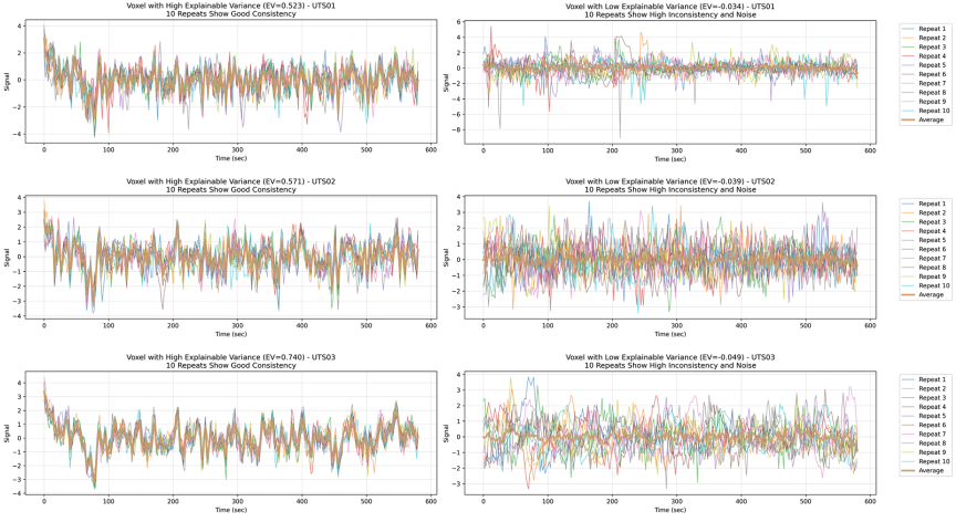
Fig. 1. Examples of voxel-wise signal consistency across repetitions in three subjects (UTS01–UTS03). High-EV voxels (left panels) show high reproducibility across 10 repeated presentations, while low-EV voxels (right panels) show inconsistent, noise-dominated signals.
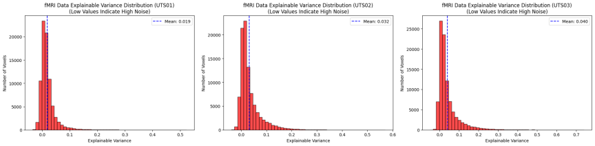
Fig. 2. Voxel-wise EV distributions for each of the three subjects (UTS01–UTS03). The majority of voxels exhibit low EV values (\(<0.05\) to \(0.1\)), reflecting high noise levels in the data.
We first evaluated the reliability of the fMRI dataset using EV, as described in Section 4.2.1. Fig. 1 shows the voxel-wise signal consistency across 10 repetitions in three subjects (UTS01–UTS03). High-EV voxels (left panels) demonstrated strong reproducibility across repetitions, whereas low-EV voxels (right panels) exhibited noisy and inconsistent responses. Fig. 2 summarizes the voxel-wise EV distributions for each participant. The majority of voxels fall below EV thresholds of \(0.05\)–\(0.1\), reflecting high noise levels, whereas only a small fraction of voxels achieve higher EV values.
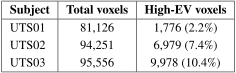
To provide quantitative context, Table 3 reports the number of voxels per subject and the subset of “high-EV” voxels (EV \(>0.1\)). These counts confirm that only a small fraction of voxels is reliable enough to support robust brain–language modeling. Consequently, subsequent analyses were performed on both the full voxel set and high-EV subset.
6. Encoding Results (Features \(\rightarrow\) fMRI)
6.1. Encoding with Voxel-Wise Ridge Regression: IE vs. HS
Table 4 reports encoding performance for both IE and HS across three subjects. As in prior neural encoding work, correlation \(r\) is emphasized as the primary metric, while normalized \(R^2\) is reported for completeness.
For IE, whole-brain correlations were generally low across subjects (\(r \approx 0.056\)–\(0.129\)), confirming that most voxels carry little stimulus-driven signal. By contrast, restricting the analysis to high-EV voxels revealed robust model–brain alignment (\(r \approx 0.318\)–\(0.436\), normalized \(R^2\) up to 0.172), underscoring the necessity of voxel selection.
Across all three subjects, the RoBERTa and GPT-2 embeddings consistently achieved the highest correlations for high-EV voxels (\(r \approx 0.392\)–\(0.436\)), outperforming BERT and ALBERT (\(r \approx 0.318\)–\(0.380\)). LLaMA embeddings showed intermediate correlations (\(r \approx 0.374\)–\(0.419\)), but their normalized \(R^2\) remained strikingly low (\(\approx 0.016\)–\(0.045\)) for all subjects, suggesting weaker unique contributions despite large parameter counts.
Table 3. Voxel counts and number of high-EV voxels (EV \(>0.1\)) for each subject. Percentages indicate the proportion of high-EV voxels relative to the total.
HS representations yielded mixed results compared to IE (\(r \approx 0.157\)–\(0.448\), normalized \(R^2\) up to 0.214). Although HS dramatically improved the performance of BERT, RoBERTa, and ALBERT, this benefit was not observed in the decoder-only architectures.
BERT-base, RoBERTa-large, and ALBERT-base consistently formed the top-performing groups across subjects (\(r \approx 0.395\)–\(0.448\)), surpassing GPT-2-large and RoBERTa-base. By contrast, LLaMA models showed lower correlations compared to their inputs (\(r \approx 0.295\)–\(0.383\)), and GPT-2 (small) dropped substantially (\(r \approx 0.157\)–\(0.177\)), deviating from the pattern observed in BERT/RoBERTa/ALBERT.
Table 4. Encoding with ridge regression. IE and HS are shown side by side (IE/HS). We report correlation \(r\) on all voxels (All) and high-EV voxels (HighEV), and normalized \(R^2\) on HighEV. Bold indicates the highest value, and underline indicates the lowest value for each column. Numbers are per subject (UTS01/02/03).
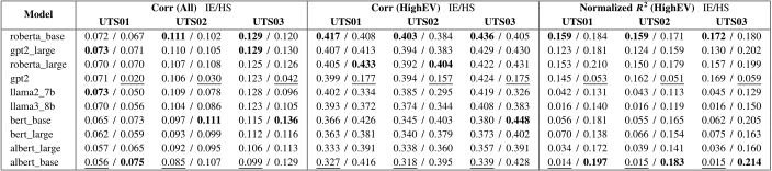
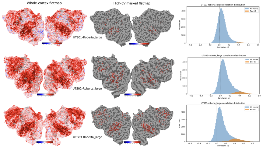
Fig. 3. Cross-subject cortical flatmaps of voxel-wise prediction accuracy using HS features from RoBERTa-large. Each row corresponds to a subject (UTS01–UTS03). Whole-cortex maps (left) show overall correlations, high-EV masked maps (middle) highlight reliable regions, and histograms (right) illustrate the distribution of correlations across voxels. Subjects with higher EV (e.g., UTS03) exhibit broader and stronger predictive regions, demonstrating cross-subject robustness of RoBERTa-large HS representations.
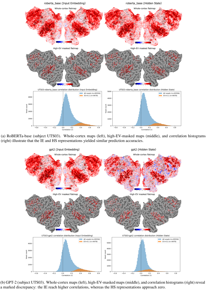
Fig. 4. Comparison of IE and HS representations across models for subject UTS03. (a) RoBERTa-base; (b) GPT-2.
6.2. Flatmap Visualization
To complement the quantitative comparisons in Table 4, we deliberately selected a minimal set of representative models for flatmap visualization in order to highlight the three key patterns while covering both the training objectives and a controllable scale variable.
RoBERTa-large was chosen because it consistently ranked among the top performers across subjects, showing a stable spatial distribution and right-shifted histograms. Therefore, it serves as the most suitable benchmark for cross-subject robustness, allowing readers to immediately observe strong signals in high-EV regions (Fig. 3).
RoBERTa-base, which belongs to the same family and training objective (masked LM) as RoBERTa-large but differs only in scale, provides a typical case in which IE and HS yield comparable performance. This also illustrates that simply scaling up the model size did not qualitatively alter the flatmap patterns. Under the BiLSTM encoding setup, most models converge to a narrow band of high-EV correlations (\(r=0.41\)–0.45 across subjects), with RoBERTa-base/large lying near the center or upper edge of this distribution, ensuring that these choices are representative rather than outliers (Fig. 4).
Finally, GPT-2 exemplifies the autoregressive objective and provides the clearest counterexample. In voxel-wise ridge regression encoding, its embeddings yield reasonably strong predictions whereas its HS produces much weaker predictive performance. Including GPT-2 alongside the RoBERTa models highlights that the training objective and scale can fundamentally change the relative advantage of IE versus HS, rather than reflecting mere numerical fluctuations (Fig. 4).
All three selected models were open-source, widely used, and easy to reproduce. While models such as LLaMA-2 also show “inverted” IE/HS patterns, their behavior overlaps substantially with GPT-2. Given space constraints, we present the results in the tables and discussion, while the figures focus on three representative cases: robust high-performance (RoBERTa-large), typical similarity (RoBERTa-base), and a marked counterexample (GPT-2).
Table 5. Encoding with BiLSTM. Each cell shows IE/HS. We report correlation \(r\) on all voxels (All) and high-EV voxels (HighEV), and normalized \(R^2\) on HighEV. Bold indicates the highest value for each column. Numbers are per subject (UTS01/02/03).
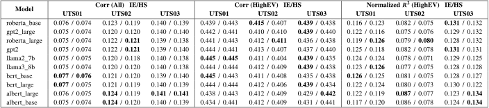
Figure 3 shows the voxel-wise prediction accuracies for the RoBERTa-large HS representations across all three subjects. Each row combines whole-cortex flatmaps, high-EV-masked flatmaps, and correlation histograms. The whole-cortex maps revealed broadly positive correlations, whereas the high-EV-masked maps showed isolated clusters of reliable predictions in the auditory and temporal cortices. Despite individual variability, the spatial pattern of the predictive regions was consistent across subjects, with broader and stronger predictive regions observed in subjects with higher EV (e.g., UTS03).
Figures 4 show the within-subject comparisons between the IE and HS groups. For RoBERTa-base, IE and HS produced nearly identical flatmap patterns and histograms, consistent with their similarly high EV correlations in Table 4. By contrast, GPT-2 (Fig. 4) shows a dramatic inversion: IE yield a right-shifted histogram with many voxels in the \(r=0.3\)–\(0.5\) range, whereas HS representations cluster near zero, producing far fewer predictive voxels. These visualizations underscore that HS representations are not universally superior to IE, and that model-specific factors, such as training objectives and architecture, can fundamentally alter the degree of model-brain alignment.
6.3. Encoding with BiLSTM: IE vs. HS
Table 5 summarizes the encoding performance of the BiLSTM model. Whole-brain correlations remained low across subjects and models (\(r \approx 0.074\)–\(0.141\)), which was consistent with the dominance of noise in most voxels. By contrast, restricting analyses to high-EV voxels revealed robust alignment, with correlations consistently in the range of \(r \approx 0.404\)–\(0.445\) across all subjects and models. The normalized \(R^2\) values reached \(0.134\), further confirming that only a subset of voxels carried reliable stimulus-driven information.
A notable trend is that the differences between IE and HS were minimal under the BiLSTM framework; across all model families, IE and HS achieved nearly identical performance. Moreover, the performance is highly consistent across architectures, with BERT, RoBERTa, GPT-2, ALBERT, and LLaMA clustering within a narrow correlation range. This suggests that the BiLSTM models largely capture the shared temporal dynamics of the fMRI signal, reducing the variance attributable to specific LM architectures or representation types.
6.4. Discussion of Encoding Models
Our encoding analyses showed that meaningful model–brain alignment only emerged after selecting high-EV voxels. Across the entire cortex, the correlations remained close to zero, reflecting the dilution effect of noise-dominated regions. When the analysis is restricted to high-EV voxels, correlations for most models increase substantially into the 0.30–0.45 range, enabling reliable model comparison.
Within high-EV voxels, IE and HS representations perform approximately equivalently on average. For most model families (e.g., BERT, RoBERTa, and ALBERT), HS offers only a slight advantage over IE, and the two are often nearly indistinguishable. This indicates that HS representations are not universally superior to IE; instead, model-specific factors determine alignment outcomes.
Two striking examples highlight this phenomenon. The first is GPT-2 (12 layers, hidden size 768, 12 heads), whose HS performance is extremely poor (\(r \approx 0.157\)–\(0.177\)), despite its IE achieving substantially higher correlations (\(r \approx 0.394\)–\(0.424\)). By contrast, GPT-2 large (36 layers, hidden size 1280, 20 heads) recovered a strong HS performance comparable to BERT and RoBERTa. This suggests that small-scale GPT-2 lacks sufficient capacity to overcome the autoregressive bias of its training objective, producing only shallow continuation signals that fail to align with fMRI; increasing the scale partly compensates for this limitation. Importantly, this weakness cannot be explained by model size alone; other models of comparable capacity (BERT-base, RoBERTa-base, and ALBERT-base; all with 12 layers and a hidden size of approximately 768) achieved strong HS performance, underscoring the decisive role of the training objective—bidirectional masked word recovery versus unidirectional left-to-right prediction.
The second counterexample is LLaMA-2, which exhibits the opposite pattern. Its IE rank is among the strongest of all the models, comparable to RoBERTa-base and GPT-2; however, its HS falls to the bottom tier. This inversion suggests that LLaMA-2’s contextualization process introduces features that are less aligned with cortical signals, possibly because its autoregressive training objective is biased toward local next-word prediction rather than the temporally integrated semantics captured by fMRI. The effect may be magnified by scale; with 32 layers and a hidden size of 4,096, a large proportion of the hidden dimensions may encode syntactic or generative control signals that do not directly map onto brain representations.
Finally, the EV at the subject level appeared to influence the attainable ceiling; subjects such as UTS03 tended to reach slightly higher maximum correlations. However, the cross-subject model rankings remained largely stable, with RoBERTa, BERT, and ALBERT forming the top tier, GPT-2 large often close behind, and GPT-2 small and LLaMA-2 consistently at the bottom.
Beyond the choice of language model features, the mapping model itself plays a crucial role. In a parallel analysis, we compared the linear ridge regression used in this study with a nonlinear BiLSTM model. Although BiLSTM yielded modest but consistent performance gains, we found that the simpler linear model served as a more effective probe for revealing fine-grained representational differences between language models. The more powerful BiLSTM, in its capacity to learn general temporal structures in the fMRI signal, tended to compress these inter-model differences, making them more difficult to distinguish. This highlights a critical trade-off for future neuro-AI research: maximizing predictive accuracy with complex nonlinear models versus achieving clearer representational interpretability with simpler linear models.
In summary, these findings highlight three points: (i) voxel selection is essential; (ii) within high-EV voxels, IE and HS provide broadly comparable predictivity; and (iii) model-specific factors such as training objective, architecture, and scale can overturn expected trends, as exemplified by GPT-2 and LLaMA-2.
7. Decoding Results (fMRI \(\rightarrow\) Features)
7.1. Decoding with Ridge Regression: IE vs. HS
We report the decoding results for all three subjects in Table 6. This table summarizes \(R^2\) and cosine similarity scores for both IE and HS representations, evaluated on full-brain voxels as well as on high-EV voxels.
Table 6. Decoding with ridge regression (fMRI \(\to\) language features) with mixed vertical layout. Each cell shows IE/HS. We report \(R^2\) and cosine similarity (CosSim) for full-brain and high-EV voxels. Bold indicates the highest value for each column. Numbers are per subject (UTS01/02/03).
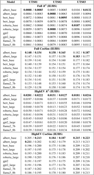
Across all three subjects, the decoding performance on the full voxel set was modest, which was consistent with the large proportion of noise-dominated voxels. By contrast, restricting the analysis to high-EV voxels generally improved both \(R^2\) and the cosine similarity across subjects and models, indicating that stimulus-sensitive regions carry more recoverable lexical information. This trend can be observed in many model–subject pairs, as shown in Table 6. For example, ALBERT-base achieved \(R^2 = 0.0201\) and a cosine similarity of \(= 0.205\) in UTS01; \(R^2 = 0.0216\) and cosine similarity \(= 0.223\) in UTS03 under a high-EV setting.
When comparing feature types, HS shows clearer advantages over IE in high-EV settings. This pattern is especially evident in UTS01 and UTS03 across both \(R^2\) and CosSim, whereas UTS02 exhibits more mixed behavior depending on the model. These gains were consistent across many models, indicating that contextualization can improve predictive alignment in stimulus-sensitive regions. However, this advantage is not universal. For instance, ALBERT-large shows cases in which IE matches or even exceeds HS (UTS01/02), underscoring that contextual features do not guarantee superior alignment across all architectures.
7.2. Decoding with BiLSTM: IE vs. HS
Table 7. Decoding with BiLSTM (fMRI \(\to\) language features). Each cell shows IE/HS. We report \(R^2\) and cosine similarity (CosSim) for full-brain and high-EV voxels. Bold indicates the highest value for each column. Numbers are per subject (UTS01/02/03).
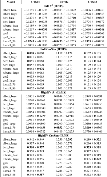
Table 7 summarizes the decoding performance using the BiLSTM models for the three subjects. In the full voxel set, the \(R^2\) values were consistently negative across all models, indicating that noise-dominated regions obscured reliable mapping. Nevertheless, the cosine similarity scores remained positive, suggesting that BiLSTM captures some coarse directional structures in the reconstructed feature space, even when the variance explanation is poor. When restricted to high-EV voxels, performance improved substantially. These values are markedly higher than those observed using ridge regression, confirming that BiLSTM leverages temporal dependencies to improve decoding in reliable cortical regions.
Comparing the feature types, HS and IE performed similarly under BiLSTM. Unlike the ridge regression results, where HS often has a clear advantage, the gap between IE and HS largely disappears here; in many cases, the two are nearly identical, and in some instances, IE even slightly outperforms HS (e.g., LLaMA-2 in UTS02/03). This convergence suggests that the nonlinear sequential modeling of BiLSTM reduces the relative contribution of contextualization, making static embeddings nearly as effective as HS.
Overall, the BiLSTM decoder provides clear gains over ridge regression in high-EV voxels but at the cost of compressing the distinctions between the LM feature types. This indicates that, while nonlinear sequence models enhance predictive power in reliable regions, they may obscure representational differences that are more apparent in linear mappings.
7.3. Discussion of Decoding Models
The decoding results revealed a clear contrast between the linear ridge regression and the nonlinear BiLSTM models.
With ridge regression (Table 6), the performance on the full voxel set was weak but still positive, and improved modestly on high-EV voxels. These values indicate that linear mappings capture some recoverable lexical-level structures, but are strongly limited by noise in the fMRI signals.
By contrast, BiLSTM decoding (Table 7) produced negative \(R^2\) values for the full voxel set. Such negative values arise when unreliable voxels are dominated by noise, causing the nonlinear models to overfit spurious patterns and perform worse than a trivial mean baseline. This contrast indicates that obtaining positive values for high-EV voxels is meaningful. EV filtering removes noise-dominated regions and is consistent with the benefits of temporal sequence modeling in reliable cortical areas.
The relationship between IE and HS also differed between the mapping models. Under ridge regression, HS is typically superior to IE. By contrast, BiLSTM decoding largely eliminates this gap; IE and HS achieve nearly identical scores, and in several cases, IE slightly surpasses HS. This suggests that BiLSTM sequential modeling reduces the unique contribution of contextual features, making static embeddings nearly as effective as HS for reconstructing language features from brain activity.
Collectively, these findings highlight a critical methodological trade-off. Ridge regression provides stable, interpretable baselines that preserve differences between LM feature types, whereas BiLSTM offers stronger predictive accuracy in high-reliability regions but compresses inter-model and IE–HS distinctions. For decoding, the choice between linear and nonlinear models reflects a balance between maximizing predictive performance and maintaining representational interpretability.
8. Methodological Limitations
8.1. Mapping Models and Neural Mechanisms
The encoding and decoding models used in this study (ridge regression and BiLSTM) should be understood as statistical mapping tools rather than models of neural computation. These approaches quantify correspondences between linguistic representations and brain activity patterns but do not explain the physiological mechanisms by which the brain processes language.
The human brain involves extensive recurrent circuits, feedback loops, and large-scale interactions across regions that are far more complex than the feedforward architecture used in this study. Accordingly, the current findings concern representational alignment under the encoding/decoding framework rather than mechanistic explanations of language processing in the brain.
8.2. Passive Language Comprehension Paradigm
The fMRI paradigm used in this study was based on passive language comprehension, in which participants listened to or read continuous narrative stimuli. This setup primarily captured the perceptual and semantic aspects of language processing.
In natural settings, however, human language involves active cognitive functions such as reasoning, planning, memory retrieval, and emotional simulation. These higher-order processes were not the primary focus of the experimental design. Therefore, the present results should be interpreted within the scope of passive comprehension rather than active language use.
8.3. Memory and Experience in Language Understanding
The observed alignment reflects the representational similarity between LM-derived linguistic features and fMRI responses. This finding should not be interpreted as evidence that language models capture memory-based or experience-based interpretation processes in the human brain.
Human language understanding relies heavily on episodic memory, world knowledge, and embodied experience, engaging regions beyond the core language network, such as the hippocampus and the prefrontal cortex. By contrast, representations extracted from language models reflect statistical regularities learned from text corpora rather than grounded experiential knowledge.
8.4. Prediction and Reasoning in Narrative Comprehension
The present findings examine the spatial alignment between linguistic representations and cortical activity during passive comprehension. They do not address the dynamic mechanisms underlying human prediction or reasoning.
While language models perform next-word prediction based on statistical regularities, human prediction during narrative comprehension relies on the integration of memory, world knowledge, and reasoning processes involving distributed brain networks and dynamic interactions over time. Accordingly, the cortical distributions reported here should be interpreted as reflecting representational encoding rather than active prediction or reasoning.
9. Conclusion
This study provides a systematic comparison of IE and HS representations from multiple large language model families in both encoding and decoding frameworks. Using voxel-wise ridge regression and nonlinear BiLSTM models, we examined how different feature types and mapping approaches aligned with fMRI signals across three subjects.
Our findings highlighted three key points. First, IE and HS often achieve comparable performances, with HS showing advantages in many high-EV conditions, indicating that both stable lexical semantics and contextualized representations are relevant for modeling brain activity. Second, the choice of mapping model strongly shapes the observed conclusions: ridge regression offers clear and interpretable comparisons that preserve differences across model families and representation types, whereas BiLSTM provides substantial performance gains in high-EV voxels but tends to reduce distinctions between IE and HS, as well as across model families. Third, the contrast between linear and nonlinear mappings highlights difference between encoding and decoding; while the encoding performance remains relatively stable across mapping models, the decoding performance improves markedly under BiLSTM once unreliable voxels are excluded.
Together, these results suggest that progress in neuro-AI modeling requires careful consideration of the methodological role of the mapping model, as the optimal choice depends on the research objective. Linear ridge regression provides stable and quantitatively precise estimates that are well-suited for the comparative scientific analysis of representations. By contrast, nonlinear sequence models, such as BiLSTM, can substantially improve the predictive performance in decoding when restricted to reliable cortical regions. Future work may seek to combine the strengths of both approaches—using nonlinear models for predictive performance while relying on linear models for interpretability and fine-grained regional comparisons—and to extend the analysis to multimodal or generative brain–language decoding frameworks.
Acknowledgments
This work was supported by JST SPRING, Japan (Grant Number JPMJSP2181), and Research Grant (C) from the Tateisi Science and Technology Foundation.
Footnotes
(1) https://openneuro.org/datasets/ds003020 [Accessed September 1, 2025]
(2) https://themoth.org/podcast [Accessed September 1, 2025]
(3) https://huggingface.co/openai/whisper-large-v3 [Accessed September 1, 2025]
(4) https://huggingface.co/albert/albert-base-v2 [Accessed September 1, 2025]
(5) https://huggingface.co/albert/albert-large-v2 [Accessed September 1, 2025]
(6) https://huggingface.co/google-bert/bert-base-uncased [Accessed September 1, 2025]
(7) https://huggingface.co/google-bert/bert-large-uncased [Accessed September 1, 2025]
(8) https://huggingface.co/FacebookAI/roberta-base [Accessed September 1, 2025]
(9) https://huggingface.co/FacebookAI/roberta-large [Accessed September 1, 2025]
(10) https://huggingface.co/openai-community/gpt2 [Accessed September 1, 2025]
(11) https://huggingface.co/openai-community/gpt2-large [Accessed September 1, 2025]
(12) https://huggingface.co/meta-llama/Llama-2-7b [Accessed September 1, 2025]
(13) https://huggingface.co/meta-llama/Meta-Llama-3-8B [Accessed September 1, 2025]
- [1] T. Naselaris, K. N. Kay, S. Nishimoto, and J. L. Gallant, “Encoding and decoding in fMRI,” NeuroImage, Vol.56, No.2, pp. 400-410, 2011. https://doi.org/10.1016/j.neuroimage.2010.07.073
- [2] A. G. Huth, S. Nishimoto, A. T. Vu, and J. L. Gallant, “A continuous semantic space describes the representation of thousands of object and action categories across the human brain,” Neuron, Vol.76, No.6, pp. 1210-1224, 2012. https://doi.org/10.1016/j.neuron.2012.10.014
- [3] A. Mittal, P. Aggarwal, L. Pessoa, and A. Gupta, “Robust Brain State Decoding Using Bidirectional Long Short Term Memory Networks in functional MRI,” bioRxiv, 2021. https://doi.org/10.1101/2021.06.18.449069
- [4] K. Qiao, J. Chen, L. Wang, C. Zhang, L. Zeng, L. Tong, and B. Yan, “Category Decoding of Visual Stimuli From Human Brain Activity Using a Bidirectional Recurrent Neural Network to Simulate Bidirectional Information Flows in Human Visual Cortices,” Frontiers in Neuroscience, Vol.13, Article No.692, 2019. https://doi.org/10.3389/fnins.2019.00692
- [5] M. Kucukosmanoglu, J. O. Garcia, J. Brooks, and K. Bansal, “Influence of cognitive networks and task performance on fMRI-based state classification using DNN models,” Scientific Reports, Vol.15, No.1, Article No.23689, 2025. https://doi.org/10.1038/s41598-025-05690-x
- [6] Y. Sun, D. Chahine, Q. Wen, T. Liu, X. Li, Y. Yuan, F. Calamante, and J. Lv, “Voxel-Level Brain States Prediction Using Swin Transformer,” IEEE J. of Biomedical and Health Informatics, Vol.29, No.12, pp. 8719-8726, 2025. https://doi.org/10.1109/JBHI.2025.3613793
- [7] Y. Sun, M. Cabezas, J. Lee, C. Wang, W. Zhang, F. Calamante, and J. Lv, “Predicting Human Brain States with Transformer,” A. Schroder et al. (Eds.), “Medical Image Computing and Computer Assisted Intervention – MICCAI 2024 Workshops,” pp. 136-146, Springer Nature Switzerland, 2025. https://doi.org/10.1007/978-3-031-84525-3_12
- [8] M. Toneva and L. Wehbe, “Interpreting and improving natural-language processing (in machines) with natural language-processing (in the brain),” Advances in Neural Information Processing Systems, Vol.32, 2019.
- [9] M. Schrimpf, I. A. Blank, G. Tuckute, C. Kauf, E. A. Hosseini, N. Kanwisher, J. B. Tenenbaum, and E. Fedorenko, “The neural architecture of language: Integrative modeling converges on predictive processing,” Proc. of the National Academy of Sciences, Vol.118, No.45, Article No.e2105646118, 2021. https://doi.org/10.1073/pnas.2105646118
- [10] C. Caucheteux and J.-R. King, “Brains and algorithms partially converge in natural language processing,” Communications Biology, Vol.5, No.1, Article No.134, 2022. https://doi.org/10.1038/s42003-022-03036-1
- [11] M. E. Peters, M. Neumann, M. Iyyer, M. Gardner, C. Clark, K. Lee, and L. Zettlemoyer, “Deep contextualized word representations,” arXiv preprint, arXiv:1802.05365, 2018. https://doi.org/10.48550/arXiv.1802.05365
- [12] M. Liu and I. Kobayashi, “Do Feature Representations from Different Language Models Affect Accuracy of Brain Encoding Models’ Predictions?,” 2024 IEEE Int. Conf. on Systems, Man, and Cybernetics (SMC), pp. 2766-2771, 2024. https://doi.org/10.1109/SMC54092.2024.10831584
- [13] R. Antonello, A. Vaidya, and A. G. Huth, “Scaling laws for language encoding models in fMRI,” Advances in Neural Information Processing Systems, Vol.36, pp. 21895-21907, 2023.
- [14] J. Tang, M. Du, V. A. Vo, V. Lal, and A. G. Huth, “Brain encoding models based on multimodal transformers can transfer across language and vision,” Proc. of the 37th Int. Conf. on Neural Information Processing Systems (NIPS ’23), 2023.
- [15] S. R. Oota, Z. Chen, M. Gupta, R. S. Bapi, G. Jobard, F. Alexandre, and X. Hinaut, “Deep Neural Networks and Brain Alignment: Brain Encoding and Decoding (Survey),” arXiv preprint, arXiv:2307.10246, 2024. https://doi.org/10.48550/arXiv.2307.10246
- [16] T. D. la Tour, M. Eickenberg, A. O. Nunez-Elizalde, and J. L. Gallant, “Feature-space selection with banded ridge regression,” NeuroImage, Vol.264, Article No.119728, 2022. https://doi.org/https://doi.org/10.1016/j.neuroimage.2022.119728
- [17] N. Affolter, B. Egressy, D. Pascual, and R. Wattenhofer, “Brain2Word: Decoding Brain Activity for Language Generation,” arXiv preprint, arXiv:2009.04765, 2020. https://doi.org/10.48550/arXiv.2009.04765
- [18] J. Tang et al., “Semantic reconstruction of continuous language from non-invasive brain recordings,” Nature Neuroscience, Vol.26, pp. 858-866, 2023. https://doi.org/10.1038/s41593-023-01304-9
- [19] P. Liu, G. Dong, D. Guo, K. Li, F. Li, X. Yang, M. Wang, and X. Ying, “A Survey on fMRI-based Brain Decoding for Reconstructing Multimodal Stimuli,” arXiv preprint, arXiv:2503.15978, 2025. https://doi.org/10.48550/arXiv.2503.15978
- [20] A. Goldstein, A. Grinstein-Dabush, M. Schain, H. Wang, Z. Hong, B. Aubrey, S. A. Nastase, Z. Zada, E. Ham, A. Feder et al., “Alignment of brain embeddings and artificial contextual embeddings in natural language points to common geometric patterns,” Nature Communications, Vol.15, No.1, Article No.2768, 2024. https://doi.org/10.1038/s41467-024-46631-y
- [21] L. Zhao, Z. Wu, H. Dai, Z. Liu, X. Hu, T. Zhang, D. Zhu, and T. Liu, “A generic framework for embedding human brain function with temporally correlated autoencoder,” Medical Image Analysis, Vol.89, Article No.102892, 2023. https://doi.org/https://doi.org/10.1016/j.media.2023.102892
- [22] H. Li and Y. Fan, “Interpretable, highly accurate brain decoding of subtly distinct brain states from functional MRI using intrinsic functional networks and long short-term memory recurrent neural networks,” NeuroImage, Vol.202, Article No.116059, 2019. https://doi.org/10.1016/j.neuroimage.2019.116059
- [23] S. Ma, L. Wang, L. Hou, S. Hou, and B. Yan, “An fMRI visual neural encoding method with multimodal large language model,” Knowledge-Based Systems, Vol.326, Article No.114049, 2025. https://doi.org/10.1016/j.knosys.2025.114049
- [24] A. LeBel, L. Wagner, S. Jain, A. Adhikari-Desai, B. Gupta, A. Morgenthal, J. Tang, L. Xu, and A. G. Huth, “A natural language fMRI dataset for voxelwise encoding models,” Scientific Data, Vol.10, No.1, Article No.555, 2023. https://doi.org/10.1038/s41597-023-02437-z
- [25] A. Radford, J. W. Kim, T. Xu, G. Brockman, C. McLeavey, and I. Sutskever, “Robust Speech Recognition via Large-Scale Weak Supervision,” arXiv preprint, arXiv:2212.04356, 2022. https://doi.org/10.48550/arXiv.2212.04356
- [26] Z. Lan, M. Chen, S. Goodman, K. Gimpel, P. Sharma, and R. Soricut, “ALBERT: A Lite BERT for Self-supervised Learning of Language Representations,” arXiv preprint, arXiv:1909.11942, 2019. https://doi.org/10.48550/arXiv.1909.11942
- [27] J. Devlin, M.-W. Chang, K. Lee, and K. Toutanova, “BERT: Pre-training of Deep Bidirectional Transformers for Language Understanding,” arXiv preprint, arXiv:1810.04805, 2018. https://doi.org/10.48550/arXiv.1810.04805
- [28] Y. Liu, M. Ott, N. Goyal, J. Du, M. Joshi, D. Chen, O. Levy, M. Lewis, L. Zettlemoyer, and V. Stoyanov, “RoBERTa: A Robustly Optimized BERT Pretraining Approach,” arXiv preprint, arXiv:1907.11692, 2019. https://doi.org/10.48550/arXiv.1907.11692
- [29] A. Radford, J. Wu, R. Child, D. Luan, D. Amodei, and I. Sutskever, “Language models are unsupervised multitask learners,” OpenAI Blog, 2019.
- [30] H. Touvron, L. Martin, K. Stone, P. Albert, A. Almahairi, Y. Babaei, N. Bashlykov, S. Batra, P. Bhargava, S. Bhosale et al., “Llama 2: Open Foundation and Fine-Tuned Chat Models,” arXiv preprint, arXiv:2307.09288, 2023. https://doi.org/10.48550/arXiv.2307.09288
- [31] A. Grattafiori et al., “The Llama 3 Herd of Models,” 2024. LLaMA 3.1-8B model: https://huggingface.co/meta-llama/Llama-3.1-8B [Accessed March 20, 2025]
- [32] T. Wolf, L. Debut, V. Sanh, J. Chaumond, C. Delangue, A. Moi, P. Cistac, T. Rault, R. Louf, M. Funtowicz, J. Davison, S. Shleifer, P. von Platen, C. Ma, Y. Jernite, J. Plu, C. Xu, T. Le Scao, S. Gugger, M. Drame, Q. Lhoest, and A. Rush, “Transformers: State-of-the-Art Natural Language Processing,” Proc. of the 2020 Conf. on Empirical Methods in Natural Language Processing: System Demonstrations, pp. 38-45, 2020. https://doi.org/10.18653/v1/2020.emnlp-demos.6
- [33] M. Sahani and J. F. Linden, “How Linear are Auditory Cortical Responses?,” Advances in Neural Information Processing Systems, Vol.15, 2002.
- [34] A. Hsu, A. Borst, and F. E. Theunissen, “Quantifying variability in neural responses and its application for the validation of model predictions,” Network: Computation in Neural Systems, Vol.15, No.2, pp. 91-109, 2004. https://doi.org/10.1088/0954-898X/15/2/002
- [35] O. Schoppe, N. S. Harper, B. D. B. Willmore, A. J. King, and J. W. H. Schnupp, “Measuring the performance of neural models,” Frontiers in Computational Neuroscience, Vol.10, Article No.10, 2016. https://doi.org/10.3389/fncom.2016.00010
- [36] F. Reichel, “On Bessel’s Correction: Unbiased Variance, Degrees of Freedom, and the Sum of Pairwise Differences,” Qeios, 2025. https://doi.org/10.32388/3GJGNA
- [37] W. J. Reichmann, “The Use and Abuse of Statistics,” Oxford University Press, 1961.
- [38] G. Upton and I. Cook, “A Dictionary of Statistics, 2nd ed.,” Oxford University Press, 2008.
- [39] A. G. Huth and G. Lab, “Voxelwise encoding model (VEM) tutorials,” 2021. https://gallantlab.org/voxelwise_tutorials/ [Accessed September 10, 2025]
- [40] J. Brownlee, “Deep Learning for Time Series Forecasting: Predict the Future with MLPs, CNNs and LSTMs in Python,” Machine Learning Mastery, 2018.
- [41] Data Science StackExchange, “Sliding window leads to overfitting in LSTM?,” 2018. https://datascience.stackexchange.com/questions/27628/ [Accessed September 10, 2025]
- [42] I. Loshchilov and F. Hutter, “Decoupled Weight Decay Regularization,” Proc. of the Int. Conf. on Learning Representations (ICLR), 2019.
- [43] I. Loshchilov and F. Hutter, “SGDR: Stochastic Gradient Descent with Warm Restarts,” Proc. of the Int. Conf. on Learning Representations (ICLR), 2017.
- [44] L. Prechelt, “Early Stopping – But When,?” G. B. Orr and K.-R. Müller (Eds.), “Neural Networks: Tricks of the Trade," Lecture Notes in Computer Science, Vol.1524, pp. 55-69, Springer, 1998. https://doi.org/10.1007/3-540-49430-8_3
This article is published under a Creative Commons Attribution-NoDerivatives 4.0 Internationa License.