
Research Paper:
Improvement Target Identification in Ratio-Based Data Envelopment Analysis: A Novel Methodological Approach
Xu Wang*,†
 , Hiroki Iwamoto**
, and Takashi Hasuike***
, Hiroki Iwamoto**
, and Takashi Hasuike***
*Faculty of Informatics, Gunma University
4-2 Aramakicho, Maebashi, Gunma 371-8510, Japan
†Corresponding author
**Graduate School of International Social Sciences, Yokohama National University
79-4 Tokiwadai, Hodogaya-ku, Yokohama 240-8501, Japan
***Department of Industrial and Management Systems Engineering, Waseda University
3-4-1 Okubo, Shinjuku-ku, Tokyo 169-8555, Japan

The DEA-R model, which integrates data envelopment analysis (DEA) with ratio analysis, allows for the evaluation of efficiency using ratio data. One main strength of DEA is its ability to provide concrete improvement targets for inefficient decision-making units (DMUs). However, identifying these targets within the DEA-R framework is particularly challenging because of the inherent characteristics of ratio data. To address this issue, this study proposes a novel approach for identifying concrete improvement targets for inputs or outputs within the DEA-R framework. Specifically, we construct the DEA-R efficient frontier based on a unique concept and develop an approach to identify improvement targets that lie explicitly on this frontier. This ensures that all the identified targets are DEA-R efficient, thereby guaranteeing their rationality and validity. Furthermore, the constructed frontier enables the setting of flexible improvement targets under various scenarios, thereby enhancing the practicality and adaptability of the proposed approach.
1. Introduction
With economic globalization, improving organizational efficiency has become essential across all sectors and countries. Since its introduction by Charnes et al. 1, data envelopment analysis (DEA) has been widely used to evaluate the relative efficiency of multi-input, multi-output organizations—known as decision-making units (DMUs)—in fields such as education, banking, and healthcare. DEA not only determines whether a DMU is efficient but also provides efficiency scores and concrete improvement targets for inefficient DMUs. However, although conventional DEA models can rank DMUs and suggest improvement targets for inputs and outputs, they are not designed to handle ratio data (for example, return on assets) that are common and important in many practical applications. To address this limitation, DEA-R models have been developed by integrating DEA with ratio analysis.
DEA-R models, which are applicable to real-world data in the form of ratios,(1) have gained significant attention since the initial proposals by Despić et al. 4. Thus, these models have been advanced both theoretically and practically. Notable variants include DEA-R models 5,6,7,8 based on the conventional Charnes-Cooper-Rhodes (CCR) 1 and Banker-Charnes-Cooper (BCC) 9 models, slack-based DEA-R models 10,11, and DEA-R models capable of handling negative data 12. Additionally, with the growing interest in network DEA frameworks, several DEA-R models have been proposed for evaluating the efficiency of these structures involving ratio data. Examples include network DEA-R applications for evaluating the efficiency of banks 13,14, non-life insurance companies 15, and the supply chains of public hospitals 16. Although DEA-R models have proven effective for evaluating efficiency, approaches for identifying improvement targets remain underdeveloped. Conventional DEA models offer various mechanisms for improvement target identifying; for example, the CCR and BCC models improve inputs or outputs, whereas the range-adjusted measure (RAM) 17 and slacks-based measure (SBM) 18 models focus on slack-based improvements to both inputs and outputs. In addition, shortest-distance DEA models 19,20,21 have recently gained attention for offering minimal and practical improvement paths.
Based on the foregoing, this study aims to develop an approach to identifying improvement targets within the DEA-R framework. Because of the nature of the ratio data in DEA-R (for example, \({y}/{x}\) and \({x}/{y}\), where a single input or output simultaneously contributes to multiple ratios), specifying concrete improvement targets for inputs and outputs is difficult, as is commonly performed in conventional DEA. This makes identifying improvement target particularly challenging in DEA-R. Few methods exist for identifying improvement targets, and the identified targets rarely lie on the DEA-R efficient frontier; thus, their efficiency is not guaranteed. For instance, Mozaffari et al. 8 proposed a central resource allocation model based on DEA-R to provide input and output improvement targets for inefficient DMUs. However, when these input and output improvement targets are converted into ratio indicators, they become inefficient, violating the principles of DEA-R efficiency. In DEA and DEA-R, improvement targets are generally expected to lie on the efficient frontier. If this condition is not satisfied, the validity and rationality of the improvement targets are questionable. In addition, Mozaffari et al. 22 proposed an approach for identifying efficient surfaces in DEA-R, and Mozaffari et al. 23 developed a benchmark identification approach. However, neither addressed the issue of identifying concrete improvement targets.
Therefore, this study aims to develop an approach that satisfies the following two properties:
-
(1)
Provide concrete improvement targets for either inputs or outputs.
-
(2)
Ensure that the identified targets are DEA-R efficient.
To this end, we construct the efficient frontier based on a novel concept tailored for ratio data. Building on this, we propose an approach that redefines the conventional target-identification process and ensures that the identified targets lie directly on the constructed efficient frontier. This guarantees that all targets are DEA-R efficient, thereby ensuring their validity and rationality. Furthermore, the availability of the constructed frontier allows for scenario-based target identifaication, thereby enhancing the flexibility and practical utility of the proposed approach. Thus, the proposed approach offers a reliable and effective solution for improvement of target identification in DEA-R, contributing to the further development of this line of research.
The remainder of this paper is organized as follows: Section 2 introduces the key concepts and the formulation of the DEA-R model. Section 3 describes the framework of the proposed approach. Section 4 presents the results of numerical experiments used to demonstrate the effectiveness of the proposed approach. Finally, Section 5 concludes the study and outlines potential future research directions.
2. Preliminaries
Let there be \(n\) DMUs. Each DMU\(_j~(j =1,2,\dots,n)\) uses \(m\) inputs \(\boldsymbol{x}_j = (x_{1j}, x_{2j}, \dots , x_{ij}, \dots , x_{mj})^\top > 0\) to produce \(s\) outputs \(\boldsymbol{y}_j =(y_{1j}, y_{2j}, \dots , y_{rj}, \dots, y_{sj}) > 0\). The \(n\) denotes the total number of DMUs, and the subscript \(j\) represents the \(j\)-th DMU. The subscript \(m\) represents the total number of inputs, and \(i\) denotes an arbitrary input index. Similarly, the subscript \(s\) represents the total number of outputs, and \(r\) denotes an arbitrary output index. The symbol \(s\) is also used to denote slack variable, and the symbol \(r\) is also used to denote the ratio indicator that are defined in the notation list below. The notations used in this study are summarized as follows:
-
\({x}_{ij}\): the \(i\)-th input data of DMU\(_j\) (\(i = 1, 2, \dots, m\))
-
\(\boldsymbol{x}_j\): the input data vector of DMU\(_j\)
-
\({y}_{rj}\): the \(r\)-th output data of DMU\(_j\) (\(r = 1, 2, \dots, s\))
-
\(\boldsymbol{y}_j\): the output data vector of DMU\(_j\)
-
\(\displaystyle r^{ri}_j={y_{rj}}/{x_{ij}}\): the output-to-input ratio indicator constructed by \({x}_{ij}\) and \({y}_{rj}\)
-
The vector of output-to-input ratio indicator
\begin{align*} \boldsymbol{r}_j &= \big(r^{11}_j, r^{12}_j, \dots , r^{1m}_j, \\ &\phantom{=~}~~~r^{21}_j, r^{22}_j, \dots ,r^{2m}_j, \\ &\phantom{=~}~~~\dots ,\\ &\phantom{=~}~~~r^{s1}_j, r^{s2}_j, \dots , r^{sm}_j\big)^\top \end{align*} -
\(R= (\boldsymbol{r}_1, \boldsymbol{r}_2, \dots , \boldsymbol{r}_n)\): the matrix of the output-to-input ratio indicator. In this study, model formulations and methodological developments are presented based on the output-to-input ratio indicator. Notably, the proposed approach is also applicable to the input-to-output ratio indicator.
-
\(R_E= (\boldsymbol{r}_1, \boldsymbol{r}_2, \dots , \boldsymbol{r}_n)\): the matrix of the output-to-input ratios for efficient DMUs
-
\(\symbf{\lambda} =(\lambda_1,\lambda_2,\dots,\lambda_n)^\top\): the weight vector of each DMU
-
\(\boldsymbol{1}\) represents a vector for which all the elements have a value of one, and \(\boldsymbol{0}\) denotes a zero vector.
-
DMU\(_o\): the DMU under evaluation
-
\(s^{ri}\): the slack corresponding to the output-to-input indicator \(r^{ri}\)
-
The slack vector of the output-to-input ratio indicator slack vector:
\begin{align*} \boldsymbol{s} &= \big(s^{11}, s^{12}, \dots, s^{1m},\\ &\phantom{=~}~~~s^{21}, s^{22}, \dots ,s^{2m},\\ &\phantom{=~}~~~\dots ,\\ &\phantom{=~}~~~s^{s1}, s^{s2}, \dots , s^{sm}\big)^\top \end{align*}
The production possibility set in DEA-R can be defined as follows:
3. Proposal of the Methodological Approach
3.1. Concept Behind the Proposed Approach
This study proposes an approach based on output-to-input ratio indicators, which can also be extended to input-to-output ratio indicators. To ensure generalizability, all possible combinations of outputs and inputs are considered. DEA users can specify their desired output-to-input combinations to construct the necessary ratio-based indicators. The proposed approach identifies concrete improvement targets for outputs while maintaining the inputs constant. Therefore, improvement targets are presented as concrete output values to ensure their practical applicability. When these targets are converted into ratio indicators, they are guaranteed to be efficient. Because the proposed approach operates within the DEA-R framework, DEA-R efficiency is ensured, thereby validating the rationality and appropriateness of improvement targets. To achieve these objectives, the proposed approach for identifying improvement targets in DEA-R is developed based on the following three key ideas and procedures.
-
Calculate the efficient DMUs within the given set \(\boldsymbol{R}\) by model 2.
-
Construct \(E_\text{R}\) using the calculated efficient DMUs as follows:
\begin{align} E_\text{R}=\left\{\boldsymbol{r} \left|\begin{array}{rl} &\left( \begin{array}{rl} &\boldsymbol{R}_{E}\symbf{\lambda} - \boldsymbol{r}=\boldsymbol{0}, \boldsymbol{1} ^\top \symbf{\lambda} =1,\\ &\boldsymbol{u}_1-\boldsymbol{u}_2+\boldsymbol{1}=\boldsymbol{0},\\ &-\boldsymbol{R}_E^{\top}\boldsymbol{u}_{2}-\boldsymbol{u}_{3} + \boldsymbol{1}u_4 - \boldsymbol{1}u_5= 0,\\ &\symbf{\lambda} ^\top\boldsymbol{u}_3=0,\\ &\symbf{\lambda} , \boldsymbol{u}_1, \boldsymbol{u}_2, \boldsymbol{u}_3 \geq \boldsymbol{0}, u_4, u_5 \geq 0\\ \end{array}\right)\\ &\text{~~~has a solution}~\boldsymbol{u}_1, \boldsymbol{u}_2, \boldsymbol{u}_3, u_4, u_5, \symbf{\lambda} . \end{array}\right. \right\} \end{align}The construction of \(E_\text{R}\) follows that of \(E\) in DEA, as described in 24.
-
Search for improvement targets for inefficient DMUs on the constructed \(E_\text{R}\).
Because the DEA-R model handles data in the form of ratios (either \({x}/{y}\) or \({y}/{x}\)), the slack generated by the DEA-R model is also proportional. Therefore, it is unclear how to specifically improve individual inputs or outputs. In this approach, we aim to provide concrete improvement targets for the output \(\boldsymbol{y}_o\) while maintaining input \(\boldsymbol{x}_o\) constant. However, even when the inputs are held constant, ambiguity remains when multiple ratio indicators involve the same output; specifically, it is unclear which ratio indicator should serve as the basis for determining the output improvement target. To resolve this issue, we incorporate the following constraint (Eq. 6) into our approach. For illustrative purposes, the formulation is presented using an arbitrary output \(y_{\check{s}o}\) and two arbitrary inputs, \(x_{\tilde{m}o}\) and \(x_{\bar{m}o}\), as an example.
When identifying improvement targets, the objective function can be flexibly designed to suit different scenarios. For instance, as in the case of the shortest-distance DEA model, which has recently received increasing attention 19,20,21,25, the objective function may aim to minimize slacks. In this study, we adopt this scenario, and the formulation with \(y_{\check{s}o}\) as the reference output and \(x_{\tilde{m}o}\) and \(x_{\bar{m}o}\) as the selected inputs is presented as follows:
Alternatively, the objective function of model 8 can be formulated similar to that of the RAM model, so that the resulting objective value lies within \([0,1]\) and can be interpreted as an efficiency score. It is also possible to identify improvement targets without setting any objective function, simply by solving a system of equations. In the following section, we illustrate the proposed approach with two simple examples, while also addressing irregular situations that may arise when identifying improvement targets and providing corresponding solutions.
3.2. Illustration with Two Concrete Examples
3.2.1. Example with Two Inputs and One Output
Table 1. Example with two inputs and one output.
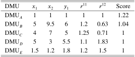
Using a numerical example with two inputs and one output presented in Table 1, we identify improvement targets for inefficient DMUs using the proposed approach. First, we solve model 2 and confirm that DMUs C, D, and E are DEA-R efficient. These three efficient DMUs are then used to construct the efficient frontier \(E_\text{R}\). The numerical example is illustrated in Fig. 1 in which the line segments CE and DE represent the efficient frontier \(E_\text{R}\). In this example, because only one output \(y_{1o}\) exists, the constraint corresponding to Eq. 6 is given as follows:
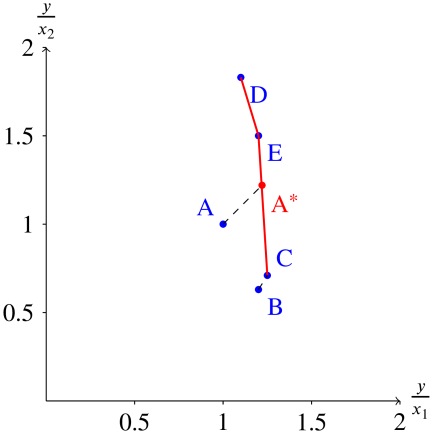
Fig. 1. Visualization of Table 1.
Table 2. Results for Table 1.
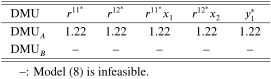
Table 3. Example with two inputs and two outputs.
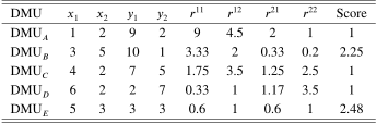
Table 4. Results for Table 3.

Table 5. Identified improvement targets: first iteration.
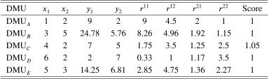
Table 6. Results for Table 5.

3.2.2. Example with Two Inputs and Two Outputs
Using a numerical example with two inputs and two outputs presented in Table 3, we again apply the proposed approach to identify improvement targets for inefficient DMUs. We begin by solving model 2, from which DMUs A, C, and D are observed to be DEA-R efficient. These three efficient DMUs are then used to construct the efficient frontier \(E_\text{R}\). Because this example involves two outputs, to identify the improvement targets using \(y_{2o}\) as the reference, the corresponding additional constraint is as follows:
Table 7. Identified improvement targets: second iteration.
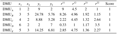
Nevertheless, selecting the maximum value can alter \(E_\text{R}\). Therefore, it is necessary not only to verify whether the inefficient DMU becomes efficient after converting the identified improvement targets into ratio indicators, but also to check whether the originally efficient DMUs remain efficient. Accordingly, the efficiency of each DMU is examined. As presented in Table 5, DMU\(_C\), which was originally efficient, becomes inefficient. Following the aforementioned procedure, the improvement target for the DMU\(_C\) can to be identified, and the results are presented in Table 6. Subsequently, the efficiency verification is conducted again, and the results are presented in Table 7. Because both improvement targets and originally efficient DMUs are efficient when converted into ratio indicators, the improvement target identification process is complete.
3.3. Implementation of the Proposed Approach
The proposed approach can be formalized as the following algorithm.
-
Step 1.
Solve model 2 to identify DEA-R efficient DMUs and construct the efficient frontier \(E_\text{R}\). Proceed to Step 2.
-
Step 2.
Use the efficient frontier \(E_\text{R}\) constructed in Step 1, select a reference output (\(y_{1o}\)) and two reference inputs (\(x_{\tilde mo}\) and \(x_{\bar mo}\)), and solve model 8 for each inefficient DMU. Obtain
\begin{align} \boldsymbol{r}^*&= \bigl(r^{{11}^*}, r^{{12}^*}, \dots , r^{{1m}^*},\nonumber\\ &\phantom{=~}~~~r^{{21}^*}, r^{{22}^*}, \dots ,r^{{2m}^*},\nonumber\\ &\phantom{=~}~~~\dots , \nonumber\\ &\phantom{=~}~~~r^{{s1}^*}, r^{{s2}^*}, \dots , r^{{sm}^*}\bigr)^\top, \end{align}to identify output-based improvement targets. Proceed to Step 3.
-
Step 3.
Classify into two cases based on whether model 8 has a feasible solution.
-
If a solution exists for each inefficient DMU, proceed to Step 4 to identify the corresponding improvement targets.
-
If no solution exists for DMU\(_k\), then a direct improvement target is assigned among the current efficient DMUs depending on the scenario. The improvement target for DMU\(_k\) without solutions have been identified. Proceed to Step 4 to identify improvement targets for the other DMUs with solutions.
-
-
Step 4.
For each inefficient DMU with a solution obtained in Step 3:
-
If there is one output (\(s = 1\)), the improvement target for \(y_{1o}\) is determined using
\begin{align} r^{{1\tilde{m}}^*} x_{\tilde{m}o} = r^{{1\bar{m}}^*} x_{\bar{m}o}. \end{align}The algorithm ends, and improvement targets have been identified for all inefficient DMUs.
-
If there are multiple outputs (\(s \geq 2\)): The selection of the reference output depends on the user or the scenario. Here, we identify the output improvement targets using a general method based on the following additional constraint (\(y_{1o}\) as the reference output).
\begin{align} r^{{1\tilde{m}}} x_{\tilde{m}o} = r^{{1\bar{m}}} x_{\bar{m}o}. \end{align}-
(1)
Use \(r^{{1\tilde{m}}^*}\) and \(r^{{1\bar{m}}^*}\) obtained in Step 2 to identify the improvement target for \(y_{1o}\), denoted as \(y_{1o}^*\). Because of the selection of \(y_{1o}\) as the reference, \(y_{1o}^* = r^{{1\tilde{m}}^*} x_{\tilde{m}o} = r^{{1\bar{m}}^*} x_{\bar{m}o}\).
-
(2)
Use \(r^{{2\tilde{m}}^*}\) and \(r^{{2\bar{m}}^*}\) obtained in Step 2 to identify the improvement target for \(y_{2o}\), denoted as \(y_{2o}^*\). If \(r^{{2\tilde{m}}^*} x_{\tilde{m}o} = r^{{2\bar{m}}^*} x_{\bar{m}o}\), it is accepted as the improvement target for \(y_{2o}\); otherwise, the larger value is selected as the improvement target for \(y_{2o}\). In other word, \(y_{2o}^* = \max\{r^{{2\tilde{m}}^*} x_{\tilde{m}o}, r^{{2\bar{m}}^*} x_{\bar{m}o}\}\).
-
(3)
This procedure is applied to other outputs as well, and the efficient frontier \(E_\text{R}\) may be changed and extended accordingly. Proceed to Step 5.
-
(1)
-
-
Step 5.
Verify whether the ratio indicators constructed using the identified improvement targets lie on \(E_\text{R}\).
-
If they do, the algorithm ends, and improvement targets have been identified for all inefficient DMUs.
-
If not, return to Step 1 and repeat the process for the corresponding DMUs.
-
Table 8. Summary of inputs and outputs for DMUs and targets.
4. Numerical Experiments
4.1. Dataset and Experimental Setup
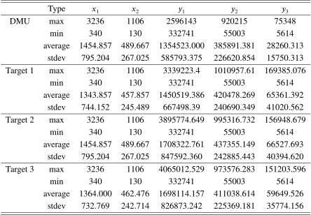
In this study, we employ the real-world dataset provided in 10 that was originally used for DEA-R analysis. The dataset consists of 21 hospitals characterized by two inputs and three outputs. The inputs are the numbers of beds and physicians, and the outputs are the numbers of outpatients, inpatients, and surgeries. The statistical summary of the dataset is presented in Table 8. Using the approach proposed in Section 3, we identify the improvement targets for the 21 hospitals by alternately selecting each of the three outputs as the reference output. Consequently, three types of improvement targets are identified for each hospital (hereafter referred to as a DMU). The statistical information on these improvement targets is also presented in Table 8. The differences among the three types of improvement targets, which arise from the selection of the reference output, are further examined later through density plots and sensitivity analysis.
Table 9. Details of the three computational procedures.
4.2. Improvement Targets Identified Using the Proposed Approach
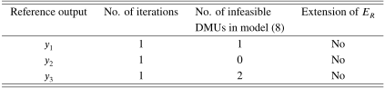
The proposed approach is then applied to the dataset, and the details of the three computational procedures, which alternately select three outputs to identify the improvement targets, are presented in Table 9. Although DMUs exist for which no feasible solution is obtained, no expansion of the feasible set \(E_\mathrm{R}\) is observed. Thus, irrespective of the output selected as the reference, the proposed approach is able to identify improvement targets for all inefficient DMUs within a single iteration.
In existing DEA-R models, improvement targets are typically provided only in the proportional form. Because a single input or output simultaneously contributes to multiple proportional indicators, converting these targets into non-proportional forms is inherently difficult. For instance, Gerami et al. 10 proposed ratio-based variants of the SBM model; however, their models did not provide concrete input and output improvement targets. Mozaffari et al. 8 proposed a central resource allocation model based on DEA-R to derive input and output improvement targets for inefficient DMUs. However, when these targets are converted into ratio indicators, they might become inefficient; this is inconsistent with the efficiency concept underlying DEA-R. Related studies by Mozaffari et al. 22,23 focused on identifying efficient surfaces and reference DMUs for benchmarking purposes but did not explicitly provide concrete input and output improvement targets. In contrast, the approach proposed in this study is capable of generating concrete (non-proportional) improvement targets for either inputs or outputs. Furthermore, their efficiency is guaranteed when these improvement targets are converted into ratio indicators.
Figure 2 presents density plots comparing the observed values and the corresponding improvement targets identified from the three computational procedures. These plots provide a visual comparison of both the deviations between the observed values and targets, and the differences among the three types of improvement targets. The distributions of the improvement targets are visually very similar across the three procedures, suggesting that the selection of the reference output has only a limited impact on the resulting improvement targets. This visual observation is further quantitatively examined using the sensitivity analyses described in Section 4.3.
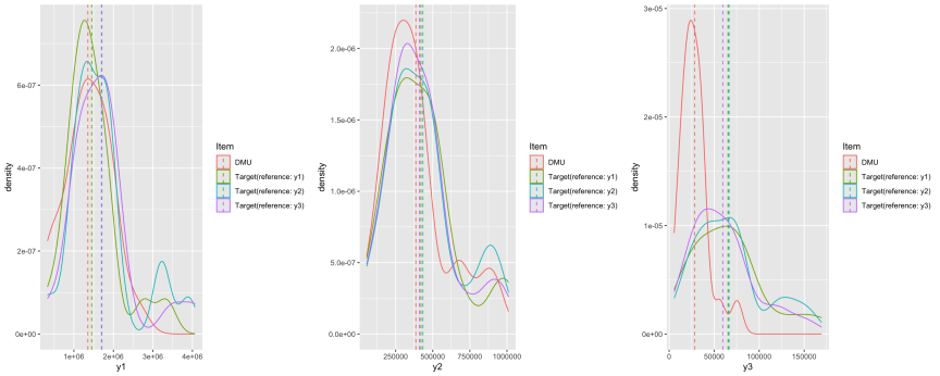
Fig. 2. Density plots for the identified improvement targets.
4.3. Sensitivity Analysis
To quantitatively assess the similarity among the improvement targets identified from the three computational procedures, we propose a new indicator called the target consistency index (TCI). Let \(t_j^{(k)}\) denote the improvement target for DMU\(_j\) identified from the \(k\)-th computational procedure \((k=1,2,3)\), and let \(d_j\) represent the observed input and output levels of DMU\(_j\). The TCI for DMU\(_j\) is defined as follows:
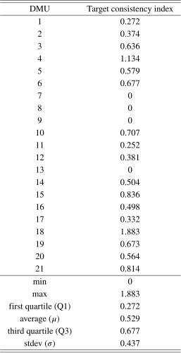
Table 10. Target consistency index for each DMU.
The numerator represents the average pairwise distance among the three improvement targets, and the denominator represents the average distance from the observed DMU to each improvement target. In this study, the absolute value is used as the distance measure. This selection is consistent with the objective function of model 8 used in our numerical experiment that minimizes the sum of slacks. Because the slack corresponds to absolute deviations from the efficient frontier, the absolute distance appropriately reflects the notion of distance embedded in the optimization model.
4.3.1. Interpretation of the Index
The TCI is designed to evaluate the relative dispersion of improvement targets across selecting the three different reference outputs.
-
A small value of \(\mathrm{TCI}_j\) indicates that the three improvement targets are close to one another relative to their distances from the original DMU, implying a high level of consistency.
-
A large value of \(\mathrm{TCI}_j\) indicates variation among the improvement targets.
-
\(\mathrm{TCI}_j = 0\) indicates that the DMU is efficient.
4.3.2. Numerical Results
Table 10 presents the TCI for all 21 DMUs. The minimum value is \(0\), the maximum value is \(1.883\), and the average value (\(\mu\)) is \(0.529\), with a standard deviation (\(\sigma\)) of \(0.437\). The first and third quartiles are \(0.272\) and \(0.677\), respectively, indicating that the majority of DMUs exhibit TCI values well below 1.403 (\(\mu + 2\sigma\)). The relatively large TCI values (\(1.883 > 1.403\)) observed for DMU\(_{18}\) can be explained by the discussion in Step 3 of the proposed approach in Section 3.3.(3) Owing to the structure of the dataset, the DMU\(_{18}\) corresponds to an irregular case in which no feasible solution is obtained, similar to DMU\(_B\) illustrated in Fig. 1. Consequently, a direct improvement target is assigned to DMU\(_{18}\) from the set of currently efficient DMUs, depending on the selected shortest-distance scenario. Although the improvement target is still identified based on the shortest-distance principle, both input and output adjustments are required for the irregular DMU\(_{18}\). As a result, its TCI values are relatively larger than those of the DMUs that involve only output adjustments according to the proposed approach.
Figure 3 illustrates the distribution of TCI values across the 21 DMUs. Overall, the results suggest that the improvement targets identified from the three computational procedures, each corresponding to a different selection of reference output, are highly consistent for most DMUs. Although the DMU\(_{18}\) exhibits relatively large TCI values, the overall distribution confirms that the differences among the three improvement targets are generally minor. Therefore, the numerical evidence supports the claim that the proposed approach yield largely similar improvement targets, despite differences in the selection of the reference output.
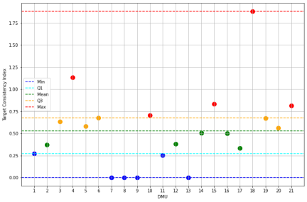
Fig. 3. Target consistency index distribution.
5. Conclusion and Future Research
In DEA-R, identifying concrete improvement targets is challenging because of the nature of ratio data. This study proposes an approach to identify valid improvement targets in the DEA-R framework. The proposed approach begins with the construction of the DEA-R efficient frontier and identifies output improvement targets while maintaining the input constant. Consequently, the identified targets are guaranteed to lie on the efficient frontier. Because the efficient frontier is explicitly constructed, various improvement targets can be specified depending on the decision-making scenario, thereby enhancing the practical applicability and flexibility of the approach.
The proposed approach searches for improvement targets within the constructed \(E_\text{R}\); however, \(E_\text{R}\) may be expanded and model 8 could sometimes be infeasible. Although we outlined certain countermeasures, these shortcomings must be addressed, and further extensions of the proposed approach are expected in the future. In addition, when multiple outputs are available, we verified through numerical experiments using real data that the selection of the reference output has limited influence on the resulting improvement targets. Based on this observation, the selection of input pairs is expected to have limited influence on the results; however, a rigorous verification remains an important topic for future research. Furthermore, among the various DEA models, slacks-based models are particularly popular because they allow for the simultaneous improvement of both inputs and outputs, rather than focusing on only one side. By contrast, the approach proposed in this study can only provide improvement targets for either the inputs or outputs, but not both simultaneously. Therefore, the development of a DEA-R approach that can offer simultaneous improvement targets for both inputs and outputs is a possible direction for future research. Moreover, the application of the proposed approach to case studies is expected in the future.
Acknowledgments
The authors gratefully acknowledge the anonymous editor and the two anonymous reviewers for their insightful comments and constructive suggestions that have significantly improved the quality of this paper. This work was supported by JSPS KAKENHI (Grant-in-Aid for Early-Career Scientists), Grant Number JP25K16715.
Footnotes
(1) This study focuses on situations in which input (\(x\)) and output (\(y\)) data are available in their original forms, rather than being inherently in the ratio form. In these cases, ratios such as \({y}/{x}\) and \({x}/{y}\) are constructed from the original inputs and outputs to evaluate the efficiency of DMUs. Therefore, the focus of this study differs from that of 2,3, which focus specifically on data expressed in the ratio form.
(2) \(\displaystyle r^{{21}^*}={25}/{13} \fallingdotseq 1.92, r^{{22}^*} ={15}/{13} \fallingdotseq 1.15.\) \(\displaystyle r^{{21}^*}x_{1B}=r^{{22}^*}x_{2B}= {25}/{13} \times 3 = {15}/{13} \times 5 = {75}/{13} \fallingdotseq 5.76.\)
(3) Although the TCI value of DMU\(_4\) (\(1.134 < 1.403\)) is below 1.403, it is still relatively large. That is because DMU\(_4\) shares a similar situation with DMU\(_{18}\). Owing to the structure of the dataset, both DMUs correspond to irregular cases in which no feasible solution can be obtained, as discussed in Step 3 of Section 3.3.
- [1] A. Charnes, W. W. Cooper, and E. Rhodes, “Measuring the efficiency of decision making units,” European J. of Operational Research, Vol.2, No.6, pp. 429-444, 1978. https://doi.org/10.1016/0377-2217(78)90138-8
- [2] O. B. Olesen, N. C. Petersen, and V. V. Podinovski, “Efficiency analysis with ratio measures,” European J. of Operational Research, Vol.245, No.2, pp. 446-462, 2015. https://doi.org/10.1016/j.ejor.2015.03.013
- [3] O. B. Olesen, N. C. Petersen, and V. V. Podinovski, “Efficiency measures and computational approaches for data envelopment analysis models with ratio inputs and outputs,” European J. of Operational Research, Vol.261, No.2, pp. 640-655, 2017. https://doi.org/10.1016/j.ejor.2017.02.021
- [4] O. Despić, M. Despić, and J. C. Paradi, “DEA-R: Ratio-based comparative efficiency model, its mathematical relation to DEA and its use in applications,” J. of Productivity Analysis, Vol.28, No.1, pp. 33-44, 2007. https://doi.org/10.1007/s11123-007-0050-x
- [5] C.-K. Wei, L.-C. Chen, R.-K. Li, and C.-H. Tsai, “Using the DEA-R model in the hospital industry to study the pseudo-inefficiency problem,” Expert Systems with Applications, Vol.38, No.3, pp. 2172-2176, 2011. https://doi.org/10.1016/j.eswa.2010.08.003
- [6] C.-K. Wei, L.-C. Chen, R.-K. Li, and C.-H. Tsai, “A study of developing an input-oriented ratio-based comparative efficiency model,” Expert Systems with Applications, Vol.38, No.3, pp. 2473-2477, 2011. https://doi.org/10.1016/j.eswa.2010.08.036
- [7] C.-K. Wei, L.-C. Chen, R.-K. Li, and C.-H. Tsai, “Exploration of efficiency underestimation of CCR model: Based on medical sectors with DEA-R model,” Expert Systems with Applications, Vol.38, No.4, pp. 3155-3160, 2011. https://doi.org/10.1016/j.eswa.2010.08.108
- [8] M. R. Mozaffari, J. Gerami, and J. Jablonsky, “Relationship between DEA models without explicit inputs and DEA-R models,” Central European J. of Operations Research, Vol.22, pp. 1-12, 2014. https://doi.org/10.1007/s10100-012-0273-4
- [9] R. D. Banker, A. Charnes, and W. W. Cooper, “Some models for estimating technical and scale inefficiencies in data envelopment analysis,” Management Science, Vol.30, No.9, pp. 1078-1092, 1984. https://www.jstor.org/stable/2631725
- [10] J. Gerami, M. R. Mozaffari, P. F. Wanke, and H. Correa, “A novel slacks-based model for efficiency and super-efficiency in DEA-R,” Operational Research, Vol.22, pp. 3373-3410, 2022. https://doi.org/10.1007/s12351-021-00679-6
- [11] X. Wang, H. Iwamoto, and T. Hasuike, “A slacks-based DEA-R approach with an application to Japanese banks,” J. Adv. Comput. Intell. Intell. Inform., Vol.30, No.1, pp. 67-77, 2026. https://doi.org/10.20965/jaciii.2026.p0067
- [12] M. Soltanifar, M. Ghiyasi, and H. Sharafi, “Inverse DEA-R models for merger analysis with negative data,” IMA J. of Management Mathematics, Vol.34, No.3, pp. 491-510, 2023. https://doi.org/10.1093/imaman/dpac001
- [13] J. Gerami, M. R. Mozaffari, and P. F. Wanke, “A multi-criteria ratio-based approach for two-stage data envelopment analysis,” Expert Systems with Applications, Vol.158, Article No.113508, 2020. https://doi.org/10.1016/j.eswa.2020.113508
- [14] P. Kamyab, M. R. Mozaffari, J. Gerami, and P. F. Wankei, “Two-stage incentives system for commercial banks based on centralized resource allocation model in DEA-R,” Int. J. of Productivity and Performance Management, Vol.70, No.2, pp. 427-458, 2021. https://doi.org/10.1108/IJPPM-11-2018-0396
- [15] D. Akbarian, “Network DEA based on DEA-ratio,” Financial Innovation, Vol.7, No.1, Article No.73, 2021. https://doi.org/10.1186/s40854-021-00278-6
- [16] J. Gerami, R. Kiani Mavi, R. Farzipoor Saen, and N. Kiani Mavi, “A novel network DEA-R model for evaluating hospital services supply chain performance,” Annals of Operations Research, Vol.324, pp. 1041-1066, 2023. https://doi.org/10.1007/s10479-020-03755-w
- [17] W. W. Cooper, K. S. Park, and J. T. Pastor, “RAM: A range adjusted measure of inefficiency for use with additive models, and relations to other models and measures in DEA,” J. of Productivity Analysis, Vol.11, No.1, pp. 5-42, 1999. https://doi.org/10.1023/A:1007701304281
- [18] K. Tone, “A slacks-based measure of efficiency in data envelopment analysis,” European J. of Operational Research, Vol.130, No.3, pp. 498-509, 2001. https://doi.org/10.1016/S0377-2217(99)00407-5
- [19] Q. An, Q. Wu, X. Zhou, and X. Chen, “Closest target setting for two-stage network system: An application to the commercial banks in China,” Expert Systems with Applications, Vol.175, Article No.114799, 2021. https://doi.org/10.1016/j.eswa.2021.114799
- [20] Q. Zhu, J. Aparicio, F. Li, J. Wu, and G. Kou, “Determining closest targets on the extended facet production possibility set in data envelopment analysis: Modeling and computational aspects,” European J. of Operational Research, Vol.296, No.3, pp. 927-939, 2022. https://doi.org/10.1016/j.ejor.2021.04.019
- [21] C. Kao, “Closest targets in the slacks-based measure of efficiency for production units with multi-period data,” European J. of Operational Research, Vol.297, No.3, pp. 1042-1054, 2022. https://doi.org/10.1016/j.ejor.2021.05.050
- [22] M. R. Mozaffari, F. Dadkhah, J. Jablonsky, and P. F. Wanke, “Finding efficient surfaces in DEA-R models,” Applied Mathematics and Computation, Vol.386, Article No.125497, 2020. https://doi.org/10.1016/j.amc.2020.125497
- [23] M. Mozaffari, J. Gerami, P. Wanke, P. Kamyab, and M. Peyvas, “Ratio-based data envelopment analysis: an interactive approach to identify benchmark,” Results in Control and Optimization, Vol.6, Article No.100081, 2022. https://doi.org/10.1016/j.rico.2021.100081
- [24] X. Wang, K. Lu, J. Shi, and T. Hasuike, “A new mip approach on the least distance problem in DEA,” Asia-Pacific J. of Operational Research, Vol.37, No.6, Article No.2050027, 2020. https://doi.org/10.1142/S021759592050027X
- [25] M. Kameli, B. Daneshian, F. M. Khiyabani, and F. H. Lotfi, “Target setting and benchmarking by the possibility of selecting the closest alternative benchmark,” RAIRO-Operations Research, Vol.59, No.1, pp. 101-114, 2025. https://doi.org/10.1051/ro/2024130
This article is published under a Creative Commons Attribution-NoDerivatives 4.0 Internationa License.