
Research Paper:
Intelligent Prediction of the Hearth Lining Temperature in Blast Furnaces Based on Spatiotemporal Feature Fusion
Qifu Chen*1,*2, Jiaxin Cheng*3,*4, Jianqi An*1,*3,*4,†
 , and Jinhua She*5
*1School of Future Technology, China University of Geosciences
No.388 Lumo Road, Wuhan, Hubei 430074, China
*2Hunan Valin Lianyuan Iron and Steel Co., Ltd.
No.1005 Jinxing North Road, Louxing District, Loudi, Hunan 417009, China
*3School of Artificial Intelligence and Automation, China University of Geosciences
No.388 Lumo Road, Wuhan, Hubei 430074, China
*4Hubei Key Laboratory of Advanced Control and Intelligent Automation for Complex Systems
No.388 Lumo Road, Wuhan, Hubei 430074, China
*5School of Engineering, Tokyo University of Technology
1404-1 Katakura machi, Hachioji, Tokyo 192-0982, Japan
†Corresponding author

Accurate forecasting of the hearth lining temperature in blast furnaces is essential for operational safety and efficiency, however it remains challenging owing to the complex spatiotemporal coupling and time-lag effects among process variables. To address this issue, we present a new spatiotemporal feature modeling framework that integrates gated recurrent units (GRUs) with a dual-attention mechanism to capture multi-scale temporal dependencies and dynamically assess variable importance. A convolutional neural network module is incorporated to extract localized spatial features from the time-series data, thereby enhancing the representation of the underlying metallurgical mechanisms. The validation on real industrial data showed that the proposed model achieved a root mean square error of 0.0523 and a hit rate of 94.26%, outperforming conventional long short-term memory and GRU models. This approach offers a reliable solution for intelligent health monitoring and proactive maintenance in modern data-driven ironmaking operations under highly dynamic and uncertain conditions.
1. Introduction
The iron and steel industry is a fundamental pillar of modern manufacturing. Ironmaking in blast furnaces (BFs) remains the dominant route for large-scale hot metal production. Among the various operating parameters, the hearth lining temperature is a key indicator for evaluating the furnace integrity, residual lining thickness, and long-term campaign safety. Abnormal heating or accelerated erosion may trigger severe incidents such as hearth breakout, posing substantial risks to equipment and personnel 1. Therefore, developing accurate and reliable methods for predicting the hearth lining temperature is of great significance for the intelligent monitoring of BFs and proper operational decision-making.
However, this task remains highly challenging because of the inherent complexity of the BF process. The evolution of the hearth lining temperature is governed by multi-scale physicochemical reactions and intricate interactions among burden descent, gas–solid flow, and heat transfer mechanisms 2. These interactions produce heterogeneous time delays in which different process variables exert their influence over distinct temporal horizons, ranging from one to two hours for cooling-related parameters to two through four hours for gas flow and combustion conditions. Moreover, the process exhibits strong spatiotemporal coupling because local fluctuations propagate across the furnace zones and interact dynamically with other variables. These properties result in a substantially nonlinear, time-varying behavior that is difficult to describe analytically or capture using conventional modeling techniques.
Methods for predicting the BF parameters are broadly classified into mechanism-based and data-driven approaches 3. Mechanism-based modeling relies on mathematical descriptions of underlying physicochemical processes. For example, the gas flow distribution was predicted to assess the internal furnace conditions 4, and the chaotic analysis was applied to characterize the carbon monoxide utilization rate 5. Additionally, an inverse estimation of the internal temperature profiles, and thus the gas distribution, was realized using boundary measurements 6. These mechanism-driven models provide a valuable foundation for an in-depth analysis of BF operational states by integrating domain knowledge of the ironmaking process in BFs. However, most rely on idealized assumptions that may limit their accuracy and generalizability in complex industrial environments.
Data-driven modeling methods, based on one or more data models and historical data, have been used to predict the hearth lining temperature in combination with the actual characteristics of industrial production 7. In recent years, data-driven methods have been widely applied to analyze BF production processes. For example, Lu et al. 8 integrated real-time wavelet filtering into machine learning to predict combustion zone temperature. Su et al. 9 improved the multilayer extreme learning machine using an adaptive particle swarm optimization algorithm and an ensemble model for temperature prediction. Jiao et al. 10 proposed a collaborative multiple rank regression method to predict temperature based on acquired images and physical variables. Chen et al. 11 developed a dynamic mechanism module to comprehensively characterize the input–output dynamic relationships, while integrating real-time data from an infrared vision-based molten iron temperature detection system into the model for quality variable prediction, thereby improving the prediction performance.
Machine learning methods have emerged as powerful approaches for BF parameter prediction by leveraging historical data to identify complex non-linear patterns 12. Early research in this field primarily relied on shallow models, such as support vector machines 13 and \(k\)-nearest neighbors 14. In recent years, deep learning techniques, particularly recurrent neural networks, such as long short-term memory (LSTM) 15 and gated recurrent unit (GRU), have gained prominence owing to their superior capability in modeling temporal dependencies in process data 16. Representative applications include the artificial neural network—a nonlinear autoregressive exogenous model proposed by Bozkurt et al. 17 that predicts the hot metal temperature to support operational decision-making, and the generalized regression neural network—a particle swarm optimization model developed by Guo et al. 18 that improved the prediction accuracy of furnace status variables through intelligent parameter optimization.
Although published approaches have improved our modeling capabilities, critical gaps remain in the accurate prediction of the hearth lining temperature in BFs. Although mechanism-based models are constrained by idealized assumptions, mainstream data-driven approaches, including conventional recurrent neural networks, face three interrelated challenges. First, their inherent black-box nature often decouples them from underlying metallurgical mechanisms, limiting their interpretability and operational reliability. Second, these models cannot typically explicitly address the non-uniform time delays inherent among the different process variables. Third, the local spatial correlations within multivariate time series are widely overlooked; this represents a significant oversimplification of the process dynamics. Collectively, these limitations restrict the accuracy and generalizability of models in complex industrial environments.
To address these challenges, this paper presents a new spatiotemporal feature integration modeling framework for predicting the hearth lining temperature. The main contributions of this study are summarized as follows:
-
(1)
A unified spatiotemporal prediction architecture was developed by integrating a GRU, feature-dimension dual-attention mechanism, and convolutional neural network (CNN), enabling the joint modeling of long-term temporal dependencies and local spatial correlations.
-
(2)
A feature-dimension attention module was designed to dynamically quantify variable-specific influence intensities, allowing the model to effectively learn and compensate for heterogeneous time delays.
-
(3)
A CNN-based spatial perception component was introduced to capture the local structural patterns among multivariate process variables, improving feature alignment and enhancing physical interpretability.
The remainder of this paper is organized as follows. Section 2 presents the BF ironmaking mechanism and overall methodological framework. Section 3 describes the proposed spatiotemporal modeling approach. Section 4 presents an experimental analysis and comparative evaluation. Finally, Section 5 concludes the study and outlines future research directions.
2. Problem Formulation and Methodological Framework
This section describes the proposed integrated spatiotemporal model. It begins with a formal definition of the prediction problem, followed by a systematic exposition of the two core components: the multi-scale temporal feature extraction and local spatial feature perception modules. This section concludes by presenting the complete integrated framework.
2.1. Spatiotemporal Characteristics of the BF Ironmaking Process
A BF is a large-scale countercurrent reactor with intensive heat and mass transfer. Its internal conditions evolve through coupled physicochemical reactions occurring in multiple zones, including the lump, cohesive, dripping, raceway, and hearths. Among these zones, the hearth plays a critical role because its thermal state directly determines the residual lining thickness and campaign safety 19. Therefore, understanding the spatiotemporal evolution of the hearth lining temperature is essential for establishing an effective prediction model.
From a modeling perspective, two fundamental characteristics make the prediction problem extremely challenging:
-
(1)
The operational parameters affect the lining temperature with distinct lags. Changes in the gas flow and thermal load appear after 2–4 hours, while cooling adjustments respond within 1–2 hours. These uneven delays require models that can represent variable temporal dependencies.
-
(2)
BF variables interact rather than acting independently. Local changes in the blast temperature, pressure, or permeability propagate and couple with other factors, generating complex spatial correlations and structures in multivariate time series that extend beyond point-wise temporal models.
Conventional data-driven models often fail to simultaneously capture these temporal and spatial complexities, resulting in inaccurate predictions and limited operational utility. BFs are complex reactors involving a series of chemical and physical reactions. Inside a BF, iron ore and other iron-containing compounds undergo redox reactions with coke at high temperatures and pressures to produce molten iron and BF gas 20. Fig. 1 illustrates the BF ironmaking process.
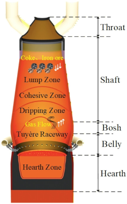
Fig. 1. BF ironmaking process.
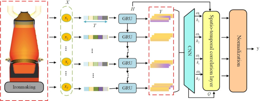
Fig. 2. Schematic of the multi-dimensional spatiotemporal correlated feature fusion model for quality variable prediction.
2.2. Integrated Spatiotemporal Modeling Framework
To address the aforementioned challenges, we propose an integrated spatiotemporal modeling framework designed for accurately forecasting the BF hearth lining temperature. The core idea is to model multi-scale temporal dependencies and inter-variable spatial correlations using a specialized neural network.
The overall structure of the proposed model is shown in Fig. 2. It comprises two synergistic components:
-
(1)
Temporal feature extraction using the GRU. GRU networks were employed to capture long-term temporal dependencies and cumulative process effects while avoiding vanishing gradients. They provide a compact representation of historical evolution by generating hidden states for multivariate inputs.
-
(2)
Feature-dimensional attention for non-uniform delay modeling. A feature-dimensional attention mechanism is introduced to dynamically evaluate the relevance of each variable at each time step. This component enables the model to automatically learn variable-specific influence intensities and effectively approximate heterogeneous delay vectors.
-
(3)
CNN-based local spatial feature perception. To capture the spatial correlations among variables within a short time span, a CNN module was applied to the GRU-generated hidden state matrix. This operation recognizes localized structural patterns, such as rising trends, coordinated fluctuations, and segmental correlations, which reflect the underlying metallurgical interactions.
Together, these modules form an integrated spatiotemporal architecture that transforms raw BF operational data into a physically meaningful and highly predictive representation of the hearth lining temperature.
3. Modeling and Analysis of Spatiotemporal Characteristics
In this section, we describe the proposed spatiotemporal model. It formally defines the prediction problem, introduces multi-scale temporal feature extraction and local spatial feature perception modules, and concludes with an integrated framework.
3.1. Problem Formulation and Modeling Rationale
Accurate prediction of the hearth lining temperature in the BF requires the formalization of the complex spatiotemporal relationships between process variables and the target quality variable 21. The problem is defined as follows: given \(N\) process variables, each forming a time series of length \(M\), the objective is to predict the future value of quality variable \(y_t\) (hearth lining temperature) at time \(t\).
Conventional approaches often rely on simplified temporal assumptions. The most basic form is the synchronous model that assumes all variables exert an instantaneous influence at time \(t\).
A common refinement is the uniform-lag model that introduces a single time delay \(\tau\) for all variables
Although these formulations provide tractable baselines, they fundamentally misrepresent the BF ironmaking process. The synchronous model ignores temporal causality, whereas the uniform-lag model fails to capture the empirically observed variable-specific delay times that range from one to four hours for different parameters.
A more realistic approach involves modeling a distinct time delay \(\tau_{i}\) for each variable \(i\), defined by a delay vector
This formulation accounts for non-uniform delays. However, it remains limited by focusing on a single discrete historical time step for each variable, thereby neglecting the cumulative effects of the entire recent history of each variable and the dynamic interactions between variables. To overcome these limitations, a comprehensive spatiotemporal feature representation is proposed. This representation integrates the cumulative influence of all variables over a historical window of length \(L\), weighted by their dynamically computed importance
3.2. Temporal Feature Extraction Using GRU and Feature Attention
The extended smelting cycle of a BF necessitates modeling the continuous cumulative effects of the process variables over time. Conventional approaches struggle to handle the non-uniform time delays inherent in the process, in which different parameters affect the target quality variable over varying lag times 22. To address this issue, a multi-scale temporal feature extraction network is presented, integrating GRU with a feature-dimension attention mechanism.
The GRU architecture serves as the foundational temporal modeling component, selected for its efficacy in capturing long-range dependencies while mitigating the vanishing gradient problem 23. Compared with the LSTM network, the GRU adopts a more streamlined gating mechanism that often results in faster convergence and comparable performance on industrial-scale datasets. This capability to learn complex temporal patterns is further enhanced by a feature-dimension attention mechanism that explicitly addresses the challenge of non-uniform variable influence.
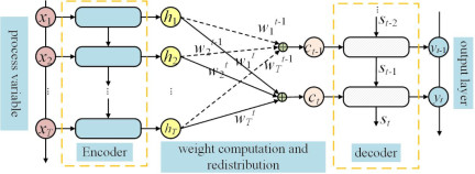
Fig. 3. Schematic of the attention weight extraction mechanism.
As illustrated in Fig. 3, the attention component dynamically recalibrates the importance of each process variable at every time step by performing soft-feature weighting based on its instantaneous relevance to the prediction target. Together, this integrated design enables the model to model the evolution of process states and adaptively focus on the most pertinent variables from the high-dimensional input space, directly addressing the core challenges of dynamic coupling and variable-specific time delays.
The overall architecture of the proposed temporal feature extraction model is shown in Fig. 4. The input is a multivariate time series \(X = [x_{1}, x_{2}, \dots, x_{T}]\), where \(x_{t} = (x_{t}^{1}, x_{t}^{2}, \dots, x_{t}^{n}) \in \mathbb{R}^{n}\) denotes the values of \(n\) process variables at time \(t\). The model processes this input through three coordinated stages to generate a dynamically weighted temporal representation.
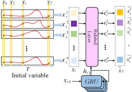
Fig. 4. Architecture of the proposed temporal feature extraction model.
The process begins with the input sequence being encoded by a GRU network that captures the fundamental temporal dependencies and produces a sequence of hidden states \(H = [h_{1}, h_{2}, \dots, h_{T}]\). Each hidden state \(h_t\) is updated based on current input \(x_t\) and previous hidden state \(h_{t-1}\), following the gating mechanisms defined in Eqs. 5–8.
Here \(r_t\) and \(z_t\) denote the reset and update gate, respectively; \(h'_{t}\) denotes the candidate hidden state; \(W_r\), \(W_z\), and \(W_h\) denote learnable weight matrices; \(\odot\) denotes the element-wise multiplication.
A feature-dimension attention layer is applied at each time step to dynamically quantify the influence of each variable 24. This layer evaluates the relevance of current input \(x_t\) to previous context \(h_{t-1}\) by computing an unnormalized attention score
The original input vector \(x_t\) is modulated by these weights to form a refined input vector
3.3. CNN-Based Local Spatial Feature Perception
Although the temporal model, as described in Section 3.2, effectively captures dynamic dependencies and non-uniform delays, it primarily operates on pointwise interactions between current input \(\tilde{x}_t\) and historical context \(h_{t-1}\). This approach computes feature weights based on the similarity between discrete points and may overlook richer local spatial patterns (for example, sequential shapes and structural trends) that exist among multiple variables over short time windows. Ignoring these inter-variable correlations can lead to feature mismatches during training, thereby limiting the prediction accuracy and model interpretability.
3.3.1. Motivation for Local Spatial Feature Optimization
Process variables temporally affect the quality variable and exhibit local spatial characteristics that reflect mechanistic interactions across different furnace zones 25. These local patterns are critical to accurately represent the underlying process dynamics and ensure robust feature learning.
In this study, the term “spatial” refers to the feature space rather than the physical geometric zones of the BF. Specifically, it denotes the structural correlations and proportional relationships between the different process variables in the input matrix. Although conventional correlation coefficients capture global linear relationships, they often fail to recognize local structural patterns (such as synchronized fluctuations across multiple sensors) within short time windows. The CNN module addresses this by leveraging its sliding window mechanism to capture the local “shapes” in the feature matrix.
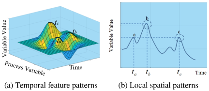
Fig. 5. Architecture of the spatiotemporal feature extraction model.
As shown in Fig. 5(a), we consider three feature points (a, b, and c) within a multivariate time window that exhibit similar proportional relationships. A point-wise similarity method (as described in Section 3.1) evaluates the matches between (a, b), (a, c), and (b, c) with equal probabilistic considerations. However, as illustrated in Fig. 5(b), points b and c share higher similarity in terms of local trend structure and contextual causality, making them the more meaningful match from a process perspective. Therefore, relying solely on point-wise attention can introduce mismatches that accumulate during training, leading to distorted feature representations and reduced prediction accuracy.
To address this issue, CNNs are introduced for local spatial feature perception. CNNs are well-suited for this task because of their sliding kernel mechanism that provides inherent translation invariance and enables robust pattern recognition within local receptive fields. By capturing inter-variable structures over short sequences, CNNs complement the temporal modeling capabilities of GRU and attention mechanisms, resulting in a more holistic spatiotemporal feature representation.
3.3.2. CNN-Based Local Spatial Feature Perception Model
The CNN module is applied to hidden state matrix \(H = [h_{1}, h_{2}, \dots, h_{T}]\) that is output by the GRU network, where each \(h_{t} \in \mathbb{R}^{d}\). To preserve the sequence boundaries, the matrix is padded appropriately, forming an expanded matrix \(Y \in \mathbb{R}^{d \times (T+l-1)}\), where \(l\) denotes the convolutional kernel size.
Let \(W^{k} \in \mathbb{R}^{m \times d \times l}\) and \(W^{q} \in \mathbb{R}^{m \times d \times l}\) denote the learnable kernel parameters for the key and query mappings, respectively, where \(m\) denotes the number of filters. The convolutional operation for the key matrix at position \(i\) is computed as follows:
Subsequently, key vector \(K_i\) is obtained by
Then, query vector \(Q \in \mathbb{R}^m\) is then given by
The complete architecture that integrates the proposed CNN-based spatial perception module with a temporal feature extraction network is shown in Fig. 6. This integrated design enhances feature alignment, reduces mismatches, and improves the overall robustness and accuracy of hearth lining temperature prediction.
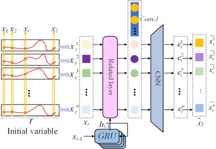
Fig. 6. Schematic of the feature extraction model structure after local spatial information perception optimization.
4. Experimental Analysis with Industrial Data
This section presents the evaluation of the effectiveness of the proposed integrated spatiotemporal model using real operational data from an industrial BF. This section details include dataset description, preprocessing, evaluation methodology, verification of the attention mechanism, ablation analysis of spatiotemporal components, comparative performance assessment against baseline models, and a discussion of practical implications for online process monitoring and control.
4.1. Data Preprocessing and Input Variable Selection
A BF is an ultra-large nonlinear integrated reactor, and its hearth lining temperature is influenced by numerous parameters. Based on the process mechanism analysis, as described in Section 2.2, and expert experience, the following parameters affecting the lining temperature were identified across the ironmaking timeline: raw material input properties, operational parameters during smelting, and output hot metal characteristics.
The experimental dataset was collected from a large-scale industrial BF over two days (May 15–16, 2023), yielding 12,000 valid samples. Although the time span was relatively short, the sampling frequency was high, and the furnace was operated under stable and representative working conditions, ensuring that the dataset effectively captured the thermal and operational dynamics relevant to the hearth lining temperature prediction. Similar short-range high-resolution datasets have been widely used in BF-related temperature forecasting studies.
Table 1. Selection of feature variables.
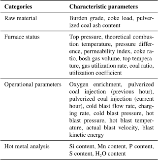
Considering the data quality and integrity, 28 parameters across the four categories were initially selected as characteristic inputs, as summarized in Table 1. Given the strong nonlinearity and coupling in BF processes, the maximal information coefficient (MIC) was employed instead of the Pearson correlation coefficient to evaluate both the linear and nonlinear relationships between the candidate variables and the target temperature. The MIC is calculated as follows:
The preprocessed dataset comprised 12,000 samples collected from a steel plant between May 15 and 16, 2023. It was split into training (9,000 samples) and test sets (3,000 samples) at a ratio of \(3:1\), with an additional validation set (1,500 samples) extracted from the training set to monitor the model training and prevent overfitting. To ensure data quality, the raw dataset was rigorously preprocessed. Outliers caused by sensor malfunctions were identified and removed using the \(3\sigma\) rule, and missing values were filled via linear interpolation. For variable selection, the MIC threshold was set to 0.3; variables with MIC values below this threshold were considered weakly correlated and excluded from the input set.
Although the dataset spanned a relatively short period (two days), the high sampling frequency yielded 12,000 samples that was sufficient for training the deep learning model to convergence. The selected period represents a stable operation, making it suitable for validating the proposed methodology, although long-term seasonal trends remain a subject for future studies.
4.2. Verification of the Attention Mechanism
The standard LSTM algorithm was selected as the baseline to validate the effectiveness of the proposed attention mechanism. Comparative experiments were conducted between the standard LSTM and an enhanced variant, namely feature attention-LSTM (FLSTM) that integrated the feature-dimension attention mechanism proposed in this study.
Figure 7 illustrates the features of the weight distribution enhanced by the attention mechanism. Notably, the contribution weights of different features at the same time step are adaptively adjusted during the training process. When combined with temporal attention, the model further dynamically modified the influence weights of different time steps for the same feature, thereby effectively achieving nonlinear time-delay adaptation within the sequence window. Notably, this learned distribution aligns well with the metallurgical time lags discussed in the Introduction section. As observed in Fig. 7, variables related to gas flow (for example, Sensor id: 4) exhibited higher attention weights at earlier time steps in the history window (reflecting a lag of \(>\) 2 h), whereas cooling-related variables (for example, Sensor id: 6) showed a peak influence at more recent time steps. This correspondence confirmed that the model successfully captured the underlying physical characteristics of the BF process.
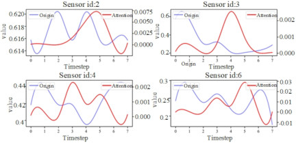
Fig. 7. Schematic of attention weight enhancement for different features and time steps (visualization of the last eight steps).
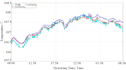
Fig. 8. Comparison of prediction results between LSTM and FLSTM models.
The prediction results on the test set are presented in Fig. 8. The cyan curve represents the actual hearth lining temperature, blue solid line denotes the prediction results of the standard LSTM, and red solid line indicates the prediction results of the FLSTM model. The model performance was evaluated using two metrics, hit rate (HR) and root mean square error (RMSE), that are defined as follows:
Thresholds \(\delta\) were selected based on the industrial operational standards. A threshold of 0.1 corresponds to a 10% relative error that is acceptable for general trend monitoring, whereas 0.01 represents a stricter 1% precision required for high-risk safety alerts.
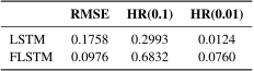
As summarized in Table 2, the FLSTM model significantly outperformed the standard LSTM, with RMSE reduced from 0.1758 to 0.0976 and the HR(0.1) increased from 29.93% to 68.32%. This demonstrated that the attention mechanism markedly enhanced the ability of the model to track the hearth lining temperature and improved the prediction accuracy.
Table 2. Performance comparison before and after integrating the attention mechanism.
4.3. Functional Verification of the Integrated Spatiotemporal Prediction Model
An experimental approach to hearth lining temperature prediction was conducted based on the full spatiotemporal feature fusion method described in this subsection. Consistent with the previous experiment, the dataset was split into training (9,000 samples) and test sets (3,000 samples), with a validation set (1,500 samples) extracted from the training set to optimize the hyperparameters.
During model training, the input sequence length and convolutional kernel size were identified as the key hyperparameters. Considering the model depth, potential overfitting risks, and relatively short time lag of lining temperature responses to internal reactions, the input sequence length was set to 15 based on the maximum process lag (approximately 4 h) observed in the domain knowledge. A sensitivity analysis via grid search indicated that a kernel size of 3 offered the best trade-off between feature extraction capability and computational efficiency. Regarding the computational cost, the average inference time of the proposed feature-time attention (FTA) model was approximately 15 ms per sample on a standard workstation. This speed is significantly faster than the data acquisition interval of the BF SCADA system, confirming the model’s feasibility for real-time online deployment.
The integrated model (denoted as FTA) dynamically predicts hearth lining temperature through a sequential multi-step process: it first uses GRU units to extract hidden state information from feature sequences, then applies a feature-dimension attention mechanism to weight variables according to their similarity to historical states, subsequently employs a CNN module to capture deep local spatial patterns from the hidden state matrix, and finally utilizes a self-attention mechanism to fuse the extracted spatiotemporal features before inputting them into the output layer to compute the final prediction of the hearth lining temperature.
Traditional shallow machine learning models, such as SVR or ELM, were not included in this comparison. Because the hearth lining temperature is governed by cumulative physicochemical reactions with distinct time lags, deep recurrent architectures (such as LSTM and GRU) are theoretically superior to static models in capturing these temporal dependencies.
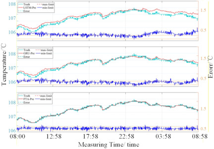
Fig. 9. Comparison chart of furnace lining temperature prediction results for each model.
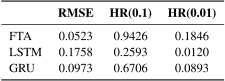
For performance validation, the proposed FTA model was compared with standard LSTM and GRU models. The prediction curves and actual values are shown in Fig. 9, and the performance metrics are compared in Table 3. The FTA model achieved a superior RMSE of 0.0523 and an HR(0.1) of 94.26%, significantly outperforming the LSTM (RMSE: 0.1758, HR(0.1): 25.93%) and GRU (RMSE: 0.0973, HR(0.1): 67.06%) benchmarks.
Table 3. Performance comparison of different prediction models.
The prediction of the BF hearth lining temperature was constrained by the diversity of the operational conditions and the complexity of the state parameters, exhibiting strong nonlinear and time-varying characteristics. This attention mechanism effectively addressed variable-specific time delays by continuously updating and quantifying the influence of each variable at different time steps. Furthermore, the CNN module enhanced the perception of local spatial patterns among variables, thereby reducing feature mismatches. These results confirmed that the constructed hearth lining temperature prediction model was effective and that the proposed spatiotemporal feature extraction framework achieves significantly higher accuracy than conventional models within the specified error range.
5. Conclusion
This study presented a unified spatiotemporal modeling framework to accurately predict the BF hearth lining temperature. The proposed architecture integrated GRU-based temporal modeling, a feature-dimension attention mechanism, and CNN-based spatial perception module to jointly capture heterogeneous time delays and local inter-variable structural patterns inherent in BF operations.
The feature-dimension attention mechanism enabled the model to learn variable-specific temporal influence and effectively compensated for non-uniform delays. The CNN module further enhanced feature alignment by extracting localized structural correlations among multivariate time series. Comprehensive validation using real industrial data demonstrated the superiority of the proposed approach. The model achieved an RMSE of 0.0523 and an HR(0.1) of 94.26%, significantly outperforming the standard LSTM and GRU baselines.
Future research should investigate hybrid modeling approaches that integrate data-driven learning with mechanistic knowledge, such as thermal balance and chemical reaction model that may further improve interpretability and generalization. Multitask learning frameworks for the simultaneous prediction of key thermal and quality indicators (for example, silicon content and gas utilization rate) should also be explored. Finally, developing online learning and adaptive update mechanisms is essential for maintaining long-term accuracy under evolving operational conditions.
Acknowledgments
This work was supported in part by the National Natural Science Foundation of China (NSFC) under Grant 62373336 and the 111 Project, China, under Grant B17040.
- [1] J. An, X. Shen, M. Wu, and J. She, “A multi-time-scale fusion prediction model for the gas utilization rate in a blast furnace,” Control Engineering Practice, Vol.92, Article No.104120, 2019. https://doi.org/10.1016/j.conengprac.2019.104120
- [2] C. Liu, J. Tan, J. Li, Y. Li, and H. Wang, “Temporal hypergraph attention network for silicon content prediction in blast furnace,” IEEE Trans. on Instrumentation and Measurement, Vol.71, Article No.2521413, 2022. https://doi.org/10.1109/TIM.2022.3219475
- [3] J. Chen, “A predictive system for blast furnaces by integrating a neural network with qualitative analysis,” Engineering Applications of Artificial Intelligence, Vol.14, No.1, pp. 77-85, 2001. https://doi.org/10.1016/S0952-1976(00)00062-2
- [4] J. Wei and X. Chen, “Blast furnace gas flow strength prediction using FMCW radar,” ISIJ Int., Vol.55, No.3, pp. 600-604, 2015. https://doi.org/10.2355/isijinternational.55.600
- [5] D. Xiao, J. An, Y. He, and M. Wu, “The chaotic characteristic of the carbon-monoxide utilization ratio in the blast furnace,” ISA Trans., Vol.68, pp. 109-115, 2017. https://doi.org/10.1016/j.isatra.2017.03.004
- [6] Y. Li, S. Zhang, Y. Yin, W. Xiao, and J. Zhang, “A novel online sequential extreme learning machine for gas utilization ratio prediction in blast furnaces,” Sensors, Vol.17, No.8, Article No.1847, 2017. https://doi.org/10.3390/s17081847
- [7] G. Zhao, J. An, Y. Guo, Y. He, and M. Wu, “A multi-time-scale multi-step prediction method for gas utilization rate in a BF based on just-in-time learning,” Control Engineering Practice, Vol.147, Article No.105940, 2024.
- [8] S. Lu, H. Yu, H. Dong, X. Wang, and Y. Sun, “Single-step prediction method of burning zone temperature based on real-time wavelet filtering and KELM,” Engineering Applications of Artificial Intelligence, Vol.70, pp. 142-148, 2018. https://doi.org/10.1016/j.engappai.2018.01.010
- [9] X. Su, S. Zhang, Y. Yin, and W. Xiao, “Prediction model of hot metal temperature for blast furnace based on improved multi-layer extreme learning machine,” Int. J. of Machine Learning and Cybernetics, Vol.10, No.10, pp. 2739-2752, 2019. https://doi.org/10.1007/s13042-018-0897-3
- [10] H. Jiao, Y. Zhang, C. Luo, and Z. Bi, “Collaborative multiple rank regression for temperature prediction of blast furnace,” IEEE Trans. on Instrumentation and Measurement, Vol.71, Article No.3515110, 2022. https://doi.org/10.1109/TIM.2022.3180408
- [11] Z. Chen, M. Lu, Y. Zhou, and C. Chen, “Information synergy entropy based multi-feature information fusion for the operating condition identification in aluminium electrolysis,” Information Sciences, Vol.548, pp. 275-294, 2021. https://doi.org/10.1016/j.ins.2020.07.031
- [12] C.-Y. Shi, P.-L. Tao, S.-D. Li, Y.-K. Wang, and L. Zhang, “Prediction model of blast furnace molten iron temperature and molten iron silicon content based on improved arithmetic optimization twin support vector machine for regression,” J. of Mining and Metallurgy, Section B: Metallurgy, Vol.60, No.3, pp. 407-419, 2024. https://doi.org/10.2298/JMMB240928033S
- [13] Y. Yue, A. Dong, H. Zhao, and H. Wang, “Study on prediction model of blast furnace hot metal temperature,” 2016 IEEE Int. Conf. on Mechatronics and Automation, pp. 1396-1400, 2016. https://doi.org/10.1109/ICMA.2016.7558767
- [14] L. Zhang et al., “Prediction of blast furnace fuel ratio based on back-propagation neural network and K-nearest neighbor algorithm,” Steel Research Int., Vol.93, No.10, Article No.2200215, 2022. https://doi.org/10.1002/srin.202200215
- [15] X. Liu et al., “Control of silicon content in blast furnace iron based on GRA–LSTM–BAS prediction methods,” Ironmaking & Steelmaking: Processes, Products and Applications, Vol.51, No.2, pp. 127-138, 2024. https://doi.org/10.1177/03019233231221676
- [16] R. Liu et al., “Intelligent prediction and real-time monitoring system for gas flow distribution at the top of blast furnace,” ISIJ Int., Vol.63, No.10, pp. 1714-1726, 2023. https://doi.org/10.2355/isijinternational.ISIJINT-2023-099
- [17] E. Bozkurt, İ. M. Orak, and Y. Tunçkaya, “Performance analysis of hot metal temperature prediction in a blast furnace and expert suggestion system proposal using neural, statistical and fuzzy models,” Metallurgical Research & Technology, Vol.118, No.3, Article No.321, 2021. https://doi.org/10.1051/metal/2021043
- [18] K. Guo, Y. Zhang, S. Zhang, and W. Xiao, “Multi-variable prediction of blast furnace status driven by data,” IEEE Trans. on Instrumentation and Measurement, Vol.74, Article No.2527715, 2025. https://doi.org/10.1109/TIM.2025.3566715
- [19] S. Zhang, H. Jiang, Y. Yin, W. Xiao, and B. Zhao, “The prediction of the gas utilization ratio based on TS fuzzy neural network and particle swarm optimization,” Sensors, Vol.18, No.2, Article No.625, 2018. https://doi.org/10.3390/s18020625
- [20] D. Jiang et al., “Predictive modeling of blast furnace gas utilization rate using different data pre-processing methods,” Metals, Vol.12, No.4, Article No.535, 2022. https://doi.org/10.3390/met12040535
- [21] Y. Li, C. Yang, and Y. Sun, “Dynamic time features expanding and extracting method for prediction model of sintering process quality index,” IEEE Trans. on Industrial Informatics, Vol.18, No.3, pp. 1737-1745, 2022. https://doi.org/10.1109/TII.2021.3086763
- [22] C. Ma, X. Huang, Y. Zhao, T. Wang, and B. Du, “GRU-LSTM model based on the SSA for short-term traffic flow prediction,” J. of Intelligent and Connected Vehicles, Vol.8, No.1, Article No.9210051, 2025. https://doi.org/10.26599/JICV.2024.9210051
- [23] T. Li, M. Hua, and X. Wu, “A hybrid CNN-LSTM model for forecasting particulate matter (PM2.5),” IEEE Access, Vol.8, pp. 26933-26940, 2020. https://doi.org/10.1109/ACCESS.2020.2971348
- [24] J. Li, C. Yang, Y. Li, and S. Xie, “A context-aware enhanced GRU network with feature-temporal attention for prediction of silicon content in hot metal,” IEEE Trans. on Industrial Informatics, Vol.18, No.10, pp. 6631-6641, 2022. https://doi.org/10.1109/TII.2021.3112487
- [25] H. Li et al., “Prediction of blast furnace parameters using feature engineering and Stacking algorithm,” Ironmaking & Steelmaking: Processes, Products and Applications, Vol.49, No.3, pp. 283-296, 2022. https://doi.org/10.1080/03019233.2021.1992816
This article is published under a Creative Commons Attribution-NoDerivatives 4.0 Internationa License.