Research Paper:
A Verification of Relationship Between Multiplicatively Weighted Voronoi Diagram and Huff Model: A Case Study on Order Assignment in E-Commerce
Takaki Kawamoto*,†
 and Takashi Hasuike**
*Faculty of Environmental, Life, Natural Science and Technology, Okayama University
3-1-1 Tsushima-naka, Kita-ku, Okayama, Okayama 700-8530, Japan
†Corresponding author
**Department of Industrial and Management Systems Engineering, School of Creative Science and Engineering, Waseda University
3-4-1 Okubo, Shinjuku-ku, Tokyo 169-8555, Japan

This study examines the relationship between a multiplicatively weighted (MW-) Voronoi diagram and the Huff model. A mathematical comparison demonstrates that the models are structurally equivalent when the Huff model is deterministic and the distance decay parameter λ takes a specific value. This theoretical finding was empirically validated using real-world e-commerce order assignment data. The experiments demonstrate the distinct strengths of each model. The Huff model enables the flexible balancing of competing objectives through parameter adjustment, whereas the MW-Voronoi diagram provides geometric clarity in the interpretation of territories. We conclude that the selection of the two models should be guided by the problem objectives, depending on whether probabilistic flexibility or deterministic spatial partitioning is required.
MW-Voronoi diagram for affiliated stores
1. Introduction
A Voronoi diagram 1 represents the regions formed by assigning each point in the space to its closest generator point. The procedure for generating a Voronoi diagram is known as Voronoi partitioning. The standard form of Voronoi partitioning is based on the Euclidean distance, where the boundaries between regions are given by the perpendicular bisectors of the line segments between the generator points 2,3. Voronoi partitioning belongs to the field of computational geometry and has become a core methodology in computer science.
A weighted Voronoi diagram is an extension of this method, in which weights are assigned to each generator point, and the distance metric is modified accordingly. This extension provides a more flexible partitioning of space, with the structure of the regions determined by the weighting scheme.
The Huff model 4,5 provides a probabilistic framework for estimating consumer choice probability among competing commercial facilities within a given area. It has been widely applied in fields, such as marketing science 4,5, retail location analysis 7,6, and urban planning 8,9. In the Huff model, the probability of a facility being chosen depends on two factors: its “attractiveness” and its distance from the consumer.
Although the weighted Voronoi diagram and Huff model have evolved independently within different academic disciplines, they share a fundamental conceptual parallel. The resulting correspondence in their structural outputs originates from the analogous roles of “weights” and “attractiveness” in each model. However, existing studies have only noted these similarities, and no empirical study has compared the two methods using real-world data 10,11,12.
In this study, we first conducted a mathematical comparison between the weighted Voronoi diagram and the Huff model, identifying the conditions under which the two formulations can be interpreted equivalently. Additionally, using real-world data from an e-commerce (EC) platform provider, we empirically evaluated the degree of agreement or divergence between the outputs of the two methods and discussed their interpretative significance.
The main contributions of this study are summarized as follows:
-
Theoretical equivalence: A mathematical comparison demonstrated that the models are structurally equivalent when the Huff model is deterministic and the distance decay parameter \(\lambda\) takes a specific value.
-
Empirical validation: This theoretical finding was empirically validated using real-world EC order assignment data to evaluate the degree of agreement or divergence between the outputs of the two methods.
2. Literature Review
2.1. Conventional Voronoi Diagram
The Voronoi diagram was introduced by Voronoi 1. The Voronoi diagram is defined as follows.
Consider a finite set of points, denoted as sites in a given space \(X \subset \mathbb{R}^d\). We denote this set of sites as \(P\) :
The Voronoi cell corresponding to each site \(p_i\) is expressed as follows:
\(d(x, p_i)\) denotes the distance between point \(x \in \mathbb{R}^d\) and site \(p_i \in \mathbb{R}^d\). In a standard Voronoi diagram, the distance function is given by the Euclidean norm.
The region surrounding each site is a Voronoi cell. The boundaries of these cells are composed of Voronoi edges that meet at the Voronoi vertices. By definition, every point within a Voronoi cell is closer to its own site than any other point.
Thiessen 13 proposed a method for the spatial interpolation of precipitation by dividing the plane based on the locations of observation points and assigning each region a value from its nearest observation point. The partitioning method is mathematically equivalent to a structure formalized in a Voronoi diagram. Therefore, Voronoi diagrams are also known as Thiessen polygons.
Aurenhammer 2 provided a comprehensive survey of the geometric and computational properties of Voronoi diagrams and discussed their theoretical significance as fundamental data structures in computational geometry, while approaching the topic from both historical and geometric perspectives. Okabe et al. 3 presented a practical monograph that formalized the mathematical definition of Voronoi diagrams and illustrated a wide range of applications in the field of spatial sciences.
Although Voronoi diagrams have been extensively studied in computer science, they have also been applied across a wide range of disciplines. In the field of geographic information science, Dong 14 developed a raster-based ArcGIS extension that enables the generation of ordinary and weighted Voronoi diagrams for point, line, and polygon features, thereby integrating Voronoi models more effectively into GIS applications. Furthermore, Alani et al. 15 proposed a Voronoi-based method to generate approximate regional extents from gazetteer centroids, thereby enhancing the ability of GIS and semantic systems to evaluate spatial relationships beyond simple footprints. To address the issue of spatial uncertainty in complex environments, Dai et al. 16 extended the conventional model to a fuzzy three-dimensional Voronoi diagram, enabling the quantitative analysis of geographical features with ambiguous boundaries. In the field of urban planning and transportation, Miao et al. 17 proposed an extended Voronoi diagram method that integrates spatial and attribute-related elements to better capture the complexity of urban land-use patterns. In addition, Sui et al. 18 introduced an enhanced marine traffic complex network that integrates Voronoi diagrams with complex network theory as a framework to more comprehensively assess the complexity of maritime traffic beyond traditional pairwise collision risk analyses. In the field of image processing, Hettiarachchi and Peters 19 proposed a skin segmentation method that classifies the feature space of Voronoi cells using a multi-manifold-based approach, achieving higher accuracy than state-of-the-art techniques by distinguishing skin from skin-like non-skin regions. Hettiarachchi and Peters proposed an adaptive and unsupervised clustering method based on Voronoi cells to improve the accuracy and efficiency of color image segmentation 20. Takumi and Miyamoto 21 analyzed the inductive behavior of \(k\)-means and showed that the Voronoi regions yield classification rules with two-fold memberships. In addition, Ide et al. 22 evaluated the accuracy of a myocardial mass at risk estimated from cardiac computed tomography images using a Voronoi-based segmentation algorithm. The validity of this image-processing technique was verified histologically by comparison with stained porcine heart tissues.
Various Voronoi diagrams can be derived by incorporating the weights. For instance, there is an additive-weighted Voronoi diagram in which a nonnegative weight \(w_i \geq 0\) is assigned to each site and added to the distance. The Voronoi cell corresponding to each site in the additive-weighted Voronoi diagram is given by
In addition, a multiplicatively weighted (MW-) Voronoi diagram exists, where a nonnegative weight \(w_i \geq 0\) is assigned to each site. This distance is divided by the weight assigned to each site. The Voronoi cell corresponding to each site in the MW-Voronoi diagram is given by the following formula:
In this study, we conduct a comparative analysis of the Huff model structure. As the MW-Voronoi diagram shows a closer structural similarity to the Huff model than the additive-weighted Voronoi diagram, we focus on the MW-Voronoi diagram.
Various applications of the MW-Voronoi diagram have been reported. Galvão et al. 23 proposed and validated a method for smoothing traditional ring-radial patterns in logistics districts using the MW-Voronoi diagram to achieve more realistic delivery zone delineations. Their approach enhanced the delivery efficiency through iterative optimization. Wang et al. 24 introduced an MW-Voronoi diagram that incorporated trust information coverage to ensure high-reliability coverage in software-defined sensor networks. They proposed and verified a sensor cooperative repositioning algorithm that achieves both the optimization of large-scale sensor deployment and the simplification of its management. Kim et al. 25 proposed a task allocation method for heterogeneous agricultural robots based on an MW-Voronoi diagram that considers multiple weighting factors using nodes generated via \(k\)-means clustering. The effectiveness of their method was validated through simulations and field experiments conducted to divide workspaces efficiently and distribute workloads.
2.2. Conventional Huff Model
The Huff model, originally developed by Huff 5, is a probabilistic model used to predict consumer shopping behavior in the presence of multiple competing retail facilities. This indicates the probability that a consumer will choose a particular shopping destination. The Huff model is expressed as follows:
-
\(P(C_{ij})\): Probability that a consumer located at origin \(i\) will choose store \(j\) as their destination.
-
\(S_j\): Attractiveness of store \(j\), typically measured by its retail floor space for a specific product.
-
\(T_{ij}\): Travel time or distance from origin \(i\) to store \(j\).
-
\(n\): Total number of candidate stores from which consumers can choose.
-
\(\lambda\): Distance decay parameter that empirically captures the sensitivity of the consumer to travel impedance (a parameter representing the influence of travel cost \(T_{ij}\)).
Although the Huff model has been primarily developed and applied in marketing science, it has also been applied in various other disciplines. Liang et al. 6 developed a dynamic Huff model based on mobile location data that incorporated visit time periods and socioeconomic variables. They demonstrated that the model could predict market share by industry type more accurately than the traditional Huff model. De Beule et al. 26 applied an extended Huff model to the Belgian grocery market and demonstrated its robustness for store benchmarking and turnover prediction at multiple spatial scales. Lin et al. 8 proposed an integrated framework that combines the Huff model with GIS techniques. The Huff model, which incorporates station attractiveness and access costs, was employed to estimate the effective catchment areas for park-and-ride facilities. The validity and accuracy of the proposed method were verified through onsite license plate surveys. In the field of spatial analysis, Marić et al. 27 developed a methodological framework that integrates the Huff model with GIS-based multi-criteria decision analysis (MCDA) for the precise delineation of urban gravitational zones. Their approach enabled the extraction of urban hierarchical structures and the automation of GIS-MCDA processes, as demonstrated through an empirical study of 20 major cities in Croatia. Wang et al. 28 proposed a framework that uses mobile location data to analyze airport market share and delineate catchment areas in the New York Metropolitan Area. The framework calibrates the Huff gravity model and highlights the unique dynamics of airport competition and the quality challenges associated with mobile data.
In addition, the Huff model has been the subject of theoretical research 29,30,31,32.
2.3. Relationship Between MW-Voronoi Diagram and Huff Model
Table 1. Comparison of related works and this study.

Although the MW-Voronoi diagram and the Huff model have been developed from different academic backgrounds, their relationship has occasionally been discussed in the fields of retail trade area analysis and competitive facility location modeling. Boots and South 10 stated that the assumption in the MW-Voronoi diagram is that the consumer evaluations of facilities depend on both location and attractiveness. They noted that this assumption is shared by models, such as Reilly’s gravity, Huff, and spatial interaction models. Tamagawa 11 discussed the relationship between weighted Voronoi diagrams and the Huff model in the context of the theoretical examinations of Huff-like behavior. Drezner 12 comprehensively reviewed competitive facility location problems. In this review, Voronoi diagrams assume the deterministic partitioning of space, where each point is assigned exclusively to its nearest facility. In contrast, the Huff model, which is based on the gravity principle, allows a probabilistic distribution of market share depending on both attractiveness and distance. It was also noted that trade areas can be divided continuously through isoprobability curves, and that the Huff model can be interpreted as a generalized framework of the Voronoi structure.
Based on the aforementioned studies, the following section examines the relationship between the MW-Voronoi diagram and the Huff model. In Eq. \(\eqref{eq:2_5}\), facility \(j\) has the highest choice probability at location \(i\) if the following inequality holds for all other facilities \(k\):
As \(S_j\), \(S_k\), \(T_{ij}\), \(T_{ik}\), and the distance decay parameter \(\lambda\) are all strictly positive, the laws of exponents can be applied. By raising both sides of the inequality to the power of \(1/\lambda\), we obtain the following equivalent inequality:
Furthermore, the following inequality is obtained by taking the reciprocal of both sides:
When \(\lambda = 1\), \(S_j^{1/\lambda}\) and \(S_k^{1/\lambda}\) can be interpreted as the weights of facilities \(j\) and \(k\), denoted by \(w_j\) and \(w_k\), respectively. As \(T_{ij}\) and \(T_{ik}\) can be represented by the travel distance, the inequality is equivalent in form to the MW-Voronoi diagram described in Eq. \(\eqref{eq:2_4}\). In other words, when regions are constructed based on the Huff model by assigning each location to the facility with the highest choice probability, the result coincides with the MW-Voronoi diagram. The weight of each facility in the MW-Voronoi diagram reflects its attractiveness in the Huff model. Thus, under the assumption that consumers always choose the facility with the highest preference in the Huff model with \(\lambda = 1\), the mathematical structure of the model is equivalent to that of the MW-Voronoi diagram. While the theoretical relationship between the two models has been discussed in previous studies, the actual differences in the model behaviors have not been empirically verified. To clarify the position of this study within the existing literature, we summarize the characteristics of the related studies in Table 1. As shown in Table 1, the existing literature mainly develops or reviews modeling frameworks and their theoretical properties in territory delineation and competitive location analysis. In contrast, this study examines the theoretical relationship between the MW-Voronoi diagram and the Huff model, and conducts empirical experiments using real-world data to elucidate their differences.
3. Empirical Experiments
3.1. Dataset
For empirical experiments, we used real-world data obtained from an EC platform provider. This company provides online retail infrastructure to independent stores that lack financial resources or operational know-how to develop and manage their own EC sites. The platform specializes in a specific product category, such as plant-related products, and comprises multiple affiliated stores that supply these products. By joining the platform, individual stores gain access to online sales opportunities, allowing them to market and sell their products on the platform of the EC provider. We assume that no differences arise in product offerings across affiliated stores. Additionally, customers cannot select a specific store when placing an order.
A key operational issue arises in this type of organizational structure. When a customer places an order via an EC site, the system must decide which affiliated store should fulfill it. To address this assignment problem, various factors must be considered, such as inventory availability, delivery distance from each affiliated store to the customer, and the fairness of order distribution among affiliated stores.
In practice, the EC platform provider relies on human operators who manually handle order assignment tasks. These operators adjust assignments based on two primary considerations: delivery efficiency and store scale. Delivery efficiency refers to the assignment of orders to affiliated stores located close to customers. Store scale refers to the assignment of more orders to larger stores.
This study implements both the MW-Voronoi diagram and the Huff model for the order assignment problem and analyzes the differences in the behavior of the two models. In both models, delivery efficiency is represented by distance and store scale is modeled through weights or attractiveness scores assigned to each affiliated store.
3.2. Model
3.2.1. MW-Voronoi Diagram
In this experiment, the MW-Voronoi diagram is defined as follows:
-
\(\displaystyle D_i(x)\): Weighted distance between affiliated stores \(i\) and order \(x\).
-
\(\displaystyle d_{\text{haversine}}(l_x, l_i)\): Haversine distance computed from the geographic coordinates of the delivery location of order \(x\) and the affiliated store \(i\).
-
\(l_x\) (\(l_i\)): Latitude and longitude information of order \(x\) (affiliated store \(i\)).
-
\(\displaystyle w_i^{\text{mul}}\): Multiplicative weight of affiliated store \(i\).
-
\(\displaystyle C_i\): Maximum number of orders that affiliated store \(i\) can accept during peak season.
\(\displaystyle C_i\) is defined as the peak-season capacity: the maximum number of orders that each affiliated store \(i\) can accept during the peak season 33,34. According to interviews with the EC platform provider, the operator often considers store scale in order assignments, with reference to the peak-season capacity. To examine the validity of this observation, Spearman’s rank correlation coefficient was employed to compute the correlation between each affiliated store’s peak-season capacity (\(\displaystyle C_i\)) and the number of orders assigned to each affiliated store by the operator. A strong positive correlation is observed between these two factors. The Spearman’s rank correlation coefficient exceeded 0.8. This result confirms that peak-season capacity is a reasonable proxy for the criterion used by operators when considering store scale to balance order volumes. Therefore, we formulated the MW-Voronoi diagram using the peak-season capacity \(\displaystyle C_i\). Details regarding the definition of the peak season are discussed in a later section.
In the MW-Voronoi diagram, we add 1 and a small positive constant \(\varepsilon\) to \(\displaystyle C_i\). The resulting values are transformed using a common logarithm \(\displaystyle w_i^{\text{mul}}\). The rationale for applying logarithmic transformation is that the distribution of \(\displaystyle C_i\) among affiliated stores is skewed with a long tail toward larger values. This transformation helps mitigate the disproportionate influence of a few affiliated stores with considerably large \(\displaystyle C_i\). Additionally, 1 and a small positive constant \(\varepsilon\) are added to all \(C_i\) values before taking the logarithm. This adjustment ensures that the transformation remains valid, even when \(C_i = 0\), which occurs in affiliated stores that do not handle any relevant products during the peak season.
To compute the distances on the Earth’s surface, we employ the Haversine formula. The Haversine formula represents the great-circle distance between two points on a sphere. Given two points with coordinates \((\lambda_1, \phi_1)\) and \((\lambda_2, \phi_2)\), the Haversine distance between them is computed using the following formula:
-
\(d\): Haversine distance between two points.
-
\(R\): Radius of the Earth.
Using Eq. \(\eqref{eq:3_3}\), the multiplicatively weighted distance to each affiliated store is computed.
3.2.2. Huff Model
In this experiment, the Huff model is defined as follows:
-
\(P(O_{xi})\): Probability that order \(x\) is assigned to affiliated store \(i\).
-
\(S_i\): Attractiveness of affiliated store \(i\).
-
\(\displaystyle d_{\text{haversine}}(l_x, l_i)\): Haversine distance computed from the geographic coordinates of the delivery location of order \(x\) and the affiliated store \(i\).
-
\(l_x\) (\(l_i\)): Latitude and longitude information of order \(x\) (affiliated store \(i\)).
-
\(\lambda\): Distance decay parameter.
-
\(\displaystyle C_i\): Maximum number of orders that affiliated store \(i\) can accept during peak season.
-
\(n\): Total number of affiliated stores.
In the Huff model, the attractiveness of affiliated store \(i\) is defined as the maximum number of orders that the affiliated store \(i\) can accept during the peak season. This definition is analogous to the use of store scale in the MW-Voronoi diagram. The distance decay parameter \(\lambda\) governs the trade-off between distance and attractiveness. Therefore, \(\lambda\) is varied within a specified interval in the experiments.
3.3. Constraints to be Considered
When assigning orders to affiliated stores, various constraints must be considered to determine the appropriate store for each order. Following Kawamoto and Hasuike 35,33,34, the order assignment process is subject to the following constraints:
-
Whether the assigned affiliated store can handle the product category of the order.
-
Whether the assigned affiliated store is open on the day the order is placed (i.e., the date of the call).
-
Whether the assigned affiliated store is open on the scheduled delivery date, or if not open, whether the date is still acceptable for delivery.
-
Other constraints, such as organizational withdrawal restrictions and the temporary suspension of order processing.
-
(For peak-season products I and II only) Whether the number of assigned orders for each peak-season product during the corresponding peak season at each affiliated store has reached the upper limit.
In this study, we considered two distinct periods: regular and peak seasons. During the regular season, orders can be handled with relative flexibility. In contrast, a high volume of orders is concentrated during the peak season. For regular products, which are handled in both the regular and peak seasons, constraints 1–4 are applied in the order assignment process. In contrast, peak-season product I and peak-season product II, which are handled only during the peak season, are subject to constraints 1–5. Note that, even when peak-season products I and II are handled by the same affiliated store, different upper limits are assigned to each product.
3.4. Order Assignment Algorithm
3.4.1. Order Assignment Algorithm Using MW-Voronoi Diagram
In the order assignment algorithm based on the MW-Voronoi diagram, the following steps are performed sequentially and dynamically for each incoming order.
-
Judge whether the order corresponds to a regular product, peak-season product I, or peak-season product II.
-
For all affiliated stores, compute the MW-Voronoi diagram value for the order using Eq. \(\eqref{eq:3_1}\).
-
For each affiliated store, based on the information obtained in Step 1, verify whether all constraints described in Section 3.3 are satisfied.
-
Among the affiliated stores that satisfy the constraints in Step 3, an order is assigned to the store with the minimum MW-Voronoi diagram value.
-
When the next order arrives, return to Step 1.
3.4.2. Order Assignment Algorithm Using Huff Model
In the order assignment algorithm based on the Huff model, the following steps are performed sequentially and dynamically for each incoming order:
-
Judge whether the order corresponds to a regular product, peak-season product I, or peak-season product II.
-
For all affiliated stores, compute the value of Eq. \(\eqref{eq:3_4}\) for the order.
-
For each affiliated store, based on the information obtained in Step 1, verify whether all constraints described in Section 3.3 are satisfied.
-
Among the affiliated stores that satisfy the constraints in Step 3, extract the top-\(k\) stores with the highest values of \(P(O_{xi})\). Then, assign the order probabilistically according to the values of \(P(O_{xi})\) for these stores.
-
When the next order arrives, return to Step 1.
As mentioned in Section 3.2.2, the distance decay parameter \(\lambda\) is varied within a specified interval in the experiments. Furthermore, we vary the number of top-ranked stores (with respect to \(P(O_{xi})\)) considered for order assignment.
3.5. Experimental Conditions
In the empirical experiments, we used real-world data from the organization described in Section 3.1. The target period covered two months of the target year, including both the regular and peak seasons of the organization. As described in Section 3.3, only regular products were sold during regular seasons. In contrast, regular- and peak-season products I and II were sold during the peak season. These constraints are described in Section 3.3. In the empirical experiments, Tokyo, Japan, was selected as the target area. The dataset included 38,703 orders and 682 affiliated stores. Of the affiliated stores, 296 were located in Tokyo. When employing Voronoi cells, we used not only those generated from affiliated stores within Tokyo, but also those from the four neighboring prefectures. This is intended to prevent inefficient order assignments resulting from orders near the boundaries not being assigned to affiliated stores in the neighboring prefectures.
The locations of the affiliated stores and customer delivery destinations are represented by latitude and longitude. As most of the latitude and longitude data were not available in the original dataset, these coordinates were obtained using the Google Maps Platform API. In data preprocessing, orders that were not suitable for empirical experiments were excluded. For instance, orders that were canceled after being placed or those for which the customer-provided address contained significant errors that resulted in an error response from Google Maps were removed. In addition, for some orders, the Google Maps Platform returned incorrect latitude and longitude values. In such cases, coordinates were occasionally retrieved manually from alternative sources.
Figure 1 shows the locations of the target orders in Tokyo, and Fig. 2 shows the locations of the target affiliated stores in Tokyo.
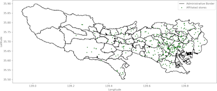
Fig. 1. Locations of orders in Tokyo.
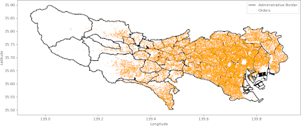
Fig. 2. Locations of affiliated stores in Tokyo.
3.6. Evaluation Metrics
The empirical experiments were evaluated in terms of average distance and store scale.
-
Average distance: The average Haversine distance per order between each delivery destination and the affiliated store to which the order is assigned.
-
Store scale: Spearman’s rank correlation coefficient between the peak-season capacity (\(\displaystyle C_i\)) and the actual number of orders assigned to each affiliated store.
As shorter delivery distances are desirable, the performance was evaluated using the average distance.
In addition, the store scale was employed as an evaluation metric to evaluate the extent to which orders were assigned considering store scale. As mentioned in Section 3.2.1, when operators balance order volumes across affiliated stores, the peak-season capacity (\(\displaystyle C_i\)) is referred to as the store scale. Validation using Spearman’s rank correlation coefficient revealed a strong positive correlation between each affiliated store’s peak-season capacity (\(\displaystyle C_i\)) and the actual number of orders assigned to each affiliated store by the operator. Therefore, the same metric was applied to the order assignment results to evaluate the extent to which each method considered store scale.
4. Results
Empirical experiments were conducted using the MW-Voronoi diagram and Huff model, as defined in Section 3. The results are presented for the following four cases to facilitate a comparison with the actual performance of the operator and existing methods:
-
The MW-Voronoi diagram (Section 3.2.1).
-
The Huff model (Section 3.2.2).
-
Manual assignment of the operator.
-
Voronoi diagram based solely on the Haversine distance.
Table 2. Results of the order assignment (top 1 store is considered in the Huff model).

Table 3. Results of the order assignment (top 5 stores are considered in the Huff model).

In the Huff model, the results depend on how many of the top-ranked stores according to \(P(O_{xi})\) are considered as candidates for assignment. First, we restricted the assignment to only the top 1 affiliated store, and Table 2 shows the results when the value of \(\lambda\) is varied from 0.2 to 2.0 in increments of 0.2. In the tables, the MW-Voronoi diagram is denoted as “MW-Voronoi,” the Huff model as “\(\lambda = \alpha\),” the operator’s manual assignments as “Operators,” and the Voronoi diagram based solely on distance without weights as “Voronoi.”
As evident from Table 2, the MW-Voronoi diagram outperformed the operator in terms of the average distance but performed worse in terms of the store scale. In contrast, the Huff model showed better performance than the operator’s results in both metrics when \(\lambda = 0.2\), \(0.4\), and \(0.6\), whereas for \(\lambda \geq 0.8\) it performed worse in terms of the store scale. “Voronoi” showed the best performance in terms of the average distance but the worst in terms of the store scale.
Furthermore, a comparison between the MW-Voronoi diagram and the Huff model showed that the results were identical in terms of both the average distance and store scale when \(\lambda = 1.0\). For \(\lambda > 1.0\), the Huff model performed better than the MW-Voronoi diagram in terms of the average distance but performed worse in terms of the store scale. In contrast, for \(\lambda < 1.0\), it performed worse in terms of the average distance but performed better in terms of the store scale.
Subsequently, Table 3 presents the results in which the top 5 affiliated stores, according to the Huff model’s choice probability \(P(O_{xi})\), were considered candidate stores. Table 4 presents the results in which the top 10 affiliated stores were considered. The experiments were conducted with \(\lambda = 1\), where the results were identical to those of the MW-Voronoi diagram in the case of the top 1 affiliated store, and with \(\lambda\) values from 2.0 to 10.0, increased in increments of 2.0. For ease of comparison, the results of “Operators,” “MW-Voronoi,” and “Voronoi” are also included in the tables.
Table 4. Results of the order assignment (top 10 stores are considered in the Huff model).

From Tables 3 and 4, it is evident that, as the number of candidate stores ranked by \(P(O_{xi})\) increases, both the average distance and store scale take larger values for the same value of \(\lambda\). In addition, it can be seen that for \(\lambda \geq 4.0\), both the average distance and store scale perform worse than “MW-Voronoi.”
5. Discussions
According to the results, the MW-Voronoi diagram and Huff model coincide when \(\lambda = 1\), whereas their relative performance diverges for \(\lambda \neq 1\). This result is consistent with the relationship between the MW-Voronoi diagram and Huff model discussed in Section 2.3. Empirical experiments revealed a trade-off between delivery efficiency (average distance) and store scale. The Huff model is advantageous because it allows \(\lambda\) to be adjusted to balance this trade-off depending on the operational objective. Thus, the Huff model has the advantage that it can be further refined to accommodate a specific problem context. Moreover, by adjusting the number of top-ranked stores considered in the choice probability \(P(O_{xi})\), the model provides flexibility for distributing orders across multiple affiliated stores.
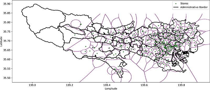
In contrast, the MW-Voronoi diagram has advantages. As a geometric method, it allows the visualization of the spatial extent of each Voronoi cell. Fig. 3 shows the Voronoi cells obtained from “MW-Voronoi,” and Fig. 4 shows those obtained from “Voronoi.” Figs. 3 and 4 show which affiliated stores have large territories. Conversely, they also reveal stores with almost no territory, and therefore gain little advantage from the affiliation.
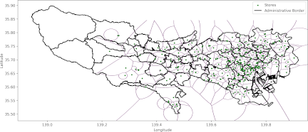
Fig. 3. MW-Voronoi diagram for affiliated stores.
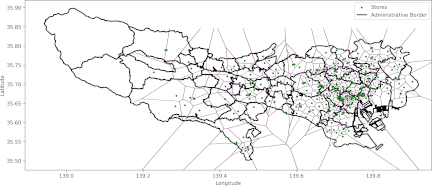
Fig. 4. Voronoi diagram for affiliated stores.
Therefore, both models have distinct strengths, and it is desirable to choose between them based on the characteristics and objectives of the problem context.
Note that the average delivery distance and its correlation with store scale do not fully reflect the operational performance in practice. Ensuring workload stability across affiliated stores is critical for real-world order assignments. The MW-Voronoi diagram yields a deterministic assignment that facilitates stable staffing and capacity planning. In contrast, the Huff model introduces variability because of its probabilistic assignment. Such stochasticity may pose operational risks, such as temporary overload at specific stores. Thus, actual operations may require variance-aware management, including workload standardization over time. Therefore, although the Huff model offers theoretical flexibility, its practical application should explicitly account for these uncertainties to maintain operational stability.
6. Conclusion
This study verified the relationship between the MW-Voronoi diagram and the Huff model.
First, we presented a theoretical comparison of the two models. This comparison showed that, when only the top-ranked candidate store based on the choice probability \(P(O_{xi})\) was selected, the MW-Voronoi diagram and Huff model yielded identical results.
Subsequently, empirical experiments were conducted using real-world data obtained from an EC platform provider. In these experiments, the Huff model was examined using various parameter settings. The results confirmed that orders assigned to the affiliated store with the highest choice probability \(P(O_{xi})\) were identical to the results of the MW-Voronoi diagram at \(\lambda = 1\). When the choice probability \(P(O_{xi})\) was extended to the top 5 or 10 affiliated stores, the Huff model, in some cases, showed worse performance than the MW-Voronoi diagram for both the average distance and store scale. The results of the empirical experiments demonstrated the flexibility of the Huff model in terms of parameter adjustment. In contrast, the MW-Voronoi diagram was advantageous because it enabled a geometric visualization of the delivery areas covered by each affiliated store. This comparison indicated that the MW-Voronoi diagram and the Huff model should be applied selectively depending on the characteristics and objectives of the problem context.
In future studies, three important directions should be identified. First, the essential difference between the MW-Voronoi diagram and the Huff model is that the former is deterministic, whereas the latter is probabilistic. Further theoretical developments are required to address this gap. In particular, constructing a probabilistic Voronoi diagram reflecting the choice probabilities of the Huff model is a promising approach. Second, it is necessary to evaluate the workload stability across affiliated stores from an operational perspective. Probabilistic assignments, such as the Huff model, may cause short-term fluctuations in realized order volumes. This may also lead to temporary overload at specific stores. Future studies should incorporate stability-related performance measures that capture the variability in store-level order volumes across planning periods. Variance-aware management systems should also be developed, such as standardizing the workload over time. Third, both the MW-Voronoi diagram and Huff model are currently formulated with a single measure of attractiveness. Therefore, it is necessary to develop models that incorporate multiple attractiveness factors to better reflect the complex decision-making processes in practical operations.
- [1] G. Voronoi, “Nouvelles applications des paramètres continus à la théorie des formes quadratiques. Premier mémoire. Sur quelques propriétés des formes quadratiques positives parfaites,” J. für die reine und angewandte Mathematik, Vol.1908, No.133, pp. 97-102, 1908. https://doi.org/10.1515/crll.1908.133.97
- [2] F. Aurenhammer, “Voronoi diagrams—A survey of a fundamental geometric data structure,” ACM Computing Surveys, Vol.23, No.3, pp. 345-405, 1991. https://doi.org/10.1145/116873.116880
- [3] A. Okabe, B. Boots, K. Sugihara, and S. N. Chiu, “Spatial Tessellations: Concepts and Applications of Voronoi Diagrams,” John Wiley & Sons, 1992.
- [4] D. L. Huff, “A probabilistic analysis of shopping center trade areas,” Land Economics, Vol.39, No.1, pp. 81-90, 1963. https://doi.org/10.2307/3144521
- [5] D. L. Huff, “Defining and estimating a trading area,” J. of Marketing, Vol.28, No.3, pp. 34-38, 1964. https://doi.org/10.2307/1249154
- [6] Y. Liang, S. Gao, Y. Cai, N. Z. Foutz, and L. Wu, “Calibrating the dynamic Huff model for business analysis using location big data,” Trans. in GIS, Vol.24, No.3, pp. 681-703, 2020. https://doi.org/10.1111/tgis.12624
- [7] R. Suárez-Vega, J. L. Gutiérrez-Acuña, and M. Rodríguez-Díaz, “Locating a supermarket using a locally calibrated Huff model,” Int. J. of Geographical Information Science, Vol.29, No.2, pp. 217-233, 2015. https://doi.org/10.1080/13658816.2014.958154
- [8] T. G. Lin, J. C. Xia, T. P. Robinson, D. Olaru, B. Smith, J. Taplin, and B. Cao, “Enhanced Huff model for estimating Park and Ride (PnR) catchment areas in Perth, WA,” J. of Transport Geography, Vol.54, pp. 336-348, 2016. https://doi.org/10.1016/j.jtrangeo.2016.06.011
- [9] J. A. Jeličić, M. Rapaić, M. Kapetina, S. Medić, and D. Ecet, “Urban planning method for fostering social sustainability: Can bottom-up and top-down meet?,” Results in Engineering, Vol.12, Article No.100284, 2021. https://doi.org/10.1016/j.rineng.2021.100284
- [10] B. Boots and R. South, “Modeling retail trade areas using higher-order, multiplicatively weighted Voronoi diagrams,” J. of Retailing, Vol.73, No.4, pp. 519-536, 1997. https://doi.org/10.1016/S0022-4359(97)90033-6
- [11] H. Tamagawa, “The implications of using a gravity model to determine territory in a circular domain,” Procedia – Social and Behavioral Sciences, Vol.21, pp. 167-176, 2011. https://doi.org/10.1016/j.sbspro.2011.07.009
- [12] T. Drezner, “A review of competitive facility location in the plane,” Logistics Research, Vol.7, Article No.114, 2014. https://doi.org/10.1007/s12159-014-0114-z
- [13] A. H. Thiessen, “Precipitation averages for large areas,” Monthly Weather Review, Vol.39, No.7, pp. 1082-1089, 1911. https://doi.org/10.1175/1520-0493(1911)39%3C1082b:PAFLA%3E2.0.CO;2
- [14] P. Dong, “Generating and updating multiplicatively weighted Voronoi diagrams for point, line and polygon features in GIS,” Computers & Geosciences, Vol.34, No.4, pp. 411-421, 2008. https://doi.org/10.1016/j.cageo.2007.04.005
- [15] H. Alani, C. B. Jones, and D. Tudhope, “Voronoi-based region approximation for geographical information retrieval with gazetteers,” Int. J. of Geographical Information Science, Vol.15, No.4, pp. 287-306, 2001. https://doi.org/10.1080/13658810110038942
- [16] M. Dai, F. Dong, and K. Hirota, “Fuzzy three-dimensional Voronoi diagram and its application to geographical data analysis,” J. Adv. Comput. Intell. Intell. Inform., Vol.16, No.2, pp. 191-198, 2012. https://doi.org/10.20965/jaciii.2012.p0191
- [17] Z. Miao, Y. Chen, X. Zeng, and J. Li, “Integrating spatial and attribute characteristics of extended Voronoi diagrams in spatial patterning research: A case study of Wuhan City in China,” ISPRS Int. J. of Geo-Information, Vol.5, No.7, Article No.120, 2016. https://doi.org/10.3390/ijgi5070120
- [18] Z. Sui, Y. Wen, C. Zhou, X. Huang, Q. Zhang, Z. Liu, and M. A. Piera, “An improved approach for assessing marine traffic complexity based on Voronoi diagram and complex network,” Ocean Engineering, Vol.266, Article No.112884, 2022. https://doi.org/10.1016/j.oceaneng.2022.112884
- [19] R. Hettiarachchi and J. F. Peters, “Multi-manifold-based skin classifier on feature space Voronoï regions for skin segmentation,” J. of Visual Communication and Image Representation, Vol.41, pp. 123-139, 2016. https://doi.org/10.1016/j.jvcir.2016.09.011
- [20] R. Hettiarachchi and J. F. Peters, “Voronoï region-based adaptive unsupervised color image segmentation,” Pattern Recognition, Vol.65, pp. 119-135, 2017. https://doi.org/10.1016/j.patcog.2016.12.011
- [21] S. Takumi and S. Miyamoto, “Nearest prototype and nearest neighbor clustering with twofold memberships based on inductive property,” J. Adv. Comput. Intell. Intell. Inform., Vol.17, No.4, pp. 504-510, 2013. https://doi.org/10.20965/jaciii.2013.p0504
- [22] S. Ide, S. Sumitsuji, O. Yamaguchi, and Y. Sakata, “Cardiac computed tomography-derived myocardial mass at risk using the Voronoi-based segmentation algorithm: A histological validation study,” J. of Cardiovascular Computed Tomography, Vol.11, No.3, pp. 179-182, 2017. https://doi.org/10.1016/j.jcct.2017.04.007
- [23] L. C. Galvão, A. G. N. Novaes, J. E. Souza de Cursi, and J. C. Souza, “A multiplicatively-weighted Voronoi diagram approach to logistics districting,” Computers & Operations Research, Vol.33, No.1, pp. 93-114, 2006. https://doi.org/10.1016/j.cor.2004.07.001
- [24] M. Wang, R. Ou, and Y. Wang, “Multiplicatively weighted Voronoi-based sensor collaborative redeployment in software-defined wireless sensor networks,” Int. J. of Distributed Sensor Networks, Vol.18, No.3, Article No.15501477211069903, 2022. https://doi.org/10.1177/15501477211069903
- [25] J. Kim, C. Ju, and H. I. Son, “A Multiplicatively Weighted Voronoi-Based Workspace Partition for Heterogeneous Seeding Robots,” Electronics, Vol.9, No.11, Article No.1813, 2020. https://doi.org/10.3390/electronics9111813
- [26] M. De Beule, D. Van den Poel, and N. Van de Weghe, “An extended Huff-model for robustly benchmarking and predicting retail network performance,” Applied Geography, Vol.46, pp. 80-89, 2014. https://doi.org/10.1016/j.apgeog.2013.09.026
- [27] I. Marić, A. Siljeg, F. Domazetovic, L. Pandja, R. Milosevic, S. Siljeg, and R. Marinovic, “How to delineate urban gravitational zones? GIS-based multicriteria decision analysis and Huff’s model in urban hierarchy modeling,” Papers in Regional Science, Vol.103, No.2, Article No.100015, 2024. https://doi.org/10.1016/j.pirs.2024.100015
- [28] S. Wang, N. N. Kong, and Y. Gao, “Use mobile location data to infer airport catchment areas and calibrate Huff gravity model in the New York metropolitan area,” J. of Transport Geography, Vol.114, Article No.103790, 2024. https://doi.org/10.1016/j.jtrangeo.2023.103790
- [29] L. Bello, R. Blanquero, and E. Carrizosa, “On minimax-regret Huff location models,” Computers & Operations Research, Vol.38, No.1, pp. 90-97, 2011. https://doi.org/10.1016/j.cor.2010.04.001
- [30] R. Blanquero, E. Carrizosa, B. G.-Tóth, and A. Nogales-Gómez, “p-facility Huff location problem on networks,” European J. of Operational Research, Vol.255, No.1, pp. 34-42, 2016. https://doi.org/10.1016/j.ejor.2016.04.039
- [31] S. Grohmann, D. Urošević, E. Carrizosa, and N. Mladenović, “Solving multifacility Huff location models on networks using metaheuristic and exact approaches,” Computers & Operations Research, Vol.78, pp. 537-546, 2017. https://doi.org/10.1016/j.cor.2016.03.005
- [32] B. G.-Tóth, L. Anton-Sanchez, and J. Fernández, “A Huff-like location model with quality adjustment and/or closing of existing facilities,” European J. of Operational Research, Vol.313, No.3, pp. 937-953, 2024. https://doi.org/10.1016/j.ejor.2023.08.054
- [33] T. Kawamoto and T. Hasuike, “A practical order assignment method to affiliated stores using Huff’s model,” IEEJ Trans. on Electronics, Information and Systems, Vol.144, No.8, pp. 742-748, 2024 (in Japanese). https://doi.org/10.1541/ieejeiss.144.742
- [34] T. Kawamoto and T. Hasuike, “Application of Analytic Hierarchy Process for order assignment to affiliated stores,” Proc. of the 2024 16th IIAI Int. Congress on Advanced Applied Informatics (IIAI-AAI), pp. 572-577, 2024. https://doi.org/10.1109/IIAI-AAI63651.2024.00109
- [35] T. Kawamoto and T. Hasuike, “Dynamic order assignment methods to affiliated stores using Voronoi tessellation,” Communications of the Operations Research Society of Japan, Vol.67, No.11, pp. 619-630, 2022 (in Japanese).
This article is published under a Creative Commons Attribution-NoDerivatives 4.0 Internationa License.