Research Paper:
Multi-Scale Fusion Fuzzy Method for Accurate and Interpretable Prediction of Photovoltaic Power Generation
Yixuan Yu, Chenlu Tian, Wei Peng
 , Yi Yan, and Chengdong Li†
Shandong Provincial Key Laboratory of Smart Buildings and Energy Efficiency, School of Information and Electrical Engineering, Shandong Jianzhu University
No.1000 Fengming Road, Licheng District, Jinan 250101, China
†Corresponding author

Photovoltaic (PV) power systems can provide clean, carbon-free energy and have become an important pathway for achieving carbon neutrality goals. Accurate prediction of PV power output is crucial for the rational scheduling and allocation of solar power resources. To further enhance the prediction accuracy at some local regions, especially around the peak or bottom points, this paper proposes a novel fusion fuzzy model for PV power forecasting. This model begins with the development of a distributed function-weighted fuzzy method (DFWFM), which effectively simplifies the structure of traditional fuzzy systems and significantly reduces the number of fuzzy rules. And an iterative regularized least squares method is developed for tuning the parameters of the DFWFM. Furthermore, a data-driven multi-scale fusion model (DMFM) is proposed to alleviate local prediction errors by training additional local models with data from high-error regions. The construction processes for such a multi-scale fusion model are also provided. Finally, detailed experiments are conducted, comparing the DFWFM-DMFM with five other prediction models. Experimental and comparative results demonstrate that this strategy substantially enhances the prediction accuracy in specific local areas, thereby improving the overall performance of the forecasting model.
Learning flowchart of the proposed DMFM
1. Introduction
1.1. Background
For many years, the global energy structure has predominantly relied on non-renewable fossil fuels. However, with the increasing severity of resource depletion and environmental pollution, countries worldwide have progressively shifted their focus towards developing low-carbon and even zero-carbon renewable energy sources 1,2. Currently, new energy generation has secured a significant share within global power systems 3. Among these, photovoltaic (PV) power generation stands out for its cost-effectiveness, high efficiency, and abundant resource base, establishing itself as a prominent form of renewable distributed energy worldwide. Furthermore, the rise of the “net zero carbon” and “carbon neutral” concepts has accelerated the rapid advancement of distributed PV technologies 4,5. Distributed PV systems involve the installation of relatively small-scale PV power generation units near end users, allowing for local electricity consumption and integration of surplus electricity into the grid, thereby alleviating the supply pressure on the grid 6. However, PV power generation is highly susceptible to fluctuations due to external meteorological changes, which can lead to voltage variations and localized power quality issues during grid integration, affecting the stability of the power system 7. Achieving accurate forecasting of PV power generation would enable better utilization of solar energy and more efficient scheduling and allocation of electrical resources 8.
1.3. Motivations and Contributions
Improving prediction accuracy is often achieved by either increasing the number of input variables or using hybrid models that combine various types of models. However, in traditional fuzzy methods, an excessive number of input variables can result in an exceedingly complex model structure, leading to issues such as an overabundance of training parameters and difficulties in training, and it may even cause rule explosion. This elucidates the reason for the limited application of fuzzy methods in multi-variable PV power forecasting tasks, despite their considerable interpretability.
In addition, all of the aforementioned studies focused primarily on the global prediction performance of the models. Although some methods were proposed to enhance prediction accuracy, their improvements are typically assessed from a global perspective, often overlooking the potentially significant local prediction errors, especially at some peak or valley points.
To simplify the fuzzy model structure and decrease large local prediction errors commonly faced in PV power forecasting, this paper first proposes a distributed function-weighted fuzzy method (DFWFM), and then develops a data-driven multi-scale fusion model (DMFM). The primary innovations and contributions of this study are as follows:
-
To address the rule explosion problem commonly encountered in traditional fuzzy methods, this study proposes the DFWFM. For each input variable, a single-input fuzzy module (SIFM) is constructed. The output of the DFWFM is determined based on the outputs of these SIFMs and the corresponding multivariate functional weights. This approach can significantly reduce the number of fuzzy rules, and can simplify the model structure.
-
To assure the forecasting performance, one iterative learning method is presented for the DFWFM. In this method, the regularized least squares method is employed to train the functional weights and consequent parameters in the fuzzy rules iteratively. Furthermore, the regularization mechanism in this learning method can effectively help to reduce the risk of overfitting.
-
To address the issue of substantial local prediction errors, a DMFM is developed. After training a global DFWFM, a distinctive encoding mechanism is established to identify and mark regions with significant errors. Data from these regions are then used to train local DFWFMs. The DMFM is constructed by combining the global model with these local models. The DMFM improves the global model performance by enhancing local prediction accuracy. To the best of the authors’ knowledge, this is the first time to focus on the local prediction errors in PV forecasting.
-
The proposed model was applied to two real-world PV power prediction scenarios, with detailed comparisons provided. Experimental results demonstrate that the model offers the best prediction performance when considering both training speed and accuracy, thereby validating the effectiveness of this model in PV power forecasting.
The remainder of the paper is organized as follows. In Section 2, the proposed DFWFM is introduced. In Section 3, the proposed DMFM is presented. In Section 4, two experiments are conducted and compared. Finally, the conclusions are presented in Section 5.
2. Distributed Functionally-Weighted Fuzzy Method
In the traditional fuzzy inference systems such as ANFIS, the “rule explosion” problem is often encountered. The number of fuzzy rules in ANFIS or traditional fuzzy models is determined by the combination of all the membership functions of the input variables. Specifically, if the input variables are \(\mathbf{x} = (x_1, x_2, \dots, x_n)\) and each input variable has \(m\) fuzzy sets, the total number of fuzzy rules will be \(m^n\). This implies that as the number of input variables increases in PV power forecasting, the total number of fuzzy rules in traditional fuzzy systems grows exponentially, leading to an increasingly complex model structure. This complexity results in longer training times and higher computational costs, and can cause difficulties in system convergence or even render the system inoperable.
In this section, we present a distributed fuzzy method with a modular structure.
2.1. Structure of the Proposed DFWFM
In this DFWFM, a SIFM is independently constructed for each input variable. The output of each SIFM is then weighted and integrated to obtain the total output of the DFWFM.
For each input variable \(x_i\), the fuzzy rules of the corresponding \(\mathit{SIFM}\)-\(i\) can be represented as
where \(m\) represents the number of fuzzy rules in the \(\mathit{SIFM}\)-\(i\); \(A_i^1, A_i^2, \dots, A_i^m\) denote the fuzzy sets for the variable \(x_i\); \(c_i^1, \dots, c_i^m\) and \(d_i^1, \dots, d_i^m\) are the consequent parameters in the consequent parts of the fuzzy rule \(R_i^1, R_i^2, \dots, R_i^m\).
Utilizing the singleton fuzzification and weighted defuzzification methods, the fuzzy inference output of \(\mathit{SIFM}\)-\(i\) can be expressed as
where \(\mu_{A_i^j}\) is the membership degree reflecting the extent to which the element \(x_i\) belongs to the fuzzy set \(A_i^j\).
The final output \(\hat y\left( {\mathbf{x}} \right)\) of the DFWFM is obtained by weighting and aggregating the outputs of the \(n\) SIFMs, and can be expressed as
where \({\omega _i}\left( {\mathbf{x}} \right) = \omega _i^0 + \omega _i^1{x_1} + \dots + \omega _i^n{x_n}\) is a multivariable function of \(\mathbf{x} = (x_1, x_2, \dots, x_n)\), which represents the dynamic weight or dynamic significance of the \(\mathit{SIFM}\)-\(i\).
Since each SIFM is a standalone single-input single-output fuzzy model and each input variable has \(m\) fuzzy sets, the number of fuzzy rules of DFWFM is \(m \times n\). Consequently, DFWFM can effectively reduce the number of rules in multi-variable fuzzy time series prediction tasks.
2.2. Data-Driven Design of the Proposed DFWFM
In this subsection, a detailed parameter learning method based on the regularized least square is provided.
2.2.1. Mathematical Formulation of the Parameters
The parameter vector for the functional weights of all SIFMs can be expressed as
The parameter vector for the consequent parameters in the fuzzy rules of all SIFMs can be expressed as
From Eq. (3), the input–output mapping of the DFWFM can be rewritten as
where \(g({\bf{x}},{\bf{c}}) = [ y({x_1}), {x_1}y({x_1}), \dots ,{x_n}y({x_1}), \dots ,y({x_n}),\) \({x_1}y({x_n}), \dots ,{x_n}y({x_n}) ]^{\rm{T}}\).
Alternatively, the input–output mapping of the DFWFM can also be rewritten as
where
2.2.2. Parameter Learning Based on the Regularized Least Squares Method
Assuming there are \(L\) input–output data pairs \(({\mathbf{x}}^1, {y^1}), ({\mathbf{x}}^2, {y^2}), \dots, ({\mathbf{x}}^L, {y^L})\) in the training data set, where \({{\mathbf{x}}^l} = ( {x_1^l,x_2^l, \dots ,x_n^l} )\), theoretically, the optimal solutions for the functional weights and the consequent parameters in the fuzzy rules of the DFWFM can be determined by the least squares method. The loss function for the least squares method can be expressed as
where \(\hat y( {{{\mathbf{x}}^l},{\mathbf{w}},{\mathbf{c}}} )\) represents the inference output of the DFWFM, and \(y^l\) is the actual output.
However, in practical applications, it becomes evident that using only the least squares method to determine the optimal solution of the model can make it susceptible to multicollinearity and overfitting. Multicollinearity can cause instability in the regression coefficients, resulting in poor prediction performance on new data. Similarly, overfitting can diminish the model’s generalization capability. To address these issues, the L2 regularization constraint is always adopted in the parameter learning of the DFWFM.
The L2 constraint limits the magnitude of the regression coefficients by adding a regularization term to the loss function, which smooths the coefficients and thereby can reduce overfitting to the training data. This enhances the model’s prediction performance on new data. Incorporating the L2 regularization constraint, the loss function expression according to Eq. (6) can be rewritten as
where
Alternatively, according to Eq. (7), incorporating the L2 regularization constraint, the loss function expression can also be rewritten as
where
It is challenging to simultaneously determine the optimal solutions for \(\mathbf{w}\) and \(\mathbf{c}\) that minimize the loss function. However, as shown in Eq. (9), if the parameter vector \(\mathbf{c}\) is known, the optimal solution for the parameter vector \(\mathbf{w}\) can be determined. Similarly, as indicated in Eq. (12), if the parameter vector \(\mathbf{w}\) is known, the optimal solution for the parameter vector \(\mathbf{c}\) can be found. Therefore, the optimal solutions for \(\mathbf{w}\) and \(\mathbf{c}\) can be sequentially determined by alternately solving the following equations:
and
Based on the derived formulas, we propose a data-driven iterative learning algorithm to learn the parameters of DFWFM. The specific iterative learning process is outlined in Algorithm 1 in pseudocode format.

3. The Data-Driven Multi-Scale Fusion Model
In this section, the proposed DMFM is described in detail. First, the overall process of the proposed model is introduced. Subsequently, the specific construction process for the local models within the DMFM is outlined. Finally, the method for combining the global model and local models in the DMFM is provided.
3.1. Overall Process of the Proposed DMFM
As previously mentioned, the global prediction performance improvements are often achieved by increasing the number of input variables or by combining different models. However, these methods are not entirely suitable for enhancing PV power prediction. This is because, during prediction, significant deviations often occur during peak periods of concentrated PV power generation. Ignoring these critical periods of prediction error and focusing solely on global model improvements make it difficult to achieve precise PV power forecasts. Therefore, to address the issue of substantial prediction errors in peak regions and other local areas during PV power forecasting, this section proposes the DMFM, which focuses on enhancing both the global and local prediction performance. The overall process of the proposed DMFM, based on the DFWFM, is illustrated in Fig. 1 and involves the following main steps:
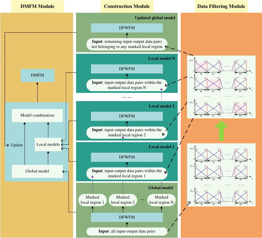
Fig. 1. The learning flowchart of the proposed DMFM.
-
Step 1: Train the DFWFM using the PV power dataset to establish a global model.
-
Step 2: Develop a partitioning mechanism for the input space, dividing the complete input space into a series of local input regions.
-
Step 3: Compare the global model’s predictions with actual values to identify and label local regions with poor prediction performance.
-
Step 4: Use the training data from the labeled local regions to train local DFWFMs, while updating the global DFWFM with the training data that were not labeled.
-
Step 5: Combine the local DFWFMs with the updated global DFWFM to form the DMFM.
The following subsections provide a detailed implementation methodology for these steps.
3.2. Input Space Partitioning
The input space partitioning of the global DFWFM consists of a set of non-overlapping intervals 44. The input domain of variable \(x_i\) can be divided into \(m-1\) regions by the \(m\) fuzzy sets, as illustrated in Fig. 2, where \({\mathbf{P}}_i^{k_i}\) (\(i = 1,2, \dots, n; k_i = 1, 2, \dots, m-1\)) represents the input domain corresponding to the \(k\)-th partition of the input variable \(x_i\).
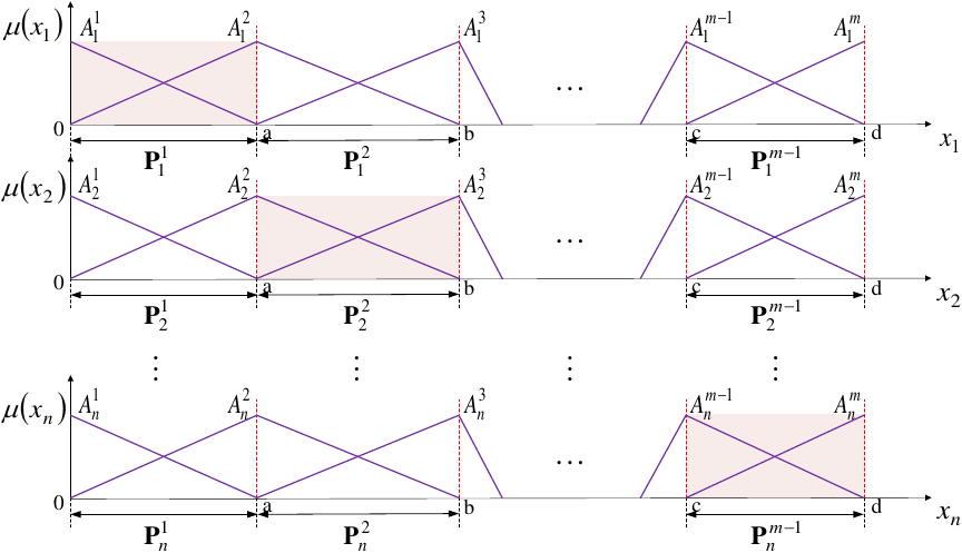
Fig. 2. Partitions of the input spaces for \(\mathbf{x}\).
Let \({{\mathbf{P}}^{{k_1},{k_2}, \dots ,{k_n}}}\) denote the set of the local input domains \({\mathbf{P}}_i^{{k_i}}\left( {i = 1,2, \dots ,n} \right)\). In other words, \({{\mathbf{P}}^{{k_1},{k_2}, \dots ,{k_n}}}\) can be represented as:
where \({k_i} = 1,2, \dots ,m - 1\), \(i = 1,2, \dots ,n\).
It is worth noting that each input \({\mathbf{x}} = ( {{x_1},{x_2}, \dots ,{x_n}} )\) should belong to only one local input domain \({{\mathbf{P}}^{{k_1},{k_2}, \dots ,{k_n}}}\).
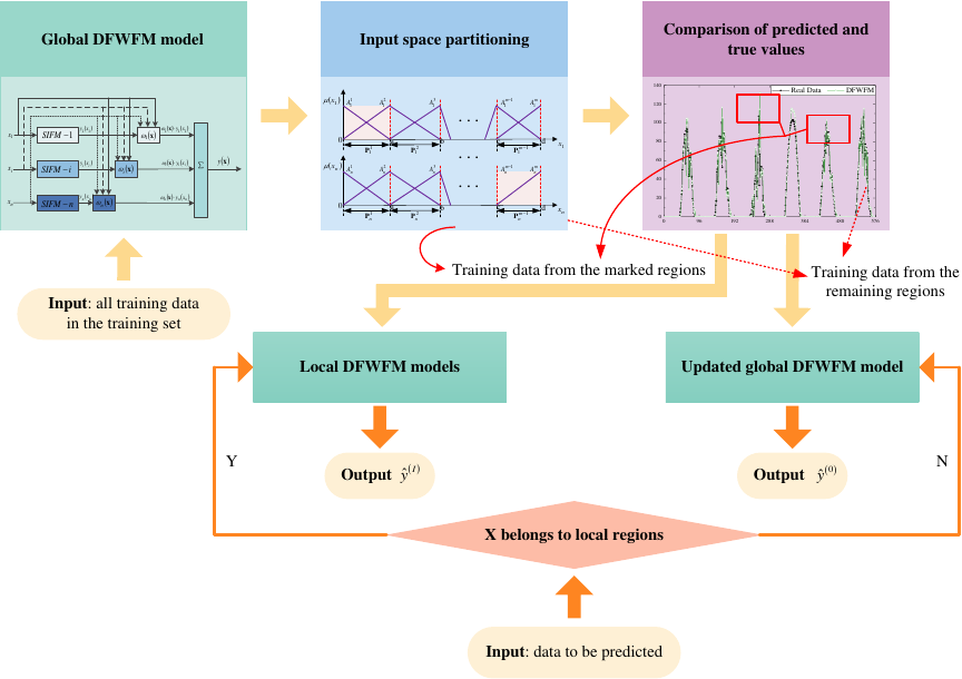
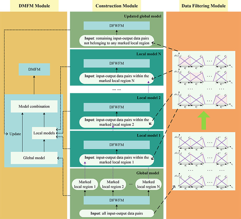
Fig. 3. The flowchart of the proposed DMFM.
3.3. Fusion of the Global and Local DFWFMs
In the global DFWFM, some regions often exhibit substantial errors, indicating that the existing fuzzy rules may not be suitable for predicting the PV power in these local regions. The proposed DMFM identifies the training data within these high-error regions and retrains new fuzzy rules based on these data patterns to construct corresponding local DFWFMs. Subsequently, the remaining training data are used to update the global DFWFM. In essence, the proposed DMFM is a combination of local models and the updated global model. The flowchart for constructing the DMFM based on the DFWFM is illustrated in Fig. 3. Detailed steps are as follows:
-
Step 1: Utilize the global DFWFM to predict the PV power.
-
Step 2: Calculate the sum of squared errors (SSE) for the training data in all \({\rm{P}}^{k_1,k_2,\dots,k_n}\) (\(k_i = 1, 2, \dots, m-1; i = 1,2,\dots,n\)). The SSE is employed to quantify the discrepancy between the predicted values and the actual values of the DFWFM, which is given by \(\mathit{SSE} = \sum{l = 1}^L {{{ ( {\hat y^l - y^l} )}^2}}\), where \(L\) denotes the total number of input–output data pairs, \({\hat y^l}\) represents the predicted value, and \(y^l\) denotes the true value.
-
Step 3: Sort the SSE results in the descending order, and the top \(N\) values of SSEs correspond to the local input domains that need to be marked.
-
Step 4: Label the training data that fall into the \(N\) local input domain ranges.
-
Step 5: Train the \(N\) local models using the labeled training data, and utilize the remaining training data, which do not fall into any local model and have not been labeled, to update the global model.
-
Step 6: If \(\mathbf{x}\) is within the local input domain of the \(I\)-th local model, the corresponding local model is employed to make the prediction, yielding the predicted value \({\hat y^{\left( I \right)}}\). Conversely, if \(\mathbf{x}\) does not fall within the input domain range of any local model, the updated global model is used for prediction, resulting in the predicted value \({\hat y^{\left( 0 \right)}}\). In other words, the final predicted output of DMFM can be computed as \begin{equation} \label{eq:17} \hat y\left( {\bf{x}} \right) = \left\{ {\begin{array}{*{20}{l}} {{{\hat y}^{\left( I \right)}}},\\ {{{\hat y}^{\left( 0 \right)}}}, \end{array}} \right. \end{equation}where \({{\hat y}^{\left( I \right)}}\) represents \({\bf{x}}\) that falls into the \(I\)-th local input domain \({\left( {I = 1,2, \dots ,N} \right)}\), \({{{\hat y}^{\left( 0 \right)}}}\) represents \({\bf{x}}\) that does not fall into the \(N\) local input domains.
4. Experiments and Comparisons
In this section, we first introduce the comparative models and evaluation metrics. Then, we provide the datasets for each experiment and the settings of the comparative models. Finally, detailed results and analyses are given.
4.1. Comparative Methods
To demonstrate the superiority of the proposed model, we select ANFIS, fuzzy neural network (FNN), support vector regression (SVR), back propagation neural network (BPNN) , and GRU as the comparative models. We now provide a brief overview of such comparative methods.
ANFIS is a hybrid model that integrates fuzzy inference systems with neural networks 45. It utilizes the neural network framework to extract fuzzy rules from data through an adaptive hybrid algorithm, continuously adjusting the antecedent and consequent parameters of the rules to obtain the optimal solution. ANFIS combines the advantages of fuzzy inference systems and neural networks while addressing their individual limitations, making it one of the most commonly used fuzzy time series prediction models today.
FNN is a hybrid model that integrates fuzzy logic with neural networks 46. It first fuzzifies the input data and then applies fuzzy rules for inference, making it well-suited for handling complex tasks characterized by uncertainty and vagueness. The FNN not only possesses the learning capabilities of neural networks but also benefits from the strong interpretability of fuzzy logic, which makes it widely used in fields such as control and prediction.
SVR is a variant of SVM, specifically designed for regression problems 47. SVR excels in handling high-dimensional feature spaces and nonlinear regression, demonstrating significant advantages in these areas. Additionally, it exhibits strong robustness in the presence of noise and outliers, making it widely applicable in fields such as time series forecasting.
BPNN is one of the most fundamental neural network structures 48, capable of approximating any continuous nonlinear function. As the complexity of the network architecture increases, BPNN can learn more intricate features, thereby addressing more complex problems. However, it is important to be cautious of overfitting due to excessive parameters. BPNN is among the most commonly used neural networks and finds extensive application in areas such as speech processing and time series forecasting.
GRU is an advanced variant of RNN 49, specifically designed for handling sequential data. By incorporating update and reset gates, GRU effectively retains crucial information over extended sequences while reducing the number of parameters. As a significant variation of RNN, GRU excels in applications such as natural language processing and time series forecasting.
4.2. Evaluation Indices
The forecasting performance of all models is evaluated using three metrics: the mean absolute error (MAE), the root mean squared error (RMSE), and the coefficient of determination (\({R^2}\)). The formulas for calculating these metrics are as follows:
Lower values of MAE and RMSE suggest that the predicted values are closer to the actual values, thereby indicating superior prediction performance of the model. The \({R^2}\) value ranges from 0 to 1, with values closer to 1 reflecting greater prediction accuracy.
4.3. PV Generation Prediction Without Meteorological Factors
4.3.1. Applied Dataset
In this experiment, we utilize the PV power plant data from the comprehensive power dataset of the microgrid at the University of California, San Diego 50. We select the PV generation data from February 1, 2019 to February 5, 2020 (a total of 370 days) for training and testing. The sampling interval for the dataset is 15 minutes. The dataset contains a total of 35,576 rows of data, with the first 24,056 rows used for training and the remaining 11,520 rows for validation.
4.3.2. Configuration of the Prediction Models
Since only the fuzzy models possess the concept of fuzzy sets, enabling the partitioning of regions based on the triggering of fuzzy rules, the SVR-, BPNN-, and GRU-based DMFMs require a pre-specified partitioning method. The \(K\)-means clustering algorithm is employed to divide the domain \({x_i}\) into \(K\) non-overlapping clusters, each represented by a unique cluster center, denoted as \({p_i}\) (\({i = 1,2, \dots ,K}\)). Using \(K\) intervals to mimic the partitioning domains as shown in Fig. 2, the domain of the input variable is divided into \(K+1\) regions as \([\min(x_i), p_1], [p_1, p_2], \dots, [p_{K-1}, p_K], [p_K, \max(x_i)]\).
In this experiment, all prediction models have four input variables and one output variable. In other words, the historical PV generation data from the previous four time intervals are used as four input variables to predict the future PV power generation. The DFWFM adopts the triangular membership functions, with each input variable having four fuzzy sets, and the iteration epoch is set to be 5. The parameter settings for the other comparative models are as follows:
-
In the ANFIS model, triangular membership functions are used, with each input variable having four fuzzy sets. And the learning iteration is set to be 60.
-
In the FNN model, triangular membership functions are also utilized, with each input variable having four fuzzy sets. The training is conducted using the quasi-Newton optimization algorithm, with a maximum of \(2 \times {10^5}\) function evaluations.
-
In the SVR model, the radial basis function kernel is employed for the nonlinear mapping of input features. During parameter selection, a grid search method is used to find the optimal configuration within the ranges of the penalty coefficient \(C\) and the kernel function parameter \(\gamma\), with \(C\) and \(\gamma\) varying between \([ {{2^{ - 3}},{2^3}} ]\). The loss function tolerance is set to be 0.8, and the termination criterion for allowable error is 0.01.
-
In the BPNN model, the number of neurons in the hidden layer is set to be 40, and the maximum number of training epochs is 2,000.
-
In the GRU model, the convolutional layers are configured with 32 and 64 kernels, the fully connected layers with 16 and 64 neurons, and the GRU layers with 50 GRU units. The initial learning rate is set to be 0.01, and the maximum number of iterations is 200.
In the SVR, BPNN, and GRU models, the input variable partitioning is performed using the \(K\)-means clustering algorithm, with two cluster centers set for each input variable.
4.3.3. Experimental Results and Comparative Analysis
In this experiment, the number of local models in the DMFM is set to be 0, 1, 2, or 3, respectively. When the number of local models is set to be 0, it indicates that there is only one global model with no local models, meaning all input variables fall within the domain of the global model. In this case, the prediction models are the traditional ones. Additionally, LM1, LM2, and LM3 are used to represent the scenarios with 1, 2, and 3 local models, respectively.
To demonstrate the improvement performance of the proposed model, Table 1 lists the MAE, RMSE, \({R^2}\) for each model during both training and testing phases, along with the training time and the number of fuzzy rules (NoFR) or neuro nodes (NoNN).
Table 1. Comparison of the prediction models in the first experiment.

From Table 1, it can be evident that compared to other fuzzy models, DFWFM consistently exhibits the fastest training speed and the fewest fuzzy rules. Moreover, this model maintains relatively optimal prediction performance across various numbers of local models. This indicates that the proposed model structure is relatively simple, allowing it to reduce model complexity while preserving prediction accuracy.
Additionally, Table 1 shows that as the number of local models in the DMFM increases, the training performance of the six prediction models improves. At the same time, since each additional local model requires the fuzzy rules or neuro nodes of the original base model to be retrained, the computational resource consumption also increases. From a theoretical perspective, in the absence of computational resource constraints, increasing the number of local models should further enhance the prediction performance of the DMFM. However, as shown in Table 1, nearly every model exhibits optimal testing or generalization performance when the number of local models in the DMFM is set to be 2, and further increasing the number of local models may actually degrade the model’s generalization performance or testing accuracy. This may be due to the atypical nature of PV power generation data or insufficient data for training local models, leading to overfitting.
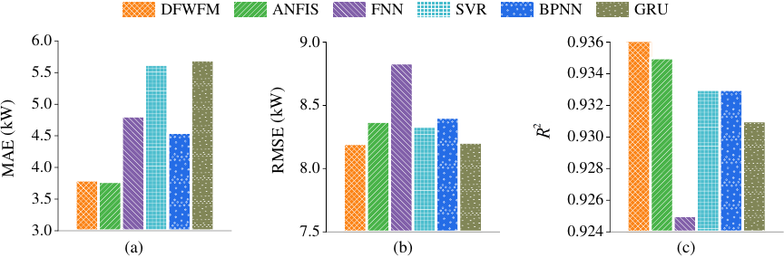
Fig. 4. Evaluation metrics of the six prediction models in the first experiment: (a) MAE, (b) RMSE, (c) \({R^2}\).
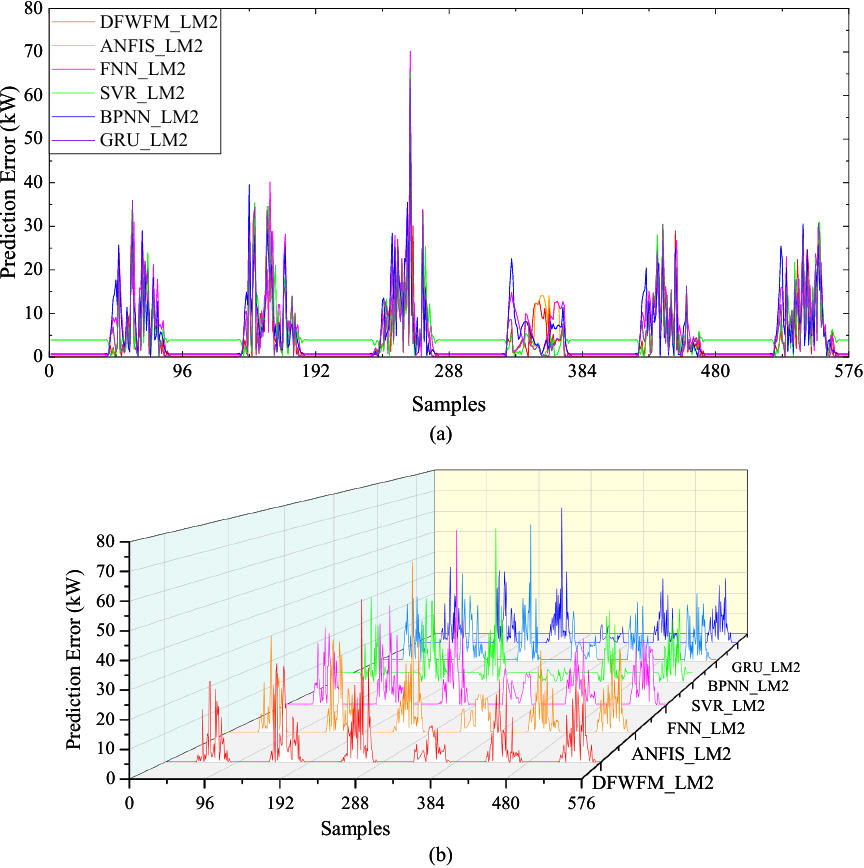
Fig. 5. Part of the prediction errors of the six prediction models in the first experiment: (a) two-dimensional form, (b) three-dimensional form.
Figure 4 illustrates the evaluation metrics of the six prediction models when two local models are employed. It can be observed from this figure that the DFWFM has nearly the smallest MAE and RMSE values, as well as an \({R^2}\) value that is closest to 1. This indicates that the DFWFM demonstrates superior prediction performance among the assessed models.
Figure 5 presents part of the prediction errors of the six prediction models using two local models, displayed in both two-dimensional and three-dimensional forms. The prediction errors in this figure represent the absolute differences between the predicted data and the real data at each sample point. From this, we can observe that after considering local models, all prediction models exhibit relatively small prediction errors. Furthermore, it is clear from this figure that the maximum prediction error of DFWFM_LM2 is significantly lower than that of the other models, indicating that the proposed model has better prediction performance.
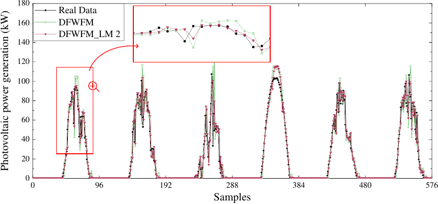
Fig. 6. Part of the prediction results of DFWFM-DMFM in the first experiment.
To intuitively demonstrate the superiority of the proposed method in reducing local prediction errors, Fig. 6 presents part of the prediction results of the DFWFM-DMFM. As can be observed, compared to using only the global model, adding extra local models can significantly reduce local prediction errors, particularly around peak points where the predicted values are closer to the actual values. This indicates that the proposed model can capture the dynamics of PV power generation more accurately.
Table 2. Comparison of the prediction models in the second experiment.

4.4. PV Power Generation Prediction Considering Meteorological Factors
4.4.1. Applied Dataset
In this experiment, PV power generation data from Arizona State University’s Tempe campus were utilized, which can be downloaded from the official ASU website: http://cm.asu.edu/. The dataset spans from March 16, 2023 to February 26, 2024 (a total of 347 days) and includes both PV power generation data and meteorological data. The samples in the dataset are recorded at hourly intervals. After employing linear interpolation to preprocess missing and anomalous values, the dataset contains 8,344 rows. The first 5,464 rows are used for training, while the remaining 2,880 rows are reserved for validation.
4.4.2. Configuration of the Prediction Models
In this experiment, 10 input variables-comprising the current meteorological data (ambient temperature, surface solar radiation, direct normal solar radiation, and diffuse solar radiation) and the historical PV power generation data from the previous six time steps-are used to predict future PV power generation. The parameter settings for the DMFM based on DFWFM, ANFIS, FNN, SVR, BPNN, and GRU are identical to those used in the previous experiment.
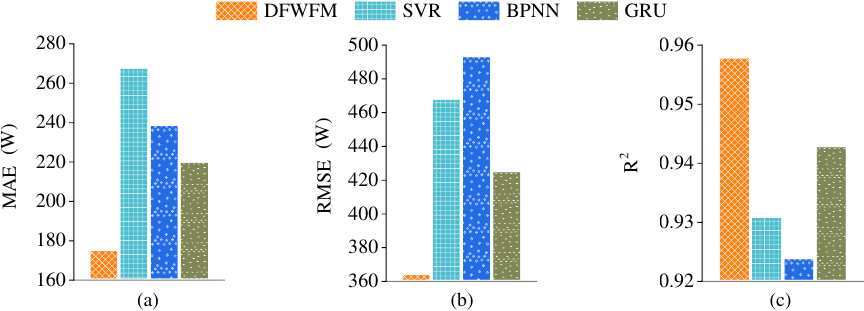
Fig. 7. Evaluation metrics of the four prediction models in the second experiment: (a) MAE, (b) RMSE, (c) \({R^2}\).
4.4.3. Experimental Results and Comparative Analysis
To illustrate the enhanced performance of the proposed models, Table 2 presents the MAE, RMSE, \({R^2}\) for each model during both training and testing phases, along with the training time and the NoFR or NoNN.
It is noteworthy that the number of input variables involved in this experiment has significantly increased, with all prediction models having 10 input variables and one output variable. ANFIS and FNN encountered a “rule explosion” problem due to the large number of fuzzy rules generated by the 10 input variables, which led to training failures for these models.
Table 2 shows that DFWFM consistently exhibits relatively fast training speed and optimal prediction performance in every case. Notably, its number of fuzzy rules is significantly lower than that of ANFIS and FNN. This indicates that increasing the number of input variables enhances the prediction performance of DFWFM without compromising the model’s structure. Therefore, for high-dimensional input prediction tasks, DFWFM is more suitable than traditional fuzzy inference methods.
The output power of PV systems is influenced by various meteorological factors. Accurately integrating these meteorological data allows for a more precise simulation of the actual generation environment, thereby significantly enhancing the accuracy of the prediction models. Neglecting these meteorological factors could result in predictions that deviate more significantly from reality. Thus, the inclusion of meteorological factors is one of the key reasons for the absence of overfitting in this case.
Compared to the first experiment, this one additionally incorporates meteorological data. From Table 2, it is evident that the performance of all models in both training and testing significantly improves with the increasing number of local models in DMFM. Specifically, the MAE and RMSE values for each model decrease progressively on both the training and test sets, while the \({R^2}\) values increase correspondingly. When the number of local models in the DMFM is set to be 3, nearly every model demonstrates optimal prediction performance.
Figure 7 presents the evaluation metrics for the four prediction models utilizing three local models. It is apparent that the DFWFM exhibits the best prediction performance.
Figure 8 presents part of the prediction errors of the four prediction models using three local models, displayed in both two-dimensional and three-dimensional forms. It can be observed that all prediction models considering local models exhibit relatively small prediction errors. Furthermore, the maximum prediction error of DFWFM is significantly lower than that of the other models.
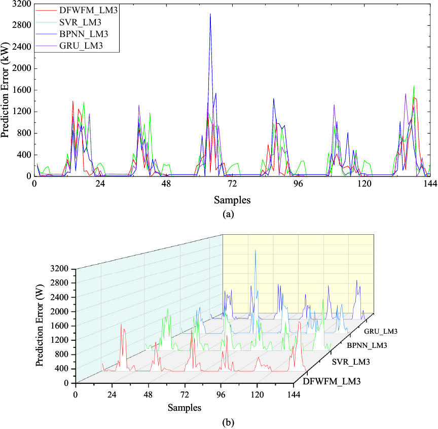
Fig. 8. Part of the prediction errors of the four prediction models in the second experiment: (a) two-dimensional form, (b) three-dimensional form.
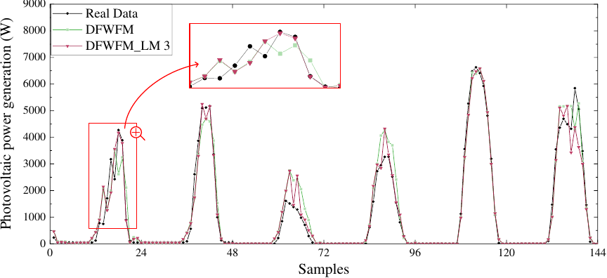
Fig. 9. Part of the prediction results of DFWFM-DMFM in the second experiment.
To intuitively demonstrate the superiority of the proposed method, Fig. 9 presents part of the prediction results of the DFWFM-DMFM with three additional local models. As can be observed, the DMFM with three local models aligns more closely with the actual values, particularly showing a significant reduction in prediction errors in the peak regions. This further validates the effectiveness of additional local models in enhancing local prediction accuracy.
4.5. In-Depth Analysis of the DMFM
4.5.1. Interpretability of the DFWFM
A model or system can be defined as interpretable if it presents its decision-making process and outcomes in a manner comprehensible to humans. For instance, linear models exhibit interpretability because their coefficients clearly characterize the linear influence of input variables on the output results. Moreover, fuzzy models provide a transparent reasoning process by utilizing fuzzy rules to articulate the relationships between inputs and outputs, thereby enhancing decision interpretability.
After the learning of the DFWFM-DMFM, all fuzzy rules constructed in the global and local DFWFMs can be obtained. The fuzzy models in the first and the second experiments are listed in Tables 3 and 4, respectively.
Table 3. The fuzzy rules in the constructed DFWFM-DMFM in the first experiment.

Table 4. The fuzzy rules in the constructed DFWFM-DMFM in the second experiment.

By examining the activation strengths of these fuzzy rules presented in these two tables, we can accurately comprehend the activation effects of each fuzzy rule. The triggered rules and the data that activated the corresponding rules can be clearly displayed, providing valuable insights. Furthermore, the parameters within the fuzzy rules can also be interpreted through fuzzy or qualitative knowledge. This further substantiates the strong interpretability of the proposed DFWFM-DMFM.
4.5.2. Selection of the Number of Local Models
During the development of the DMFM, the number of local models plays a crucial role in the performance of the overall model. Determining the number of local models not only affects how DMFM covers and divides the input space, but also directly influences the overall complexity of the DMFM.
The number \(N\) of local models in DMFM cannot be arbitrarily large. The common approach is to first determine a reasonable range for \(N\), and then select the most appropriate value within that range based on the verification error criterion. By default, the specific steps for choosing the number \(N\) of local models are as follows:
-
Step 1: Compute the global SSE of the training dataset and the SSE of each data partition.
-
Step 2: Count and record the number of partitions whose SSE exceeds the global SSE, denoted as \(s\). This number \(s\) represents the potential number of local input domains that need to be marked, which is the maximum possible value of the \(N\) of local models.
-
Step 3: Perform an exhaustive search for \(N \in \left\{ {1,2, \dots ,s} \right\}\) to determine which value of \(N\) gives the smallest error on the validation or test set, and then select the optimal value of \(N\).
4.5.3. Computational Complexity
In the in-depth analysis of the computational complexity of DMFM, we use big-O notation to describe its time complexity. It should be noted that big-O notation is inherently an abstract tool that reflects how an algorithm scales with increasing parameters and does not directly indicate actual running time. Therefore, we connect the theoretical time complexity with the actual training cost. Specifically, we use \(T\) to represent the training time of the model and examine how \(T\) changes as the number of local models increases, as shown in Tables 1 and 2, in order to gain an intuitive understanding of the growth trend described by big-O notation.
The computational cost of the DFWFM-DMFM mainly comes from training the global model and the local models. Using big-O notation, the time complexity of the DFWFM-DMFM can be written as
where, \(e\) is the number of epochs, \(p\) is the number of model parameters, and \(N\) is the number of local models. Since the pseudo-inverse of the parameter matrix needs to be computed, the overall complexity of DFWFM-FWFM is proportional to \({p^3}\).
It is worth noting that in Tables 1 and 2, the actual training time of some models increases approximately linearly with the number of local models, while others exhibit a non-strictly linear pattern. This is mainly due to the varying amounts of training data associated with each local model. When some local models have fewer samples, their training time contributes less to the overall increase. Overall, as the number of local models grows, the training time shows a general upward trend, which is consistent with the growth direction described by big-O theory.
5. Conclusion
In this study, a hybrid model for high-dimensional PV power forecasting is proposed. To address the challenge of fuzzy rule explosion in traditional fuzzy systems, we proposed the DFWFM. By independently constructing a SIFM for each input variable, the number of fuzzy rules can be significantly reduced, thereby simplifying the overall model structure. To tackle the issue of substantial errors in local regions during PV power forecasting, the DMFM is proposed. This approach constructs local models to enhance prediction accuracy in specific regions, thereby improving the overall model performance. The proposed hybrid model is applied to two practical PV power forecasting experiments. Experimental and comparative results validate the performance and advantages of the proposed method.
Despite the effectiveness of the DMFM has been verified, some limitations still remain. For instance, determining the optimal number of local models is challenging. An insufficient number of local models may not substantially improve the prediction performance, whereas an excessive number can lead to overfitting and significantly increase the training time. Future research will focus on exploring methods to identify the most suitable number of local models to balance the prediction accuracy with the training efficiency.
CRediT authorship contribution statement Yixuan Yu: Conceptualization, data curation, formal analysis, investigation, methodology, software, visualization, writing—original draft. Chenlu Tian: Conceptualization, funding acquisition, methodology, resources, supervision, writing—review and editing. Wei Peng: Funding acquisition, investigation, software, supervision. Yi Yan: Data curation, formal analysis, validation, visualization. Chengdong Li: Conceptualization, formal analysis, funding acquisition, methodology, project administration, writing—review and editing.
Data availability Data will be made available on request.
Declaration of competing interest The authors declare that they have no known competing financial interests or personal relationships that could have appeared to influence the work reported in this paper.
Acknowledgments
This study is partly supported by the National Natural Science Foundation of China (Nos.62133008, 62573272), the Key Research and Development Program of Shandong Province (No.2025CXPT076), the Natural Science Foundation of Shandong Province (ZR2023QF020), and the Projects for Universities and Colleges in Jinan (202228039, 202534104).
- [1] Z. Wang, Y. Wang, S. Cao, S. Fan, Y. Zhang, and Y. Liu, “A robust spatial-temporal prediction model for photovoltaic power generation based on deep learning,” Computers and Electrical Engineering, Vol.110, Article No.108784, 2023. https://doi.org/10.1016/j.compeleceng.2023.108784
- [2] D. Liu and K. Sun, “Random forest solar power forecast based on classification optimization,” Energy, Vol.187, Article No.115940, 2019.
- [3] Y. Li, P. Janik, and H. Schwarz, “Prediction and aggregation of regional PV and wind generation based on neural computation and real measurements,” Sustainable Energy Technologies and Assessments, Vol.57, Article No.103314, 2023. https://doi.org/10.1016/j.seta.2023.103314
- [4] H. Gao, S. Qiu, J. Fang, N. Ma, J. Wang, K. Cheng, H. Wang, Y. Zhu, D. Hu, H. Liu, and J. Wang, “Short-Term Prediction of PV Power Based on Combined Modal Decomposition and NARX-LSTM-LightGBM,” Sustainability, Vol.15, Issue 10, Article No.8266, 2023. https://doi.org/10.3390/su15108266
- [5] Q. Dai, X. Huo, Y. Hao, and R. Yu, “Spatio-temporal prediction for distributed PV generation system based on deep learning neural network model,” Frontiers in Energy Research, Vol.11, Article No.1204032, 2023. https://doi.org/10.3389/fenrg.2023.1204032
- [6] Y. Jiang, K. Fu, W. Huang, J. Zhang, X. Li, and S. Liu, “Ultra-short-term PV power prediction based on Informer with multi-head probability sparse self-attentiveness mechanism,” Frontiers in Energy Research, Vol.11, Article No.1301828, 2023. https://doi.org/10.3389/fenrg.2023.1301828
- [7] H. Song, N. Al Khafaf, A. Kamoona, S. S. Sajjadi, A. M. Amani, M. Jalili, X. Yu, and P. McTaggart, “Multitasking recurrent neural network for photovoltaic power generation prediction,” Energy Reports, Vol.9, Supplement 3, pp. 369-376, 2023. https://doi.org/10.1016/j.egyr.2023.01.008
- [8] H. Zhang, J. Shi, and C. Zhang, “A hybrid ensembled double-input-fuzzy-modules based precise prediction of PV power generation,” Energy Reports, Vol.8, Supplement 4, pp. 1610-1621, 2022. https://doi.org/10.1016/j.egyr.2022.02.298
- [9] P. Malik and S. S. Chandel, “A new integrated single-diode solar cell model for photovoltaic power prediction with experimental validation under real outdoor conditions,” Int. J. of Energy Research, Vol.45, No.1, pp. 759-771, 2021. https://doi.org/10.1002/er.5881
- [10] M. Kumar, P. Malik, R. Chandel, and S. S. Chandel, “Development of a novel solar PV module model for reliable power prediction under real outdoor conditions,” Renewable Energy, Vol.217, Article No.119224, 2023. https://doi.org/10.1016/j.renene.2023.119224
- [11] Y. Chaibi, A. Allouhi, M. Malvoni, M. Salhi, and R. Saadani, “Solar irradiance and temperature influence on the photovoltaic cell equivalent-circuit models,” Solar Energy, Vol.188, pp. 1102-1110, 2019. https://doi.org/10.1016/j.solener.2019.07.005
- [12] T. Villemin, O. Farges, G. Parent, and R. Claverie, “Monte Carlo prediction of the energy performance of a photovoltaic panel using detailed meteorological input data,” Int. J. of Thermal Sciences, Vol.195, Article No.108672, 2024. https://doi.org/10.1016/j.ijthermalsci.2023.108672
- [13] C. Li, C. Zhou, W. Peng, Y. Lv, and X. Luo, “Accurate prediction of short-term photovoltaic power generation via a novel double-input-rule-modules stacked deep fuzzy method,” Energy, Vol.212, Article No.118700, 2020. https://doi.org/10.1016/j.energy.2020.118700
- [14] Y. Chu, B. Urquhart, S. M. I. Gohari, H. T. C. Pedro, J. Kleissl, and C. F. M. Coimbra, “Short-term reforecasting of power output from a 48 MWe solar PV plant,” Solar Energy, Vol.112, pp. 68-77, 2015. https://doi.org/10.1016/j.solener.2014.11.017
- [15] J. Zhang, Z. Tan, and Y. Wei, “An adaptive hybrid model for day-ahead photovoltaic output power prediction,” J. of Cleaner Production, Vol.244, Article No.118858, 2020. https://doi.org/10.1016/j.jclepro.2019.118858
- [16] M. Trigo-González, F. J. Batlles, J. Alonso-Montesinos, P. Ferrada, J. Del Sagrado, M. Martínez-Durbán, M. Cortés, C. Portillo, and A. Marzo, “Hourly PV production estimation by means of an exportable multiple linear regression model,” Renewable Energy, Vol.135, pp. 303-312, 2019. https://doi.org/10.1016/j.renene.2018.12.014
- [17] Y. Li, Y. Su, and L. Shu, “An ARMAX model for forecasting the power output of a grid connected photovoltaic system,” Renewable Energy, Vol.66, pp. 78-89, 2014. https://doi.org/10.1016/j.renene.2013.11.067
- [18] E. Kim, M. S. Akhtar, and O.-B. Yang, “Designing solar power generation output forecasting methods using time series algorithms,” Electric Power Systems Research, Vol.216, Article No.109073, 2023. https://doi.org/10.1016/j.epsr.2022.109073
- [19] M. Bouzerdoum and A. Mellit, “Performance prediction of a grid-connected photovoltaic plant,” 2017 5th Int. Conf. on Electrical Engineering-Boumerdes (ICEE-B), 2017. https://doi.org/10.1109/ICEE-B.2017.8192059
- [20] M. Lotfi, M. Javadi, G. J. Osório, C. Monteiro, and J. P. Catalão, “A Novel Ensemble Algorithm for Solar Power Forecasting Based on Kernel Density Estimation,” Energies, Vol.13, Issue 1, Article No.216, 2020. https://doi.org/10.3390/en13010216
- [21] C. Li, M. Tang, G. Zhang, R. Wang, and C. Tian, “A Hybrid Short-Term Building Electrical Load Forecasting Model Combining the Periodic Pattern, Fuzzy System, and Wavelet Transform,” Int. J. of Fuzzy Systems, Vol.22, pp. 156-171, 2020. https://doi.org/10.1007/s40815-019-00783-y
- [22] T. Lu, Q. Ai, W.-J. Lee, Z. Wang, and H. He, “An Aggregated Decision Tree-Based Learner for Renewable Integration Prediction,” 2018 IEEE Industry Applications Society Annual Meeting (IAS), 2018. https://doi.org/10.1109/IAS.2018.8544544
- [23] C. Brester, V. Kallio-Myers, A. V. Lindfors, M. Kolehmainen, and H. Niska, “Evaluating neural network models in site-specific solar PV forecasting using numerical weather prediction data and weather observations,” Renewable Energy, Vol.207, pp. 266-274, 2023. https://doi.org/10.1016/j.renene.2023.02.130
- [24] L. Wang, Y. Liu, T. Li, X. Xie, and C. Chang, “The Short-Term Forecasting of Asymmetry Photovoltaic Power Based on the Feature Extraction of PV Power and SVM Algorithm,” Symmetry, Vol.12, Issue 11, Article No.1777, 2020. https://doi.org/10.3390/sym12111777
- [25] M. S. Hossain and H. Mahmood, “Short-Term Photovoltaic Power Forecasting Using an LSTM Neural Network and Synthetic Weather Forecast,” IEEE Access, Vol.8, pp. 172524-172533, 2020. https://doi.org/10.1109/ACCESS.2020.3024901
- [26] P. Li, K. Zhou, X. Lu, and S. Yang, “A hybrid deep learning model for short-term PV power forecasting,” Applied Energy, Vol.259, Article No.114216, 2020. https://doi.org/10.1016/j.apenergy.2019.114216
- [27] D. Lee and K. Kim, “PV power prediction in a peak zone using recurrent neural networks in the absence of future meteorological information,” Renewable Energy, Vol.173, pp. 1098-1110, 2021. https://doi.org/10.1016/j.renene.2020.12.021
- [28] R. Nelega, D. I. Greu, E. Jecan, V. Rednic, C. Zamfirescu, E. Puschita, and R. V. F. Turcu, “Prediction of Power Generation of a Photovoltaic Power Plant Based on Neural Networks,” IEEE Access, Vol.11, pp. 20713-20724, 2023. https://doi.org/10.1109/ACCESS.2023.3249484
- [29] F. Wang, Z. Xuan, Z. Zhen, K. Li, T. Wang, and M. Shi, “A day-ahead PV power forecasting method based on LSTM-RNN model and time correlation modification under partial daily pattern prediction framework,” Energy Conversion and Management, Vol.212, Article No.112766, 2020. https://doi.org/10.1016/j.enconman.2020.112766
- [30] Y. Jiang, L. Zheng, and X. Ding, “Ultra-short-term prediction of photovoltaic output based on an LSTM-ARMA combined model driven by EEMD,” J. of Renewable and Sustainable Energy, Vol.13, Issue 4, Article No.046103, 2021. https://doi.org/10.1063/5.0056980
- [31] J. Zhang, Z. Liu, and T. Chen, “Interval prediction of ultra-short-term photovoltaic power based on a hybrid model,” Electric Power Systems Research, Vol.216, Article No.109035, 2023. https://doi.org/10.1016/j.epsr.2022.109035
- [32] M. Tovar, M. Robles, and F. Rashid, “PV Power Prediction, Using CNN-LSTM Hybrid Neural Network Model. Case of Study: Temixco-Morelos, México,” Energies, Vol.13, Issue 24, Article No.6512, 2020. https://doi.org/10.3390/en13246512
- [33] Q. Dai, X. Huo, Y. Hao, and R. Yu, “Spatio-temporal prediction for distributed PV generation system based on deep learning neural network model,” Frontiers in Energy Research, Vol.11, Article No.1204032, 2023. https://doi.org/10.3389/fenrg.2023.1204032
- [34] L. A. Zadeh, “Fuzzy sets,” Information and Control, Vol.8, Issue 3, pp. 338-353, 1965. https://doi.org/10.1016/S0019-9958(65)90241-X
- [35] C. Li, J. Gao, J. Yi, and G. Zhang, “Analysis and Design of Functionally Weighted Single-Input-Rule-Modules Connected Fuzzy Inference Systems,” IEEE Trans. on Fuzzy Systems, Vol.26, Issue 1, pp. 56-71, 2016. https://doi.org/10.1109/TFUZZ.2016.2637369
- [36] M. Fujita and Y. Kanzawa, “Three Fuzzy c c-Shapes Clustering Algorithms for Series Data,” J. Adv. Comput. Intell. Intell. Inform., Vol.27, No.5, pp. 976-985, 2023. https://doi.org/10.20965/jaciii.2023.p0976
- [37] H. A. Calinao Jr., R. C. Gustilo, E. P. Dadios, and R. S. Concepcion II, “Enhancing Fault Detection and Classification in Grid-Tied Solar Energy Systems Using Radial Basis Function and Fuzzy Logic-Controlled Data Switch,” J. Adv. Comput. Intell. Intell. Inform., Vol.28, No.1, pp. 41-48, 2024. https://doi.org/10.20965/jaciii.2024.p0041
- [38] K. Liao, X. Li, C. Mu, and D. Wang, “Short-term photovoltaic power prediction based on T-S fuzzy neural network,” 2018 33rd Youth Academic Annual Conf. of Chinese Association of Automation (YAC), pp. 620-624, 2018. https://doi.org/10.1109/YAC.2018.8406448
- [39] C.-R. Chen, F. B. Ouedraogo, Y.-M. Chang, D. A. Larasati, and S.-W. Tan, “Hour-Ahead Photovoltaic Output Forecasting Using Wavelet-ANFIS,” Mathematics, Vol.9, Issue 19, Article No.2438, 2021. https://doi.org/10.3390/math9192438
- [40] M. Monfared, M. Fazeli, R. Lewis, and J. Searle, “Fuzzy Predictor With Additive Learning for Very Short-Term PV Power Generation,” IEEE Access, Vol.7, pp. 91183-91192, 2019. https://doi.org/10.1109/ACCESS.2019.2927804
- [41] N. Li, L. Li, F. Huang, X. Liu, and S. Wang, “Photovoltaic power prediction method for zero energy consumption buildings based on multi-feature fuzzy clustering and MAOA-ESN,” J. of Building Engineering, Vol.75, Article No.106922, 2023. https://doi.org/10.1016/j.jobe.2023.106922
- [42] J. Kim, G. Kim, W. Son, and G. Byeon, “Photovoltaic Output Prediction using Monotonic Fuzzy System,” 2018 IEEE 7th World Conf. on Photovoltaic Energy Conversion (WCPEC), pp. 2320-2324, 2018. https://doi.org/10.1109/PVSC.2018.8547625
- [43] D. M. Teferra, L. M. H. Ngoo, and G. N. Nyakoe, “Fuzzy-based prediction of solar PV and wind power generation for microgrid modeling using particle swarm optimization,” Heliyon, Vol.9, Issue 1, Article No.e12802, 2023. https://doi.org/10.1016/j.heliyon.2023.e12802
- [44] D. Wu and J. M. Mendel, “Patch learning,” IEEE Trans. on Fuzzy Systems, Vol.28, Issue 9, pp. 1996-2008, 2020. https://doi.org/10.1109/TFUZZ.2019.2930022
- [45] J.-S. R. Jang, “ANFIS: Adaptive-network-based fuzzy inference system,” IEEE Trans. on Systems, Man, and Cybernetics, Vol.23, Issue 3, pp. 665-685, 1993. https://doi.org/10.1109/21.256541
- [46] J. J. Buckley and Y. Hayashi, “Fuzzy neural networks: A survey,” Fuzzy Sets and Systems, Vol.66, Issue 1, pp. 1-13, 1994. https://doi.org/10.1016/0165-0114(94)90297-6
- [47] H. Drucker, C. J. C. Burges, L. Kaufman, A. Smola, and V. Vapnik, “Support vector regression machines advances,” Proc. of the 10th Int. Conf. on Neural Information Processing Systems (NIPS’96), pp. 155-161, 1996.
- [48] D. E. Rumelhart, G. E. Hinton, and R. J. Williams, “Learning representations by back-propagating errors,” Nature, Vol.323, No.6088, pp. 533-536, 1986. https://doi.org/10.1038/323533a0
- [49] R. Dey and F. M. Salem, “Gate-variants of gated recurrent unit (GRU) neural networks,” 2017 IEEE 60th Int. Midwest Symp. on Circuits and Systems (MWSCAS), pp. 1597-1600, 2017. https://doi.org/10.1109/MWSCAS.2017.8053243
- [50] S. Silwal, C. Mullican, Y.-A. Chen, A. Ghosh, J. Dilliott, and J. Kleissl, “Open-source multi-year power generation, consumption, and storage data in a microgrid,” J. of Renewable and Sustainable Energy, Vol.13, Issue 2, Article No.025301, 2021. https://doi.org/10.1063/5.0038650
This article is published under a Creative Commons Attribution-NoDerivatives 4.0 Internationa License.