Research Paper:
Prediction of Circulating Load Ratio for Semi-Autogenous Grinding Process Using Fuzzy C-Means and Bayesian-Optimized Random Forest
Zhenhong Liao*1,*2,*3,*4
 , Jinhua She*1,*5,†
, Yanglong Zhang*4, and Wen Chen*4
, Jinhua She*1,*5,†
, Yanglong Zhang*4, and Wen Chen*4
*1School of Automation, China University of Geosciences
No.388 Lumo Road, Hongshan District, Wuhan, Hubei 430074, China
*2Hubei Key Laboratory of Advanced Control and Intelligent Automation for Complex Systems
No.388 Lumo Road, Hongshan District, Wuhan, Hubei 430074, China
*3Engineering Research Center of Intelligent Technology for Geo-Exploration, Ministry of Education
No.300 Lumo Road, Hongshan District, Wuhan, Hubei 430074, China
*4Department of Mineral Resources Development and Utilization, Changsha Research Institute of Mining and Metallurgy Co., Ltd.
No.966 South Lushan Road, Yuelu District, Changsha, Hunan 410012, China
*5School of Engineering, Tokyo University of Technology
1404-1 Katakuramachi, Hachioji, Tokyo 192-0982, Japan
†Corresponding author

Grinding in mineral processing critically depends on real-time control of the circulating load ratio (CLR) to optimize efficiency and reduce energy consumption. While investigating the impact of the CLR on the grinding process from a mechanistic perspective can optimize production, it fails to achieve real-time perception of its dynamic variations during operation. This limitation hinders timely adjustments to operational parameters. Focusing on an actual semi-autogenous grinding (SAG) process, this paper presents a hybrid fuzzy C-means (FCM) and Bayesian-optimized random forest (BO-RF) framework that explicitly addresses nonlinearity and operational variability in the SAG process. Key parameters influencing CLR are first identified through mechanistic analysis. Operating conditions are clustered via FCM, followed by BO-RF submodel construction for each cluster. A nearest-neighbor criterion dynamically activates submodels for real-time prediction. Validated with industrial data from an iron concentrate plant, the method achieves more than 90% prediction accuracy. This approach establishes a generalizable framework for complex industrial processes with multivariate dynamics.
CLR modeling framework

1. Introduction
In mineral processing, it is necessary to liberate valuable minerals from other non-valuable components to efficiently concentrate these minerals by methods, such as magnetic separation, flotation, and leaching 1. Dispersed complex ores require sufficient crushing to liberate valuable minerals 2. Comminution, including crushing and grinding, is the process of reducing particle size in mining, mineral processing, and a range of other industries. Grinding takes place in a tumbling mill, such as AG, SAG, ball, and rod mills 3,4. It is achieved by the impact, abrasion, and wear of the ore by the free motion of unconnected media, such as steel rods, steel or ceramic balls, or coarse ore pebbles 5.
AG and SAG mills are used as primary grinding units, while ball and rod mills are used as secondary grinding units in large-scale plant operations 1. Industrial AG or SAG mills are primary grinding plants that receive their feed material directly from the crusher. The mills are difficult to control and stabilize due to the variable characteristics of the feed ore in terms of hardness and particle size distribution. In addition, other process parameters, such as mill speed, mill load, fresh-ore feed rate, water flow rate, and grinding time, can affect the overall performance of a mill 6. While it is possible to analyze ore size distribution with a vision system in an online fashion 7, ore hardness measurement is a time-consuming and laborious process and can be performed outside the grinding circuit 1. This, coupled with the fact that the grinding process is characterized by opacity, instability, and complex flow conditions 8, makes it difficult to achieve on-site observation of the internal behavior of the mill. As a result, it is often not possible to adjust the grinding process parameters in time to accommodate changes in ore properties and mill operating conditions.
The CLR is an important indicator for assessing the operating condition of a mill. Grinding in the mining industry is always done in a closed circuit, in which material of the desired size is removed by a classifier (spiral classifier, hydrocyclone, or screen) and oversize material is returned to the mill 9. The material returned to the mill by the classifier is called the circulating load. It is always expressed as a percentage of the weight of new feed material, namely CLR. The cause of the increase in CLR may be that the feed ore has become hard or the media and liners in the mill have changed. In either case, an operator should reduce the feed rate or adjust other parameters to avoid clogging the mill by accumulating more ore that has not been ground to the required size. Thus, the ability to predict the circulating load or CLR based on the current operating parameters of a milling process provides a new basis for making timely adjustments to the operating conditions of the mill.
Currently, most studies investigate the impact of CLR on production based on grinding processes and mechanisms. Wei et al. investigated the effects of circulating load and grinding feed on the grinding kinetics of cement clinker in an industrial mill and calculated the optimal operating area of an industrial mill for different circulating loads 10. Dündar examined the benefits of replacing hydrocyclones with high-frequency fine screens in a closed grinding circuit 11. The data showed a reduction in circulating loads, resulting in a 13% increase in throughput and a 15% reduction in grinding energy consumption. Li et al. presented a novel circulating load prediction method based on the principle of mass balance and first-order crushing kinetics 12. These studies have proven that CLR is an important parameter for evaluating mill operating conditions, which not only affect mill capacity, but also have a significant impact on mill product and the subsequent separation process. However, the grinding process is characterized by strong coupling between variables, high nonlinearity, and time-varying dynamics under different operating conditions 13,14. Although this mechanism-based approach is highly effective for process optimization, it is difficult to apply to the real-time prediction of CLR in actual dynamic production processes.
Machine learning methods have been extensively adopted in the mineral process industry 15, offering diverse methodological frameworks for constructing predictive models of CLR. For example, Liao et al. established a CLR model using BPNN and SVR 16. Since the grinding process is a complex system with multiple operating conditions, it is a feasible and effective solution to classify the SAG operating conditions and separately predict the CLR under different conditions. The rational classification of operating conditions means an effective decomposition of the complex characteristics of the SAG process and helps to reduce the complexity of the system. For example, Liao et al. used mill power and CLR as features and applied the \(K\)-means method to cluster SAG operating conditions 16. There are a lot of applications of this multi-model approach 17,18,19, usually combining clustering methods, such as FCM, WKFCM, with machine learning methods.
Fuzzy clustering is a commonly used method in industrial processes and has the advantages of fast computation, good stability, and easy online training 20,21,22. RF is a bagging-based ensemble method that aggregates multiple regression trees generated via bootstrapping 23. The RF handles both discrete and continuous variables without distributional assumptions, inherently resists overfitting 24,25, and reduces complexity through two mechanisms: (a) constructing submodels from bootstrap-sampled data subsets; (b) enabling parallel computation for efficient training. Its ensemble structure ensures robust performance while maintaining computational efficiency. Olivier and Aldrich used the RF to develop a decision support system for the control of a grinding circuit 26. Loudari et al. conducted a comparative assessment of KNN, RF, and XGBoost for predicting grinding mill power consumption 27. The results show that the RF model achieves superior predictive accuracy. Napier and Aldrich used an RF model as a predictor to estimate the particle size on an industrial IsaMill 28. Furthermore, the RF has also been successfully implemented in the simulation of an industrial grinding circuit 29 and prediction of mill throughput 30.
Therefore, based on the operational characteristics of the SAG process, this paper presents a hybrid method for predicting the CLR. A real-time CLR prediction model is established using a data-driven approach based on collected industrial production data. This method involves clustering SAG operating conditions using FCM, and then modeling the CLR with RF within each resulting cluster. By clustering the complex SAG process, multi-condition dynamics are decomposed to reduce process nonlinearity, thereby enhancing model accuracy. The model will provide an effective means for real-time dynamic prediction and adjustment of the CLR. The main contributions of this paper are as follows:
-
1)
A novel FCM clustering method for SAG operating conditions is presented through mechanism analysis and multisensory data fusion, explicitly handling nonlinear regime transitions.
-
2)
A dynamic BO-RF prediction model activated by nearest-neighbor criteria is developed to predict CLR under different operating conditions of an actual SAG process, achieving more than 90% prediction accuracy.
-
3)
The model framework provides different methodological options for modeling similar industrial processes.
The rest of this paper is organized as follows: Section 2 describes the SAG process and analyzes the operating mechanism and characteristics of the SAG process. Section 3 explains the approaches for predicting CLR. Section 4 presents the identification of operating conditions. Section 5 models the CLR and discusses the results. Section 6 presents some concluding remarks and future work.
2. Process Description and Mechanism Analysis
A typical SAG milling circuit (Fig. 1) was considered in this study. It mainly consists of grinding and screening.
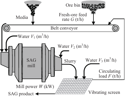
Fig. 1. Typical SAG milling process.
Fresh ore is fed from an ore bin onto a belt conveyor and then conveyed to the SAG mill. The steel balls are fed into the SAG mill along with the ore. The SAG mill utilizes the ore itself as part of the grinding media with the addition of steel balls as grinding media. Since the SAG milling is performed wet, water is added at the mill inlet. The ore and water are continuously rolled in the mill and mixed into a slurry. As the SAG mill rolls, the ore and media collide and crush inside the mill shell, resulting in a reduction in ore size. After the ore is ground, the slurry is discharged from the other end of the SAG mill and then into the vibrating screen. Water is added to dilute the slurry as it is discharged from the mill, as well as when it is screened. The screen is fitted with fixed-size meshes and classifies the slurry into coarser and finer particles by vibration. Ore with a particle size smaller than the sieve size is the product of the SAG mill. Ore with a particle size larger than the sieve size is conveyed by belt to the SAG mill for regrinding. The main variables that affect the CLR are fresh-ore feed rate (\(G\) [t/h]), water flowrate in SAG mill (\(V_1\) [m\(^3\)/h]), mill discharge water flowrate (\(V_2\) [m\(^3\)/h]), slurry flushing water flowrate (\(V_3\) [m\(^3\)/h]), mill power (\(W\) [kW]), circulating load (\(F\) [t/h]), and grinding media.
The CLR represents the ore that enters the SAG mill and is not ground to the desired size. It is usually expressed as a ratio or percentage of the fresh ore. According to the description of an SAG process, the amount of ore fed into an SAG mill at a given time \(t\) is the sum of \(G\) and \(F\). Field measurements and mechanism analysis indicate that the residence time of the ore in the SAG mill is 35 minutes. It takes 5 minutes to screen and recycle the circulating load back to the SAG mill. This implies the whole process time is 40 minutes. After classification, a new circulating load \((F^{\prime})\) is sent back to the SAG mill for regrinding after \((t + 40)\) minutes. As a result, the CLR is
The SAG process operates through precise regulation of three critical parameters: grinding concentration, mill charge, and mill power, which collectively ensure efficient ore comminution. Following primary grinding, the discharge undergoes classification using high-frequency vibrating screens. Qualified particles proceed to subsequent beneficiation stages, while oversized materials (circulating load) are recycled to the SAG mill for regrinding. This operational configuration achieves optimal dynamic equilibrium between throughput efficiency and product size distribution.
The grinding concentration, expressed as the solid-to-slurry weight percentage, is determined by \(G\), \(V_1\), and \(F\). Elevated grinding concentration increases slurry viscosity while reducing fluidity, thereby restricting grinding media kinetic energy and diminishing impact breakage efficiency. Conversely, excessive water content decreases particle-media collision frequency, lowering comminution effectiveness. The optimal density regime facilitates efficient particle size reduction to target specifications, generating balanced SAG product yields alongside controlled CLR.
The SAG mill’s total power consumption (\(W\)) comprises no-load power (accounting for frictional/mechanical losses) and net grinding power. The net power exhibits a nonlinear correlation with mill charge. The mixture of media, ore, and water in a mill is called the mill charge. As the mill charge continues to increase, the net power initially increases significantly. After reaching a critical value, the net power tends to decrease. Given the impracticality of real-time monitoring for grinding media weight within the mill, and considering the established nonlinear correlation between mill charge and power consumption, mill power serves as a proxy indicator for quantifying internal media mass.
Besides, slurry concentration critically affects screening efficiency. Elevated slurry concentration promotes particle entrainment, causing sub-sieve particles to agglomerate and resist dispersion. These agglomerates are retained on the screen surface, thereby entering the circulating load and inducing overgrinding. Consequently, regulation of \(V_2\) and \(V_3\) proves essential for stabilizing both slurry concentration and CLR.
The variables \(G\), \(F\), \(W\), \(V_1\), \(V_2\), and \(V_3\) were systematically selected as model inputs for CLR prediction based on the above process description and mechanism analysis.
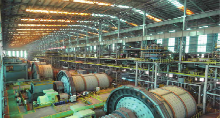
Fig. 2. The SAG circuit in a concentrate plant.
The original dataset of the SAG process at the production site (Fig. 2) was continuously acquired via installed sensors during March to May 2022. Temporal alignment was performed using process mechanism analysis to compensate for transport delays inherent in material flow dynamics. The input features representing the operating condition (\(G, W\), \(V_1\)) and the incoming \(F\) are aligned at the beginning of the cycle (time \(t\)). The mill discharge water flowrate (\(V_2\)) and slurry flushing water flowrate (\(V_3\)), which affect the slurry as it is discharged and screened, are aligned with a time shift of \(T_1\) = 35 minutes (i.e., \(V_{2}(t+T_1)\) and \(V_{3}(t+T_1)\)). The target variable, the CLR (\(C\)), is derived from the new circulating load \(F'\) that returns to the mill after the full 40-minute cycle. Therefore, it is calculated at time \(t+T\) (i.e., Eq. \(\eqref{eq:C}\)). The original time-series sensor data were systematically rearranged using this mechanistic timing model to compensate for the transport and process delays. The aligned data were then partitioned into non-overlapping 40-minute intervals. The average value of each variable within its respective aligned timeframe over these 40-minute windows was calculated to form a single, coherent data sample representing the process state. Missing data were imputed via linear interpolation. Outliers beyond 3\(\sigma\) were removed using Hampel filtering. This preprocessing yielded 2,900 validated samples for modeling.
3. Approach to CLR Prediction
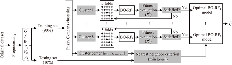
Since the SAG process is characterized by multiple operating conditions and multiple parameters, a clustering-based multimodel framework is developed for CLR prediction (Fig. 3).
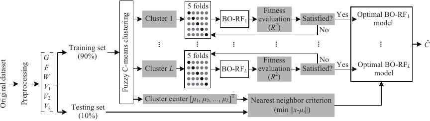
Fig. 3. CLR modeling framework.
The prediction of CLR is formulated as a multi-step-ahead forecasting problem within a state-space modeling framework. In this context, the circulating load \(F\) is treated not merely as an input feature, but as a key state variable representing the mill’s load condition at time. This approach allows the model to capture the dynamic evolution of the grinding process by integrating the current operational state with manipulable inputs (\(G\), \(W\), \(V_1\), \(V_2\), and \(V_3\)) to predict future CLR. This formulation aligns with industrial practice where \(F\) is both measurable and adjustable, thereby supporting realistic scenario analysis and feedforward control strategies.
First, the pre-processed data are randomly divided into a training set and a testing set, where the training set is 90% and the testing set is 10%. Then, the operating conditions are clustered in the training set. The model inputs for predicting CLR are used as the clustering features, and the FCM method is used to classify the operating conditions. Different operating conditions are identified, and different cluster centers are obtained. Model complexity is reduced by decomposing nonlinear dynamics into locally linear submodels via operating condition clustering, not by isolating individual variables.
Next, submodels for predicting the CLR are built using the RF in each operating condition. RF was selected for its robustness and practicality in modeling the SAG process. Its inherent noise resistance, achieved through bagging and random feature selection, is crucial for handling volatile industrial sensor data 23,25. Compared to gradient-boosting methods like XGBoost, RF offers greater computational efficiency via parallel training and is less sensitive to hyperparameter settings, simplifying model development 26. Furthermore, RF provides intrinsic feature importance measures, which validate our mechanistic analysis and enhance model interpretability 28. While boosters can achieve high accuracy, RF provides a superior balance of predictive stability, efficiency, and overfitting control for this dynamic industrial application. The RF model is constructed with initialization parameters.
Hyperparameters governing model architecture and training dynamics (e.g., learning rates, hidden layers, and activation functions) critically impact predictive performance 31. Hyperparameter optimization methods for machine learning span gradient descent, grid/random search, PSO, and Bayesian approaches. While gradient descent demonstrates efficacy in continuous differentiable spaces, its applicability diminishes for non-convex or non-differentiable optimization problems 32. Grid/random search strategies become computationally prohibitive in high-dimensional spaces due to exhaustive sampling requirements 33. PSO often exhibits premature convergence and suboptimal exploration–exploitation balance 34. BO addresses these limitations through adaptive surrogate modeling—typically GPs—that probabilistically maps the response surface, enabling sequential decision-making to minimize expensive function evaluations while balancing exploration and exploitation 35,36. The BO algorithm is employed to optimize the hyperparameters through a five-fold cross-validation process, with the maximum \(R^2\) of the five-fold cross-validation as the objective function.
Assuming that the operating conditions are classified into \(L\) clusters, there are \(L\) submodels of the BO-RF. When performing model evaluation, the nearest neighbor criterion is used to determine that the testing data belong to the \(i\)-th \((1 \leq i \leq L)\) cluster. The \(i\)-th BO-RF submodel is then invoked to predict the CLR. The criterion is the minimum Euclidean distance between the cluster centers (\(\mu_i, i=1,2,\dots, L\)) and the testing data. All the simulations were run on an Intel\(^{®}\) Xeon\(^{®}\) CPU Gold 6226R@2.90 GHz (2 processors) 256 GB RAM machine.
4. Clustering of Operating Condition
This section presents the FCM algorithm, clustering evaluation metrics, and results of operating condition clustering.
4.1. FCM Algorithm
The FCM clustering algorithm determines the categories of the sample points by optimizing the objective function and obtains the degree of membership of each sample point to the centers of all clusters 37. This achieves the purpose of classifying the sample data. Unlike hard clustering algorithms like \(K\)-means, which assign each data point to a single cluster, FCM’s soft clustering approach via membership degrees better captures the overlapping and gradual transitions between different operational states. This is more physically meaningful for a dynamic industrial process where boundaries between conditions are not always sharp.
Let \(X = \{ {{x_i}{ \in \mathbb{R}^6}|i = 1,2,\dots,n} \}\) denote the clustering features, where \(x_i = [G_i, F_i, W_i, V_{1i}, V_{2i}, V_{3i} ]^{\rm T}\), \(n\) is the number of sample data. Assume that \(X\) is classified into \(L\) (\(2 \le L \le n\)) clusters. Then \(V = \{ {{v_j}{ \in \mathbb{R}^6}|j = 1, 2, \dots, L} \}\) and \({v_j} = [ {{v_{1j}},{v_{2j}},\dots,{v_{6j}}} ]^{\rm T}\) represent the \(L\) cluster centers. The core idea of the FCM algorithm is to minimize the objective function, i.e., minimize the weighted squared error within clusters 38. The objective function is
Fuzzy clustering is achieved by iterative optimization of the above objective function with the update of membership \(\mu _{ji}\) and the cluster center \(v_j\). The update equations are as follows:
Then the optimal \(U\) and \(V\) are obtained. The cluster of each sample is determined from the matrix \(U\). In particular, a sample is assigned to the cluster with the largest corresponding membership value.
4.2. Results of Operating Clustering
PC, PE, and SiS are employed to evaluate the performance of clustering at different \(L\) values.
The larger the value of PC is, the better the clustering result is. Meanwhile, the optimal number of clusters is the one with the largest PC value. When PE is small, the partitioning uncertainty of the data is low, and the clustering performance of the data is good. SiS ranges from \(-1\) to 1. A high value (close to 1) indicates that the sample is well matched to its own cluster and poorly matched to neighboring clusters. The optimal number of clusters is the one that maximizes the average SiS.
We first set the range of \(L\) from 2 to 10. This ensures that the clustering reflects changes in the operating conditions without adding too much computational cost. Then, PC, PE, and SiS were calculated for different numbers of clusters (Fig. 4).
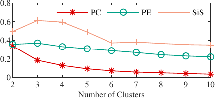
Fig. 4. PC, PE, and SiS values for different numbers of clusters.
The results show that the value of PC decreases with the increase in the number of clusters. This means that the centrality of clusters is weakening as the number of clusters increases, resulting in a worse clustering effect. The value of PE increases and then decreases with the increase of the number of clusters. It reaches the maximum at \(L = 3\). The value of SiS increases and then decreases with the increase of the number of clusters. It also reaches the maximum at \(L = 3\). PE and SiS gradually stabilize with the increase of the number of clusters. Therefore, the PC, PE, and SiS values are more variable when the number of clusters is 2 to 5, which is a more reasonable centrality and distributional balance of the data.
5. Prediction for CLR
This section first briefly describes the model algorithm, then presents the steps for Bayesian optimization of the hyperparameters of the models, next determines the optimal number of clusters, and finally shows the results of the different strategies and models for predicting the CLR.
5.1. RF Algorithm
RF is an ensemble learning method that combines multiple decision trees to improve predictive accuracy and control overfitting. A single decision tree splits the feature space into regions based on impurity metrics (e.g., Gini impurity for classification, mean squared error for regression) 39. However, individual trees are prone to overfitting and high variance.
RF employs bagging to reduce variance. Given a dataset \(D = \{ {{x_i},{y_i}} \}_{i = 1}^n\), generate \(B\) bootstrap samples \(D^{(1)}, D^{(2)}, \dots, D^{(B)}\), each of size \(n\), by sampling with replacement. Each \(D^{(b)}\) contains approximately 63.2% unique instances from \(D\). Approximately 36.8% of the original data samples are left out. These samples are not used for the training of the corresponding tree.
RF introduces additional randomness into the model by using a random subset of features at each split, thus further reducing correlation among trees and enhancing the variance reduction effect. For a dataset with a total number of features \(P\), \(m\) features (where \(m < P\)) are randomly selected for each splitting of the decision tree. This randomization reduces the correlation between decision trees and makes the ensemble more robust.
Each tree \(T_b\) is trained on \(D^{(b)}\). The process is repeated for each node until a stopping criterion is met, such as a maximum depth or a minimum sample count at a node. The prediction value \((\hat{y})\) for the input \(x\) is derived by averaging the predictions of all decision trees.
5.2. BO for Hyperparameter Tuning of RF
BO is a sequential model-based approach that minimizes an objective function \(f(X)\) by iteratively selecting hyperparameters \(X \in \aleph\), where \(\aleph\) is the search space. It comprises two core components: a surrogate model and an acquisition function.
A surrogate model is a probabilistic model. GPs are commonly used due to their flexibility in modeling uncertainty:
RF performance depends on several hyperparameters: number of trees (\(B\)_estimators), maximum depth (max_depth), features per split (max_features), minimum samples per split (min_samples_split), and minimum samples per leaf (min_samples_leaf). The BO workflow for RF includes the following four steps.
-
Step 1:
Define bounded ranges for each hyperparameter. \(B\)_estimators: (10, 200), max_depth: (2, 50); max_features: (0.1, 1.0); min_samples_split: (2, 20); min_samples_leaf: (1, 10).
-
Step 2:
Define the objective function. The objective function \(f(X)\) quantifies RF performance using cross-validated metrics.
-
Step 3:
Initialize surrogate model. Start with an initial set of \(N_\mathit{init}\) hyperparameter configurations. Evaluate \(f(X)\) for each configuration.
-
Step 4:
Iteratively optimize. For \(t = 1, 2, \dots, T_{\max }\), first, update surrogate model: fit the GP to all observed data. Then, select the next hyperparameters that maximize the acquisition function:
\begin{equation} X_t = \underset{X \in \aleph}{\arg\max}\, EI(X). \end{equation}Next, evaluate the objective function: train RF with \(X_t\) and compute \(f(X_t)\). Finally, update dataset: add \(((X_t), f(X_t))\) to observations. -
Step 5:
Return optimal configuration. After \(T_{\max}\) iterations, select
\begin{equation} X^* = \underset{X \in \{X_1, X_2, \dots, X_T\}}{\arg\min} F(X). \end{equation}
5.3. Performance Evaluation Metrics
Root mean square error (RMSE), mean absolute error (MAE), mean absolute percentage error (MAPE), coefficient of determination (\(R^2\)), and prediction error (Err) are employed to evaluate the performance of prediction models.
RMSE is a metric for evaluating the difference between predicted and actual values. MAE is the arithmetic mean of the absolute error. The closer the values of RMSE and MAE are to 0, the better the prediction performance of the modeling method used. MAPE is often used as a measure of the relative error of a prediction. \(R^2\) is a coefficient ranging from 0 to 1, and a larger \(R^2\) indicates a more effective prediction model. Err is the difference between the actual value and the predicted value.
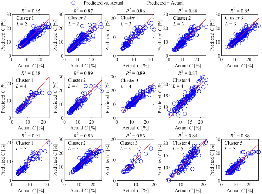
Fig. 5. Prediction results of BO-RF sub-models on the validation set for different numbers of clusters.
5.4. CLR Prediction
Since it is difficult to determine the optimal number of clusters based on the results of clustering, we used BO-RF to model each cluster when \(L\) ranges from 2 to 5. The number of clusters was determined by the prediction performance of the BO-RF submodel for CLR in each cluster (here we only took \(R^2\) as a validation metric for the submodels).
The submodel validation results (Fig. 5) demonstrate that when the cluster number \(L = 4\), all BO-RF submodels achieve \(R^2\) values above 0.86, with a maximum of 0.89. This indicates that BO-RF achieves an accurate prediction of CLR in each cluster. In contrast, configurations with \(L = 2\), 3, or 5 exhibit degraded performance in certain submodels, where \(R^2\) falls below 0.86. This decline becomes particularly pronounced at \(L = 5\), with two submodels yielding \(R^2\) values of only 0.83 and 0.84. Further analysis reveals that excessive \(L\) values lead to over-partitioned operational conditions, resulting in clusters with inadequate sample sizes and increased feature dispersion, thereby compromising model fitting efficacy. Based on comprehensive validation across all submodels, \(L = 4\) is identified as the optimal parameter configuration.
To validate the impact of cluster numbers on model performance and confirm the optimality of \(L=4\), experiments were conducted using testing set data across the cluster number range \(L=2\) to 5, following the framework illustrated in Fig. 3.
Results from the testing set (Table 1) demonstrate that the BO-RF model achieves its optimal performance at \(L = 4\), attaining the highest \(R^2\) (0.87) and the lowest error metrics: RMSE (0.0158), MAE (1.09%), and MAPE (9.98%). These results indicate a prediction accuracy exceeding 90% (derived from \(\mathrm{MAPE} <10\%\)) and MAE of only 1.09%. In contrast, configurations with \(L = 2\), 3, or 5 yield MAPE values above 10%, corresponding to sub-90% accuracy. The prediction results under the optimal cluster number \(L = 4\) (Fig. 6(a)) demonstrate strong agreement with actual values. The Errs are distributed within the range [\(-5.75\)%, 5.57%], with 93.44% of the error samples concentrated in the narrower interval [\(-3\)%, 3%] (Fig. 6(b)), demonstrating superior prediction stability of the model.
Table 1. Prediction performance of the BO-RF model with different numbers of clusters.

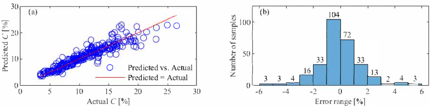
Fig. 6. Prediction results of BO-RF on the testing data at \(L = 4\). (a) Prediction results; (b) error distributions.
Wilcoxon signed-rank tests comparing the MAE distributions of \(L = 4\) against alternative configurations reveal a statistically significant difference when contrasted with both \(L = 2\) \((p = 0.039)\) and \(L = 3\) \((p = 0.033)\). However, no significant difference is found between \(L = 4\) and \(L = 5\) \((p = 0.231)\). It aligns with their similar mean MAE values (1.09% vs. 1.11%).
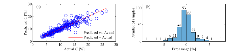
Fig. 7. Prediction results of BO-RF on the testing data without clustering. (a) Prediction results; (b) error distributions.
Table 2. Prediction performance of different models at \(L = 4\).

To comprehensively validate the efficacy of the FCM-based BO-RF method for CLR prediction, a dual-phase experimental framework was implemented.
-
(1)
Baseline modeling. A BO-RF model was established using the same training dataset to predict the CLR without considering the multi-operating conditions of the SAG process. The modeling performance was evaluated on the same testing set.
-
(2)
Multimodal comparison. Under the FCM-derived four-cluster operating classification, a cross-algorithm experiment was performed between BO-RF and four Bayesian-optimized models: BO-XGBoost, BO-GBDT, BO-SVR, and BO-BPNN.
The BO-RF directly modeling CLR without operating condition clustering achieved acceptable prediction accuracy (Fig. 7(a)), with 90.34% of Err distributed within [\(-3\)%, 3%] (Fig. 7(b)). Evaluation metrics yielded \(R^2 = 0.84\), \(\mathrm{RMSE} = 0.0174\), \(\mathrm{MAE} = 1.19\%\), and \(\mathrm{MAPE} = 11.02\%\). These results demonstrate that the hybrid approach combining FCM-based operating conditions clustering of the SAG process with BO-RF modeling significantly outperforms direct BO-RF modeling in CLR prediction accuracy.
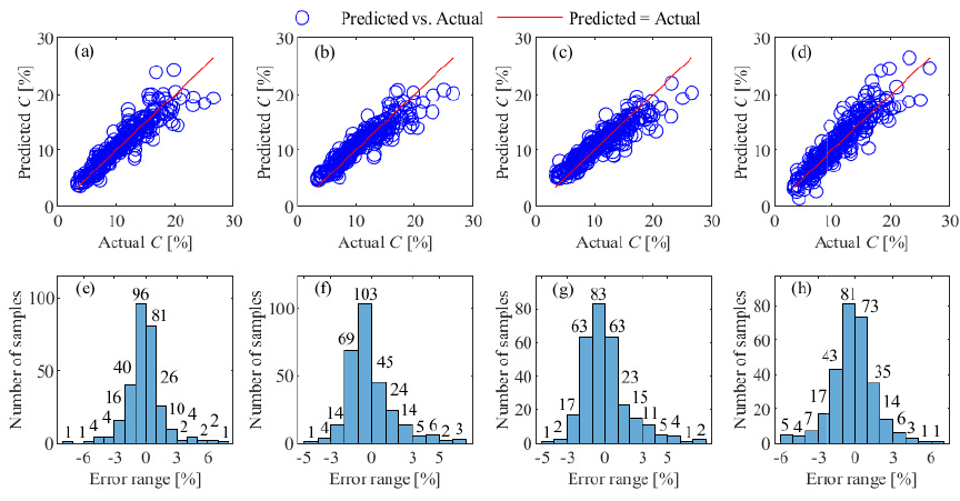
Fig. 8. CLR prediction results of different models on the testing data at \(L = 4\). (a)–(d) Prediction results of BO-XGBoost, BO-GBDT, BO-SVR, and BO-BPNN; (e)–(h) error distributions of BO-XGBoost, BO-GBDT, BO-SVR, and BO-BPNN.
Under the FCM-based four-cluster operating condition classification framework, the results (Table 2) show that none of the four comparative models achieved \(R^2\) values exceeding 0.86, RMSE below 0.0167, MAE lower than 1.14%, or MAPE under 10.47%. Comparative analysis with BO-RF demonstrates their inferior CLR prediction capability. While all models exhibited acceptable fitting accuracy with actual values, the BO-RF’s error distribution significantly outperformed others: 92.76% of BO-XGBoost and BO-GBDT predictions, 91.03% of BO-SVR, and 90.69% of BO-BPNN fell within the [\(-3\)%, 3%] error range. The results of quantitative analysis conclusively demonstrate that the prediction capability of the BO-RF is superior to that of the CLR, exhibiting statistically significant advantages over comparative models in stability and accuracy. The average training time for the presented BO-RF model is 18 minutes. Hyperparameter optimization dominates 85% of this time.
All experimental results (Figs. 5–8) reveal a clear and robust pattern: the most significant prediction errors systematically occur when the actual CLR is abnormally high, typically exceeding 20%. In the actual production process, the normal design range for CLR is between 9% and 15%. A sustained CLR above 20% clearly indicates a distressed or abnormal operating condition in the SAG mill, typically resulting from severe process disturbances such as a sudden, significant increase in ore hardness or a malfunction of the vibrating screen, which drastically reduce grinding efficiency. The model’s performance degradation in this regime is a classic manifestation of the extrapolation problem inherent to data-driven models. These high-CLR events are rare and were consequently under-represented in our training dataset. As visually evident in the data distribution, samples with CLR greater than 20% are far fewer. Therefore, the model lacked sufficient examples to learn the complex dynamics of these inefficient operational states and is less reliable when making predictions outside the core data distribution it was trained on.
5.5. Feature Importance Analysis
To enhance the industrial applicability of our high-accuracy CLR prediction model and provide actionable insights for operational decision-making, we conducted a Gini importance analysis to quantify feature influence on CLR predictions.
For a node \(t\) with \(Q\) classes, Gini impurity measures label distribution purity:
When splitting node \(t\) into child nodes \(t_L\) (left) and \(t_R\) (right) using feature \(f\), compute impurity reduction:
The importance of feature \(f\) in tree \(T_k\) is the sum of impurity reductions over all splits using \(f\):
Adjust for node sample size to prioritize high-impact splits:
Average normalized importance across all \(K\) trees:
Table 3. Gini importance analysis results.

Gini importance analysis results (Table 3) quantify the relative influence of input features on CLR prediction, revealing circulating load (\(F\)) as the dominant driver (87.63% importance). This dominance stems from its direct mechanistic link to CLR, where \(F\) defines the mass of recycled unground material. Mill power (\(W\)) and water flows (\(V_1\), \(V_2\), and \(V_3\)) exhibit secondary effects (3.0%–1.8% each), primarily modulating grinding efficiency through slurry viscosity and screening dynamics. Fresh ore feed rate (\(G\), 2.50%) contributes minimally due to its inverse relationship with \(F\). For plant operations, this implies \(F\)-sensing requires highest reliability, and water flows offer leverage for CLR stabilization. \(W\) monitoring can be relaxed outside abnormal operating conditions.
6. Conclusion
Grinding is a process of achieving ore size reduction, which plays a key role in subsequent mineral separation. Modeling and optimization of the grinding process has been a hot research topic in the field of mineral processing. In this paper, a hybrid framework integrating FCM and BO-RF is used to predict the CLR in an SAG process. Key process parameters affecting the CLR were identified by analyzing the operating mechanism of the SAG process. Based on mechanistic analysis, appropriate parameters were selected to perform operating condition clustering for the SAG process. Within each cluster, the BO-RF approach was adopted to model the CLR. Simulation results based on actual production data demonstrate that this method achieves over 90% accuracy in CLR prediction, with the prediction error maintained within 1.1%. Comparative experimental results validated the superior predictive capability of the presented method for CLR. The presented model is able to serve as a predictor, using historical data and future inputs to forecast CLR trends. It enables dynamic parameter adjustments for stabilization. Operators can verify production states and adjust SAG parameters in real time if predictions deviate. By explicitly addressing the inherent complexities of nonlinear dynamics, multiple operating conditions, and time-delay characteristics, the presented methodology not only enables accurate CLR prediction but also establishes a generalizable framework applicable to similar industrial processes requiring multivariate dynamic modeling.
However, validation is limited to one type of ore. Future work will extend this method to heterogeneous ores. Specifically, we will study \(L\)-optimization for mixed ores by integrating ore properties into FCM feature vectors. To further improve equipment adaptability, online learning mechanisms will be investigated to enable real-time model updates. Additionally, feature selection and model simplification strategies will be explored to reduce system complexity for practical deployment. In addition, a systematic framework for sensitivity and ablation analysis will also be developed to quantify the robustness of the model to industrial disturbances (such as non-Gaussian noise and multi-ore heterogeneity) and to isolate the contribution of its key components, thereby improving the deployment readiness of real-time control systems.
Acknowledgments
This work was supported in part by the Natural Science Foundation of Hubei Province, China, under Grant 2020CFA031; and JSPS (Japan Society for the Promotion of Science) KAKENHI under Grants 24K03325 and 25K07807.
- [1] K. B. Owusu, W. Skinner, and R. Asamoah, “Feed hardness and acoustic emissions of autogenous/semi-autogenous (AG/SAG) mills,” Miner. Eng., Vol.187, Article No.107781, 2022. https://doi.org/10.1016/j.mineng.2022.107781
- [2] Z.-X. Zhang, J. A. Sanchidrián, F. Ouchterlony, and S. Luukkanen, “Reduction of Fragment Size from Mining to Mineral Processing: A Review,” Rock Mechanics and Rock Engineering, Vol.56, No.1 pp. 747-778, 2023. https://doi.org/10.1007/s00603-022-03068-3
- [3] K. B. Owusu, M. Zanin, W. Skinner, and R. Asamoah, “AG/SAG mill acoustic emissions characterisation under different operating conditions,” Miner. Eng., Vol.171, Article No.107098, 2021. https://doi.org/10.1016/j.mineng.2021.107098
- [4] M. Fang, D. Zheng, X. Qiu, and Y. Du, “A Control System for the Ball Mill Grinding Process Based on Model Predictive Control and Equivalent-Input-Disturbance Approach,” J. Adv. Comput. Intell. Intell. Inform., Vol.20, No.7, pp. 1152-1158, 2016. https://doi.org/10.20965/jaciii.2016.p1152
- [5] A. Kumar, R. Sahu, and S. K. Tripathy, “Energy-Efficient Advanced Ultrafine Grinding of Particles Using Stirred Mills—A Review,” Energies, Vol.16, Issue 14, Article No.5277, 2023. https://doi.org/10.3390/en16145277
- [6] M. Hadizadeh, A. Farzanegan, and M. Noaparast, “A plant-scale validated MATLAB-based fuzzy expert system to control SAG mill circuits,” J. of Process Control, Vol.70, pp. 1-11, 2018. https://doi.org/10.1016/j.jprocont.2018.08.003
- [7] L. E. Olivier, M. G. Maritz, and I. K. Craig, “Estimating Ore Particle Size Distribution Using a Deep Convolutional Neural Network,” IFAC-PapersOnLine, Vol.53, Issue 2, pp. 12038-12043, 2020. https://doi.org/10.1016/j.ifacol.2020.12.740
- [8] J. Tang, J. Qiao, Z. Liu, X. Zhou, G. Yu, and J. Zhao, “Mechanism characteristic analysis and soft measuring method review for ball mill load based on mechanical vibration and acoustic signals in the grinding process,” Miner. Eng., Vol.128, pp. 294-311, 2018. https://doi.org/10.1016/j.mineng.2018.09.006
- [9] X. Fang, C. Wu, N. Liao, C. Yuan, B. Xie, and J. Tong, “The first attempt of applying ceramic balls in industrial tumbling mill: A case study,” Miner. Eng., Vol.180, Article No.107504, 2022. https://doi.org/10.1016/j.mineng.2022.107504
- [10] H. Wei, Y. He, S. Wang, W. Xie, W. Zuo, and F. Shi, “Effects of circulating load and grinding feed on the grinding kinetics of cement clinker in an industrial CKP mill,” Powder Technology, Vol.253, pp. 193-197, 2014. https://doi.org/10.1016/j.powtec.2013.11.016
- [11] H. Dündar, “Investigating the benefits of replacing hydrocyclones with high-frequency fine screens in closed grinding circuit by simulation,” Miner. Eng., Vol.148, Article No.106212, 2020. https://doi.org/10.1016/j.mineng.2020.106212
- [12] N. Li, L. Li, J. Wang, Z. Liu, Q. Feng, Q. Zhang, H. Liu, B. Klein, and B. Li, “Prediction of Circulation Load of Side-Flanged High-Pressure Grinding Rolls Closed-Circuit Crushing,” Minerals, Vol.15, Issue 6, Article No.603, 2025. https://doi.org/10.3390/min15060603
- [13] T. Chai, L. Zhai, and H. Yue, “Multiple models and neural networks based decoupling control of ball mill coal-pulverizing systems,” J. of Process Control, Vol.21, Issue 3, pp. 351-366, 2011. https://doi.org/10.1016/j.jprocont.2010.11.007
- [14] J. D. le Roux, A. Steinboeck, A. Kugi, and I. K. Craig, “Steady-state and dynamic simulation of a grinding mill using grind curves,” Miner. Eng., Vol.152, Article No.106208, 2020. https://doi.org/10.1016/j.mineng.2020.106208
- [15] J. T. McCoy and L. Auret, “Machine learning applications in minerals processing: A review,” Miner. Eng., Vol.132, pp. 95-109, 2019. https://doi.org/10.1016/j.mineng.2018.12.004
- [16] Z. Liao, C. Xu, W. Chen, F. Wang, and J. She, “Multi-model integration for predicting circulating load ratio based on clustering SAG milling operating conditions,” Control Eng. Pract., Vol.153, Article No.106129, 2024. https://doi.org/10.1016/j.conengprac.2024.106129
- [17] J. Hu, M. Wu, L. Chen, K. Zhou, P. Zhang, and W. Pedrycz, “Weighted Kernel Fuzzy C-Means-Based Broad Learning Model for Time-Series Prediction of Carbon Efficiency in Iron Ore Sintering Process,” IEEE Trans. on Cybernetics, Vol.52, Issue 6, pp. 4751-4763, 2022. https://doi.org/10.1109/TCYB.2020.3035800
- [18] L. Lin, S. Li, K. Wang, B. Guo, H. Yang, W. Zhong, P. Liao, and P. Wang, “A new FCM-XGBoost system for predicting Pavement Condition Index,” Expert Syst. Appl., Vol.249, Part B, Article No.123696, 2024. https://doi.org/10.1016/j.eswa.2024.123696
- [19] F. Hassanpour, S. Sharifazari, K. Ahmadaali, S. Mohammadi, and Z. Sheikhalipour, “Development of the FCM-SVR Hybrid Model for Estimating the Suspended Sediment Load,” KSCE J. Civ. Eng., Vol.23, Issue 6, pp. 2514-2523, 2019. https://doi.org/10.1007/s12205-019-1693-7
- [20] D. Graves and W. Pedrycz, “Kernel-based fuzzy clustering and fuzzy clustering: A comparative experimental study,” Fuzzy Sets Syst., Vol.161, Issue 4, pp. 522-543, 2010. https://doi.org/10.1016/j.fss.2009.10.021
- [21] J. Fan and J. Wang, “A Two-Phase Fuzzy Clustering Algorithm Based on Neurodynamic Optimization with Its Application for PolSAR Image Segmentation,” IEEE Trans. Fuzzy Syst., Vol.26, Issue 1, pp. 72-83, 2018. https://doi.org/10.1109/TFUZZ.2016.2637373
- [22] B. Chen, J. Hu, L. Duan, and Y. Gu, “Network Administrator Assistance System Based on Fuzzy C-means Analysis,” J. Adv. Comput. Intell. Intell. Inform., Vol.13, No.2, pp. 91-96, 2009. https://doi.org/10.20965/jaciii.2009.p0091
- [23] L. Breiman, “Random Forests,” Mach. Learn., Vol.45, pp. 5-32, 2001. https://doi.org/10.1023/A:1010933404324
- [24] M. S. H. Lipu, M. A. Hannan, A. Hussain, S. Ansari, S. A. Rahman, and M. H. M. Saad, “Real-Time State of Charge Estimation of Lithium-Ion Batteries Using Optimized Random Forest Regression Algorithm,” IEEE Trans. Intell. Veh., Vol.8, Issue 1, pp. 639-648, 2022. https://doi.org/10.1109/TIV.2022.3161301
- [25] M. G. Alfarizi, B. Tajiani, J. Vatn, and S. Yin, “Optimized Random Forest Model for Remaining Useful Life Prediction of Experimental Bearings,” IEEE Trans. Ind. Inf., Vol.19, No.6, pp. 7771-7779, 2023. https://doi.org/10.1109/TII.2022.3206339
- [26] J. Olivier and C. Aldrich, “Use of Decision Trees for the Development of Decision Support Systems for the Control of Grinding Circuits,” Minerals, Vol.11, Issue 6, Article No.595, 2021. https://doi.org/10.3390/min11060595
- [27] C. Loudari, M. Cherkaoui, R. Bennani, I. El Harraki, O. Fares, and M. El Adnani, “Predicting Grinding Mill Power Consumption in Mining: A Comparative Study,” 2023 7th IEEE Congress on Information Science and Technology (CiSt), pp. 395-399, 2023. https://doi.org/10.1109/CiSt56084.2023.10410011
- [28] L. F. Napier and C. Aldrich, “An IsaMill™ Soft Sensor based on Random Forests and Principal Component Analysis,” IFAC-PapersOnLine, Vol.50, Issue 1, pp. 1175-1180, 2017. https://doi.org/10.1016/j.ifacol.2017.08.270
- [29] R. K. Inapakurthi, S. S. Miriyala, and K. Mitra, “Recurrent neural networks based modelling of industrial grinding operation,” Chem. Eng. Sci., Vol.219, Article No.115585, 2020. https://doi.org/10.1016/j.ces.2020.115585
- [30] Z. Ghasemi, F. Neumann, M. Zanin, J. Karageorgos, and L. Chen, “A comparative study of prediction methods for semi-autogenous grinding mill throughput,” Miner. Eng., Vol.205, Article No.108458, 2024. https://doi.org/10.1016/j.mineng.2023.108458
- [31] A. M. Elshewey, M. Y. Shams, N. El-Rashidy, A. M. Elhady, S. M. Shohie, and Z. Tarek, “Bayesian Optimization with Support Vector Machine Model for Parkinson Disease Classification,” Sensors, Vol.23, Issue 4, Article No.2085, 2023. https://doi.org/10.3390/s23042085
- [32] D. Maclaurin, D. Duvenaud, and R. P. Adams, “Gradient-based hyperparameter optimization through reversible learning,” Proc. of the 32nd Int. Conf. on Machine Learning, Vol.37, pp. 2113-2122, 2015.
- [33] M. Aghaabbasi, M. Ali, M. Jasiński, Z. Leonowicz, and T. Novák, “On Hyperparameter Optimization of Machine Learning Methods Using a Bayesian Optimization Algorithm to Predict Work Travel Mode Choice,” IEEE Access, Vol.11, pp. 19762-19774, 2023. https://doi.org/10.1109/ACCESS.2023.3247448
- [34] T. Shaqarin and B. R. Noack, “A Fast-Converging Particle Swarm Optimization through Targeted, Position-Mutated, Elitism (PSO-TPME),” Int. J. Comput. Intell. Syst., Vol.16, No.1, Article No.6, 2023. https://doi.org/10.1007/s44196-023-00183-z
- [35] E. C. Garrido-Merchán and D. Hernández-Lobato, “Dealing with categorical and integer-valued variables in Bayesian optimization with Gaussian processes,” Neurocomputing, Vol.380, pp. 20-35, 2020. https://doi.org/10.1016/j.neucom.2019.11.004
- [36] H. Cho, Y. Kim, E. Lee, D. Choi, Y. Lee, and W. Rhee, “Basic Enhancement Strategies When Using Bayesian Optimization for Hyperparameter Tuning of Deep Neural Networks,” IEEE Access, Vol.8, pp. 52588-52608, 2020. https://doi.org/10.1109/ACCESS.2020.2981072
- [37] J. Zhan, X. Huang, Y. Qian, and W. Ding, “A Fuzzy C-Means Clustering-Based Hybrid Multivariate Time Series Prediction Framework with Feature Selection,” IEEE Trans. Fuzzy Syst., Vol.32, Issue 8, pp. 4270-4284, 2024. https://doi.org/10.1109/TFUZZ.2024.3393622
- [38] J. C. Bezdek, R. Ehrlich, and W. Full, “FCM: The fuzzy c-means clustering algorithm,” Comput. Geosci., Vol.10, Issues 2-3, pp. 191-203, 1984. https://doi.org/10.1016/0098-3004(84)90020-7
- [39] G. Yan, Q. Sun, J. Huang, and Y. Chen, “Helmet Detection Based on Deep Learning and Random Forest on UAV for Power Construction Safety,” J. Adv. Comput. Intell. Intell. Inform., Vol.25, No.1, pp. 40-49, 2021. https://doi.org/10.20965/jaciii.2021.p0040
This article is published under a Creative Commons Attribution-NoDerivatives 4.0 Internationa License.