Research Paper:
Polytomous Model Integrating S–P Chart and Ordering Theory: Application to Cognitive Diagnosis of Fraction Calculation

This study proposes an integrated model for cognition diagnosis applicable to polytomous data and conducts an empirical analysis using data on fraction addition and subtraction performance collected from elementary school students in Taiwan and Japan. This study develops computational procedures that extend the dichotomous student–problem (S–P) chart and ordering theory (OT) to polytomous response formats. The integrated polytomous student problem–ordering theory (SP–OT) model consists of a three-step procedure: (1) calculation of the caution indices of test-takers based on the polytomous S–P chart; (2) implementation of a two-stage cluster analysis using both the caution indices and score as clustering indicators; (3) construction of polytomous OT item structures for each cluster derived from the two-stage cluster analysis. The polytomous SP–OT model captured varying levels of student understanding and provided richer diagnostic insights. Furthermore, this model enhanced the accuracy and effectiveness of educational assessment. This study provided valuable methodological insights by developing a polytomous model that integrated the S–P chart and OT. This new model overcame the limitations of traditional dichotomous data by introducing a visualized and clustered approach to cognitive diagnosis. Future research may apply this polytomous SP–OT model to other disciplines.
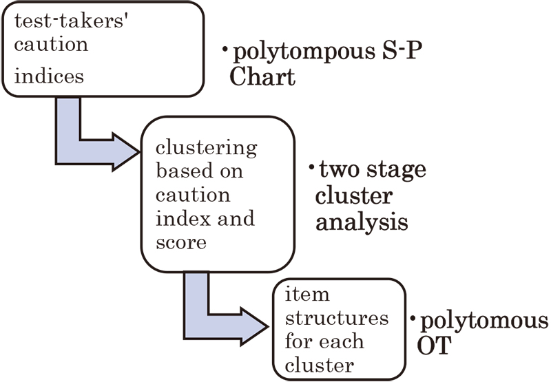
Procedure of the integrated polytomous SP―OT model for conducting cognitive diagnosis
1. Introduction
The student–problem chart (S–P chart) and ordering theory (OT) can be used for cognitive diagnoses 1,2,3. However, the traditional S–P chart and OT have scoring limitations in that they can be applied only to dichotomous scoring data, making them unsuitable for the more commonly encountered polytomous data in cognitive diagnoses. Therefore, the first purpose of this study is to improve the scoring limitations of the S–P chart and OT by developing S–P chart and OT models applicable to polytomous data. Additionally, the S–P chart is a data-oriented cognitive diagnosis method whose main benefit lies in calculating the caution index of each test-taker and clustering test-takers into groups, with each group reflecting its characteristics of concepts and knowledge. However, OT is a graphical-oriented cognitive diagnosis method that analyzes graphical item structures and linkages based on the item response patterns of test-takers and reveals the characteristics of concepts and knowledge.
If the advantages of these two cognitive diagnosis methodologies could be integrated to provide cognitive diagnosis information that is both data-driven and graphical, they would significantly contribute to cognitive diagnosis methodologies. Therefore, the second purpose of this study is to integrate the polytomous S–P chart and polytomous OT and conduct a polytomous cognitive diagnosis of fraction addition and subtraction data collected from elementary school students in Taiwan and Japan.
2. Literature Review
2.1. Cognitive Diagnosis and its Utilities
Cognitive diagnosis is a psychological assessment paradigm that extends beyond traditional testing by providing fine-grained information on the mastery of specific cognitive attributes by learners. Its primary significance lies in enabling educators and researchers to identify the cognitive strengths and weaknesses of individuals. Cognitive diagnosis helps identify misconceptions and better understand the underlying processes that lead to correct or incorrect responses. Cognitive diagnosis relies on cognitive theory with psychometric modeling 4. Cognitive diagnosis, such as the deterministic inputs noisy “and” gate (DINA) and generalized DINA (G-DINA) models, analyze the relationship between test items and required cognitive attributes. By analyzing the response patterns across items, cognitive diagnosis estimates the mastery probabilities of learners for each attribute. Recent advancements have extended cognitive diagnosis to polytomous data and integrated it with visual or graphical methods, broadening its applicability across educational contexts.
Future directions for cognitive diagnosis methods include integrating multilevel models and longitudinal data analyses to track dynamic changes in the conceptual understanding of students. Additionally, developing models that handle polytomous data can overcome the limitations of dichotomous scoring. Incorporating artificial intelligence and natural language processing for automated diagnosis and item generation will further expand the applicability of cognitive diagnosis, enabling more timely and personalized learning assessment and support 5.
The S–P chart and OT are two branches of cognitive diagnosis. They can visualize item hierarchies and classify learners into cognitive profiles based on the response consistency. The value of cognitive diagnosis lies in its capacity to inform tailored instruction and remediation, design targeted interventions, and support the development of adaptive learning systems. Furthermore, cognitive diagnosis provides empirical evidence for validating curriculum structures and enhances the alignment between assessments and cognitive learning objectives, ultimately contributing to more effective learner-centered educational practices 6,7.
Polytomous cognitive diagnosis plays a crucial role in accurately assessing the varying degrees of understanding by students, rather than relying on binary right or wrong judgments. This reveals a continuum of learning progression and conceptual mastery across multiple levels. Therefore, developing a polytomous S–P chart is essential because it visualizes the performance patterns of students, highlights key learning obstacles, and assists teachers in providing precise evidence-based instructional guidance to enhance conceptual understanding and learning effectiveness 7.
2.2. Dichotomous S–P Chart and Ordering Theory
The dichotomous S–P chart was proposed by Sato in the 1980s. The dichotomous S–P method primarily analyzes the response patterns of test-takers in assessments to help teachers diagnose the learning profiles of test-takers and evaluate the quality of the test items. This analysis serves as a reference for implementing remedial instructions and improving the test design. The response patterns of test-takers not only reflect their test scores but also indicate their understanding of the concepts assessed by the items. Consequently, test-takers with the same total scores but different response patterns may exhibit different levels of conceptual understanding. Therefore, total scores alone cannot accurately capture the conceptual knowledge of test-takers. Instead, analyzing response patterns provides insight into the learning processes of students and helps identify potential flaws in test items 8.
The dichotomous S–P chart model is described as follows: Suppose a test consists of \(N\) (\(i=1,2,\dots,N)\) test-takers and \(M\) (\(j=1,2,\dots,M)\) dichotomously scored items. The response data can be represented as a data matrix \(Y=(y_{ij})_{N\times M}\), where \(y_{ij}=1\) indicates that test-taker \(i\) answers item \(j\) correctly, and \(y_{ij}=0\) indicates an incorrect response on item \(j\). The S–P chart provides caution index \(\textit{CS}_i\) for each test-taker \(i\) defined as follows 9:
Table 1. Contingency table for dichotomous items \(i\) and \(j\).

The OT is used to analyze the ordering relationships among items based on the response data of test-takers, thereby revealing the knowledge structure of test-takers. The OT focuses on dichotomously scoring items and uses contingency table data to calculate the prerequisites or ordering relationships between items 10. For instance, given two dichotomous items \(i\) and \(j\), the contingency table of the number of test-takers answering each combination of correct (coded as 1) and incorrect (coded as 0) responses is presented in Table 1.
The data in Table 1 define a directional measure to quantify whether item \(i\) is a prerequisite for item \(j\). Coefficient \(n_{01}/n\) ranges from 0 to 1, with smaller values indicating a higher likelihood that item \(i\) serves as a prerequisite for item \(j\). Threshold \(\varepsilon\) (\(0<\varepsilon<1\)) determines whether a prerequisite relationship exists between items.
-
If \((n_{01}/n)<\varepsilon\), it indicates that item \(i\) is a prerequisite for item \(j\), indicating an ordering relationship. This is represented as \(i\to j\) in the graphical knowledge structure.
-
If \((n_{01}/n)\ge \varepsilon\), it indicates that item \(i\) is not a prerequisite for item \(j\), and thus no ordering relationship exists. This is represented graphically without a directional arrow.
The OT is an important framework for exploring hierarchical relationships among test items and identifying the sequential structure of the knowledge acquisition by students. This helps to reveal the manner in which the mastery of one concept supports the understanding of subsequent concepts. Developing a polytomous OT further extends this framework by capturing partial mastery levels rather than simple binary outcomes. This advancement allows for a more nuanced interpretation of learning progress, supports the design of adaptive instruction, and provides a deeper understanding of the cognitive development of students across different proficiency stages 10.
2.3. Fraction Concept of Students and Calculation
Understanding fractions is a critical component of elementary mathematics education because it lays the foundation for the success of students in advanced mathematical topics such as ratios, proportions, algebra, and probability. In elementary school curricula, students typically encounter several key types of fractions that form the basis of their fraction knowledge. First, they learn unit fractions that represent quantities with a numerator of one (for example, \(1/2\) and \(1/4\)) and are essential for building an understanding of the partitioning of wholes into equal parts. Subsequently, they progress to proper fractions in which the numerator is smaller than the denominator, reflecting parts less than a whole 11. Students also engage with improper fractions and mixed numbers that extend their understanding to quantities greater than one whole, as seen in examples such as \(5/4\) or \(1(1/2)\). In certain curricula, equivalent fractions are introduced early to help students grasp that different-looking fractions can represent the same value (for example, \(2/4=1/2\)). Moreover, benchmark fractions such as \(1/2\), \(1/4\), and \(3/4\) are emphasized to support the estimation and comparison skills. These fraction types are often taught through visual models—such as area models, set models, and number lines—that facilitate the conceptual development of students. Mastery of these fraction types improves the computational abilities of students and prepares them for advanced concepts in proportional reasoning and rational number operations.
Fraction knowledge enables students to develop a deeper sense of numbers and operations beyond whole numbers, supporting flexible thinking and problem solving. Conceptually, fraction understanding can be categorized into part–whole, measure, quotient, ratio, and operator interpretations. The part–whole concept emphasizes fractions as parts of a single whole, whereas the measure concept views fractions as quantities representing distance or magnitude on a number line. The quotient perspective connects fractions to division, highlighting the manner in which fractions can represent the outcome of dividing two whole numbers. The ratio concept frames fractions as comparisons between two quantities that are essential for proportional reasoning. Finally, the operator view considers fractions as transformations that scale quantities. Despite the importance of these conceptual types, students often develop persistent misconceptions about fractions 12. Common fraction misconceptions include overgeneralizing whole number knowledge. For instance, students may believe that \(1/8\) is larger than \(1/4\) because 8 is greater than 4, or they interpret numerators and denominators in isolation without understanding their relational meaning 13,14. Additionally, students may assume that larger denominators always produce larger fractions or misunderstand equivalent fractions, thus failing to recognize their identical values. Addressing these misconceptions requires targeted instructional interventions that emphasize conceptual understanding, visual representations, and meaningful practices. Therefore, cultivating a robust and flexible grasp of fraction concepts during elementary education is essential to prevent long-term difficulties in mathematics learning and to support the progression of students to higher-level mathematical thinking 15,16.
When performing fraction addition and subtraction, elementary students frequently exhibit misconceptions rooted in their incomplete understanding of fraction operations. A prevalent error is the “add across” misconception, where students add the numerators and denominators separately (for example, \(1/2+1/4=2/6\)), reflecting an overgeneralization of whole number addition rules. Another common misconception is ignoring the need for common denominators, leading students to incorrectly combine fractions with unlike denominators without finding equivalent fractions. Additionally, certain students incorrectly believe that adding fractions always results in a larger quantity, even when adding two fractions that together sum to less than one whole (for example, \(1/8+1/8=2/16\) interpreted as greater than \(1/8\)). Students may also confuse numerators and denominators, assuming that a larger denominator produces a larger sum or that subtracting a smaller fraction from a larger one always yields a smaller fraction without considering the actual values. Addressing these misconceptions requires explicit instruction, hands-on activities with visual models, and opportunities for students to explain their reasoning 17,18.
3. Research Design
Because the dichotomous S–P chart and OT are only applicable to dichotomous data and cognitive diagnosis data are often polytomous, this study first extends both the S–P chart and OT to accommodate polytomous data. Subsequently, it integrates the S–P chart and OT models and applies them to the analysis of polytomous fraction addition and subtraction items.
This study applied an integrated polytomous SP–OT model to analyze the performance of elementary school students on 11 fraction addition and subtraction items. These included fraction calculations using the same denominator, fractions with different denominators, and mixed fractions. In total, 843 elementary school students participated in this study, comprising 435 students from Taiwan and 408 from Japan. Based on the responses of the 843 students, data analysis was conducted using the three-step procedure of the integrated polytomous SP–OT model.
3.1. Computation of Polytomous S–P Chart
The computational steps of the polytomous S–P chart are as follows:
-
Step 1:
For each test-taker \(n\) (\(n=1,2,\dots,N)\), the polytomous scoring data across all items are represented as a response pattern vector \(Y'_n=(y'_{n1},y'_{n2},\dots,y'_{nM})=(y'_{nm})_{1\times M}\), where the full score for item \(m\) (\(m=1,2,\dots,M)\) is defined as \(K_m\). The response data matrix for all test-takers is given can be expressed as follows:
\begin{equation} \label{eq:2} \boldsymbol{Y}'=\left(y'_{nm}\right)_{N\times M}= \begin{bmatrix} Y'_1\\ \vdots \\ Y'_N\\ \end{bmatrix}. \end{equation} -
Step 2:
Matrix \(\boldsymbol{Y}'\) is standardized to obtain standardized response data matrix \(\boldsymbol{SY}'=(sy'_{\textit{nm}})_{N\times M}\), where \(sy'_{\textit{nm}}=y'_{\textit{nm}}/K_m\) with \(0\le sy'_{\textit{nm}}\le 1\). The sum of standardized scores for test-taker \(n\) across all items is denoted as \(sy'_{n\bullet}=\sum_{m=1}^M sy'_{\textit{nm}}\), and the sum of standardized scores for item \(m\) across all test-takers is denoted as \(sy'_{\bullet m}=\sum_{n=1}^N sy'_{\textit{nm}}\).
-
Step 3:
Test-takers with higher \(sy'_{n\bullet}\) values are considered to perform better, and items with higher \(sy'_{\bullet m}\) values are regarded as easier items. The rows of standardized response data matrix \(\boldsymbol{SY}'\) are sorted in descending order of \(sy'_{n\bullet}\), and the columns are sorted in descending order of \(sy'_{\bullet m}\), resulting in sorting matrix \(SY=(sy_{\textit{nm}})_{N\times M}\) of the S–P chart.
-
Step 4:
Let \({sy}_{n\bullet}=\sum_{m=1}^M sy_{\textit{nm}}\) and \(sy_{\bullet m}=\sum_{n=1}^N sy_{\textit{nm}}\), where \(M\ge sy_{1\bullet}\ge sy_{2\bullet}\ge\cdots\ge sy_{N\bullet}\ge 0\) and \(N\ge sy_{\bullet 1}\ge sy_{\bullet 2}\ge \cdots \ge sy_{\bullet M}\ge 0\).
-
Step 5:
Define the perfect response matrix. \(\boldsymbol{SY}_{\boldsymbol{n}}^{\,\boldsymbol{PC}}=(sy_{\textit{nm}}^{\,\textit{pc}})_{N\times M}\), where \([\,\cdot\,]\) is Gauss symbol and \(e_{\textit{nm}}=sy'_{n\bullet}-[sy'_{n\bullet}]\). It is
\begin{equation} \label{eq:3} {sy}_{\textit{nm}}^{\,\textit{pc}}= \begin{cases} 1, & 1\le m\le \left[sy'_{n\bullet}\right],\\ e_{\textit{nm}}, & m=\left[sy'_{n\bullet}\right]+1,\\ 0, & \mbox{else}.\\ \end{cases} \end{equation} -
Step 6:
The discrepancy between the actual and perfect response patterns of a test-taker is used to calculate the caution index of the test-taker. Specifically, caution index \({\textit{CI}}_n\) for test-taker \(n\) is defined as follows:
\begin{equation} \label{eq:4} \textit{CI}_n=\sqrt{\dfrac{1}{M}\sum_{m=1}^M \left(sy_{\textit{nm}}-sy_{\textit{nm}}^{\,\textit{pc}}\right)^2}\,. \end{equation}\({\textit{CI}}_n\) quantifies the degree of inconsistency between the observed and perfect response patterns.
Table 2. Example of response data matrix.

Table 3. Standardized response data matrix.

An illustrative example of the calculation is as follows:
For Step 1, let the number of test-takers be \(N=10\), number of items be \(M=6\), and the full score for items is \(K_1=3\), \(K_2=3\), \(K_3=2\), \(K_4=2\), \(K_5=2\), \(K_6=1\). Response data matrix \(\boldsymbol{Y}'=(y'_{\textit{nm}})_{N\times M}\) for all the test-takers is presented in Table 2.
For Step 2, standardized response data matrix \(\boldsymbol{SY}'=(sy'_{\textit{nm}})_{N\times M}\) is presented in Table 3.
For Steps 3 and 4, sorting matrix \(\textit{SY}=({sy}_{\textit{nm}})_{N\times M}\) is presented in Table 4.
For Step 5, perfect response matrix \(\boldsymbol{SY}_{\boldsymbol{n}}^{\,\boldsymbol{PC}}=(sy_{\textit{nm}}^{\,\textit{pc}})_{N\times M}\) is presented in Table 5.
For Step 6, caution indices \(\textit{CI}_n\) for all test-takers are listed in Table 6.
Table 4. Sorting matrix of standardized response data matrix.

Table 5. Perfect response matrix.

Table 6. Caution indices for all test-takers.

3.2. Computation of Polytomous Ordering Theory
The computational steps for the polytomous OT are as follows. According to the computations of the polytomous OT, the dichotomous OT can be regarded as a special case of the polytomous OT.
-
Step 1:
Suppose that item \(i\) and item \(j\) have scoring points of \(C_i\) and \(C_j\), respectively, denoted as \(k=0,1,\dots,(C_i-1)\) and \(l=0,1,\dots,(C_j-1)\), respectively. The total number of test-takers is represented as \(n=\sum_{k=0}^{C_i-1} \sum_{l=0}^{C_j-1} n_{\textit{kl}}\), as presented in Table 7.
-
Step 2:
Using normalization, the number of frequencies that the prerequisite relationship “item \(i\) \(\to\) item \(j\)” is not satisfied can be calculated as follows:
\begin{equation} \label{eq:5} n'=\sum_k \sum_l n_{\textit{kl}},\quad \forall\ \dfrac{k+1}{C_i}<\frac{l+1}{C_j}. \end{equation} -
Step 3:
A directional coefficient \(n'/n\) is defined to measure whether item \(i\) serves as a prerequisite for item \(j\). Coefficient \(n'/n\) ranges from zero to one, with smaller values indicating a greater likelihood that item \(i\) is a prerequisite for item \(j\).
-
Step 4:
Based on threshold \(\varepsilon\) (\(0<\varepsilon<1\)), the ordering relationship between items is determined as follows:
-
If \((n'/n)<\varepsilon\), item \(i\) is considered a prerequisite for item \(j\), indicating an ordering relationship represented as \(i\to j\) in a graphical knowledge structure.
-
If \((n'/n)\ge \varepsilon\), item \(i\) is not a prerequisite for item \(j\), indicating the absence of an ordering relationship, and no arrow is drawn in the graphical representation.
-
Table 7. Contingency table for polytomous items \(i\) and \(j\).

Table 8. Directional coefficient \(n'/n\) matrix.

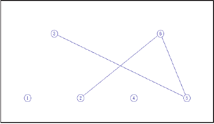
Fig. 1. Item structures of 10 test-takers.
An illustrative example of this calculation is provided below. Based on the response pattern matrix of 10 test-takers, directional coefficient \(n'/n\) matrix and item structures under threshold \(\varepsilon=0.1\) are presented in Table 8 and Fig. 1, respectively.
This study integrates the polytomous S–P chart and OT. This model is called the polytomous SP–OT model. The three-step procedure for conducting cognitive diagnosis was as follows: (1) calculation of the caution indices of the test-takers based on the polytomous S–P chart; (2) implementation of a two-stage cluster analysis using both the caution indices and score as clustering indicators; (3) construction of polytomous OT item structures for each cluster derived from the two-stage cluster analysis. This is shown in Fig. 2.
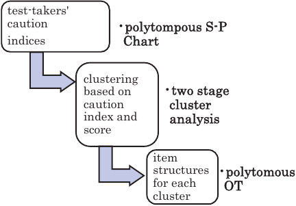
Fig. 2. Procedure of the integrated polytomous SP–OT model for conducting cognitive diagnosis.
3.3. Instrument of Fraction Calculation
The assessment instrument includes 11 fraction addition and subtraction items, each corresponding to a specific concept, as listed in Table 9. The scoring follows a polytomous scoring scheme: 2, 1, and 0. Here, 2 indicates a completely correct procedure and result, 1 indicates a partially correct response, and 0 indicates a completely incorrect response. Therefore, the maximum score of assessment is 22.
As presented in Table 10, item difficulty is represented by the score percentage, and item discrimination is determined using the Pearson correlation coefficient between each item and the total score. All Pearson correlation coefficients show statistically significant differences, indicating that item discrimination is acceptable.
Table 9. Fraction addition and subtraction items and concepts.

Table 10. Item difficulty and item discrimination.

3.4. Participants of Test-Takers
The test-takers in this study were sixth-grade elementary school students, including 435 students from Taiwan and 408 students from Japan. All these students had already learned the concept of fraction addition and subtraction in their mathematics courses. During the test development process, the researcher invited two elementary school teachers and one mathematics education professor to review the test items. Two elementary school teachers independently scored the responses of students. The Pearson correlation coefficient between the two sets of scores was 0.82 (\(p <.001\)), indicating a significant correlation and demonstrating inter-rater reliability.
4. Results and Discussions
This study applied an integrated polytomous SP–OT model to analyze the cognitive diagnostic performance of 843 sixth-grade elementary school students on 11 fraction addition and subtraction items. Data analysis was conducted according to the procedure of the integrated polytomous SP–OT model, as shown in Fig. 1.
4.1. Analysis of Caution Indices Based on the Polytomous S–P Chart
For the 843 test-takers in this study, the mean score was 17.6895 with a standard deviation of 6.4635. The mean caution index was 0.1752, with a standard deviation of 0.2193. The means and standard deviations for each item are listed in Table 11.
Table 11. Means and standard deviations of each item.

4.2. Results of Two-Stage Cluster Based on Caution Index and Score
This study conducted a two-stage cluster analysis using caution indices and scores. The optimal number of clusters was determined by minimizing the Akaike information criterion (AIC) and Bayesian information criterion (BIC). In this study, the number of clusters ranged from 2 to 10, and the optimal number of clusters was determined based on the AIC and BIC. As indicated in Table 12, both the AIC and BIC reached their lowest values when the number of clusters was seven. The analysis revealed that the optimal number of clusters was seven.
As presented in Table 13, Cluster I was characterized by a low caution index and low score. Cluster II had the largest number of test-takers and had a low caution index and an extremely high score. Cluster III demonstrated a high caution index but a moderate score. Cluster IV exhibited both a high caution index and high score. Cluster V was characterized by a low caution index and a moderate score. Cluster VI showed a low caution index and high score. Cluster VII had the second largest number of test-takers and demonstrated a high caution index and high score. Therefore, the characteristics of the cognitive diagnosis vary distinctly across clusters.
Table 12. Model selection based on AIC and BIC.

Table 13. Number of test-takers and mean of caution index and score in each cluster.

4.3. Item Structures of Each Cluster
This study set the threshold at \(\varepsilon=0.05\) to construct the item structures for each cluster of test-takers. Figs. 3–9 present the item structures for each cluster, illustrating the concept hierarchies and linkages of the items as perceived by the test-takers in each cluster.
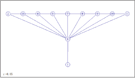
Fig. 3. Item structures of Cluster I.
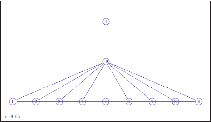
Fig. 4. Item structures of Cluster II.
Fig. 5. Item structures of Cluster III.
Fig. 6. Item structures of Cluster IV.
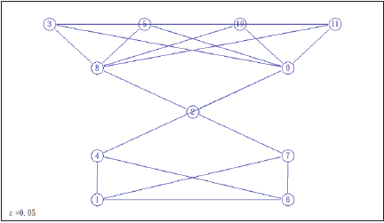
Fig. 7. Item structures of Cluster V.
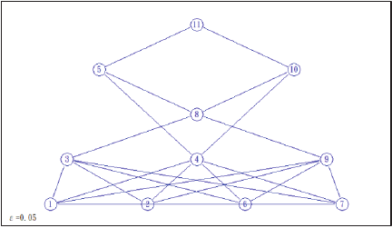
Fig. 8. Item structures of Cluster VI.
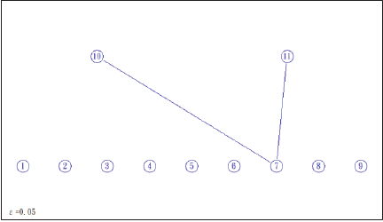
Fig. 9. Item structures of Cluster VII.
Figure 3 shows the item structures of Cluster I test-takers, revealing that the concept hierarchies consisted of three levels: Level 1 included item 1; Level 2 included item 6; Level 3 comprised items 2, 3, 4, 5, 7, 8, 9, 10, and 11. Cluster I test-takers were characterized by low caution indices and low scores. Therefore, remedial instructions had to begin by reinforcing the concepts of Level 1 items before progressing to the concepts in Levels 2 and 3. Test-takers in Cluster I could build on the mastery foundation established through item 1. By reviewing the concepts and calculations in item 6, they could enhance their mastery of all Level 3 items.
Figure 4 shows the item structures of Cluster II test-takers, indicating that the concept hierarchies had three levels: Level 1 included items 1, 2, 3, 4, 5, 6, 7, 8, and 9; Level 2 included item 10; Level 3 included item 11. Cluster II test-takers were characterized by low caution indices and extremely high scores, with their concept structures closely resembling those of the experts. For test-takers in Cluster II, reviewing item 10 from Level 2 could facilitate mastery of item 11 at Level 3.
Figure 5 presents the item structures of Cluster III test-takers, showing that the concept hierarchies consisted of four levels: Level 1 included items 1, 2, 3, 4, 6, and 7; Level 2 included items 5 and 9; Level 3 included items 8 and 11; Level 4 included item 10. Cluster III test-takers were characterized by high caution indices but moderate scores. Therefore, remedial instructions had to begin by reinforcing the concepts of Level 1 items, followed by sequential instruction on the concepts of Levels 2, 3, and 4. For example, the instruction could focus on strengthening the concept linkage among items 2 to 5.
Figure 6 illustrates the item structures of Cluster IV test-takers, showing that the concept hierarchy had only one level with no linkages between the items, indicating an isolated structure. Cluster IV test-takers were characterized by high caution indices and high scores. Although their scores were high, the lack of linkages between the items indicated that these test-takers might have answered randomly or possessed only procedural knowledge. Therefore, they had to develop a deeper understanding of the concepts underlying fraction addition and subtraction. For example, teachers could guide students to review and understand the differences and relationships between items 1 and 2.
Figure 7 displays the item structures of Cluster V test-takers, indicating that the concept hierarchies consisted of five levels: Level 1 included items 1 and 6; Level 2 included items 4 and 7; Level 3 included item 2; Level 4 included items 8 and 9; and Level 5 included items 3, 5, 10, and 11. Cluster V test-takers were characterized by low caution indices and moderate scores. Therefore, remedial instructions had to begin by reinforcing the concepts of Level 1 items, followed by sequential instruction on the concepts of Levels 2, 3, 4, and 5. For example, item 2 at Level 3 served as an essential conceptual bridge, representing the concept of “addition of fractions with unlike denominators that are multiples of each other.” Teachers could use this key concept to help test-takers comprehend the concepts and calculations involved in the Levels 4 and 5 items.
Figure 8 presents the item structures of Cluster VI test-takers, indicating that the concept hierarchies consisted of five levels: Level 1 included items 1, 2, 6, and 7; Level 2 included items 3, 4, and 9; Level 3 included item 8; Level 4 included items 5 and 10; and Level 5 included item 11. Cluster VI test-takers were characterized by low caution indices and high scores, showing similarities to Cluster II test-takers. Therefore, remedial instructions had to begin by reinforcing the concepts of Level 1 items, followed by sequential instruction on the concepts of Levels 2, 3, 4, and 5. For example, item 8 at Level 3 was a critical conceptual bridge that involved the “subtraction of fractions with unlike denominators that are not multiples of each other.” Teachers could use this core concept to assist test-takers in understanding the concepts and computations of the Levels 4 and 5 items.
Figure 9 shows the item structures of Cluster VII test-takers, indicating that the concept hierarchies consisted of two levels: Level 1 included items 1, 2, 3, 4, 5, 6, 7, 8, and 9, and Level 2 included items 10 and 11. There were no linkages among the Level 1 items, indicating an isolated structure. Cluster VII test-takers were characterized by high caution indices and high scores. Although their scores were high, the absence of linkages among the Level 1 items indicated that these test-takers might possess only procedural knowledge for these items. Therefore, they had to develop a deeper understanding of the concepts underlying fraction addition and subtraction. Remedial instructions had to begin by reinforcing the concepts of the Level 1 items and proceed to the concepts of the Level 2 items once these concepts were mastered. For example, item 7 at Level 1 was an important conceptual bridge, involving “subtraction of fractions with unlike denominators that are multiples of each other.” Teachers could use this foundational concept to support test-takers understand the concepts and calculations in the Level 2 items.
Moreover, the cognitive diagnosis results of the polytomous SP–OT model were grounded in cognitive psychology theory. For example, from the perspective of cognitive load theory, the diagnostic outcomes of this study helped identify whether learners experienced excessive intrinsic or extraneous cognitive loads, allowing teachers to design instructional strategies that optimized the mental effort and enhanced the learning efficiency. Based on a constructivist learning perspective, the cognitive diagnosis of this study provided insights into the conceptual structures and misconceptions of students, enabling teachers to design scaffolded learning activities that promoted active knowledge construction. Therefore, the results of the cognitive diagnosis served as valuable references for tailoring instructional interventions and supporting individualized learning.
5. Conclusions and Recommendations
This study proposed an integrated polytomous SP–OT model and applied it to empirical data on fraction addition and subtraction to conduct cognitive diagnosis. The test-takers in each cluster showed significant differences in both caution indices and scores, and the corresponding polytomous OT item structures varied across the clusters. The diagnostic information on the fraction addition and subtraction concepts of students offered meaningful implications for remedial instructions. The polytomous SP–OT model was applicable to polytomous data and overcame the limitations of traditional dichotomous approaches, thereby enhancing the applicability of cognitive diagnosis methodologies. The model was applied to the performance of students on fraction addition and subtraction tasks. This holds potential for future applications in cognitive diagnosis in other disciplines.
Future research may interpret these results based on psychological theoretical foundations. The polytomous SP–OT developed in this study can be applied in future research for cognitive diagnosis in other subject areas, and the analytical results may serve as a reference for remedial instructions. In studies on subject-based cognitive diagnosis, the polytomous SP–OT model is well suited for disciplines with highly structured knowledge, such as science or mathematics. Moreover, in terms of extending the polytomous SP–OT model, future research can develop models with longitudinal cognitive diagnostic functions to explore the changes in the knowledge structures of students during cognitive development.
This article is published under a Creative Commons Attribution-NoDerivatives 4.0 Internationa License.