
Research Paper:
Development of a Wireless Measuring System for Grinding Vibrations
Mizuki Uematsu*, Kazuya Kato*,†
 , Motoki Yonezawa**, Tomoya Watanobe**, Kiyoyuki Kikuchi**, and Shinju Ito**
*Shonan Institute of Technology
1-1-25 Tsujido Nishikaigan, Fujisawa, Kanagawa 251-8511, Japan
†Corresponding author
**Kuroda Precision Industries Ltd.
Kawasaki, Japan

In-process measurement of changes in grinding wheel condition is expected to prevent machining defects. A method for monitoring grinding wheel condition through grinding vibration analysis was examined in this study. To achieve this, a measurement device was developed by housing two accelerometers, a compact microcontroller, a wireless transmitter, and two batteries in an acrylic case mounted on the grinding wheel, enabling vibration acquisition and wireless transmission during operation. Two measurement methods were implemented in the developed system. The first is a raw data transmission method, which measures biaxial acceleration at a sampling frequency of 24 kHz and simultaneously transmits the data to a personal computer (PC). The second is an edge computing method, which calculates anomaly scores using a neural network within the microcontroller and transmits only the results. The advantage of the raw data transmission method is that it allows various analyses using the raw acceleration data received by the PC. However, the disadvantage is the heavy load on the network due to the large volume of data transmitted. In contrast, the edge computing method significantly reduces data volume and power consumption by transmitting only anomaly scores, thereby extending battery life. Experiments were conducted using a surface grinding machine. In the raw data transmission method, it was found that the integrated value of the absolute acceleration measured by the developed device strongly correlates with the magnitude of the grinding force. This result indicates that the developed device can estimate the grinding force. In the edge computing method, the anomaly scores calculated within the microcontroller correlated with the grinding force. This confirms that the developed device can estimate the grinding force using this method as well. Furthermore, it was demonstrated that this method can detect abnormalities in wheel rotational speed, changes in wheel condition, and the occurrence of grinding burn.
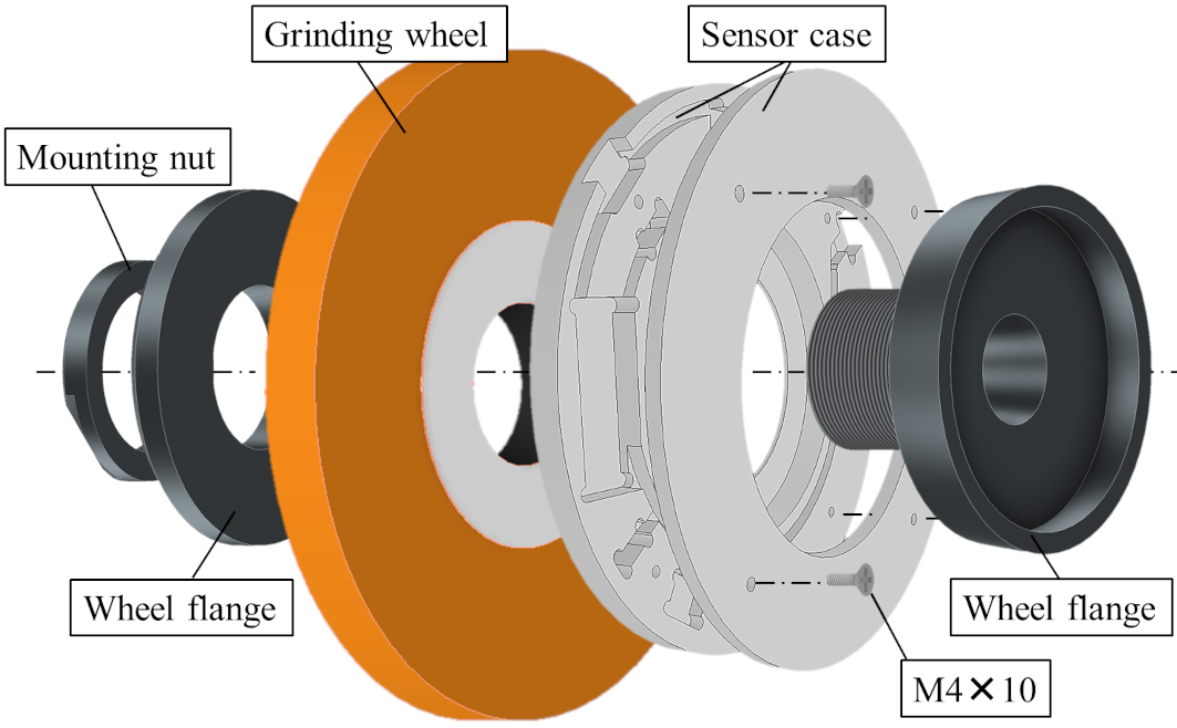
Wireless measuring device for grinding vibrations.
1. Introduction
In grinding, continuous operation changes the grinding wheel condition and may cause machining defects 1. If changes in the wheel condition can be measured in-process, such defects may be prevented. Extensive research has examined in-process tool monitoring in machining 2,3 and grinding 4. Typical monitoring parameters in grinding include the grinding force, temperature, acoustic emission (AE), and wheel spindle current 5,6,7,8. A dynamometer is commonly used to measure the grinding force. Although the grinding wheel condition can be assessed from variations in the grinding force using a dynamometer, its application in mass-production environments is limited by the high cost of the equipment.
In this study, a method for monitoring the condition of a grinding wheel by measuring grinding vibrations using an accelerometer was investigated. This approach is motivated by the frequent occurrence of vibrations during grinding, which often leads to machining defects 9,10,11. In conventional grinding processes, vibrations are typically measured either by attaching an accelerometer to the workpiece or mounting it on the bearing housing of the wheel spindle. Although attaching an accelerometer to a workpiece is straightforward during surface grinding, it is difficult during cylindrical grinding, in which the workpiece rotates. Mounting an accelerometer on the spindle-bearing housing also presents challenges, as vibration attenuation through the bearings and increased noise can reduce the measurement accuracy.
To address these issues, a wireless vibration measurement device was developed with a sensor mounted directly on the grinding wheel. In previous studies, wheel conditions were monitored by attaching AE sensors 12,13,14 or temperature and force sensors 15 to the grinding wheel, and the effectiveness of these methods was demonstrated. Furthermore, research is underway on a device for the in-process monitoring of vibrations in cutting processes, which mounts an accelerometer on a tool holder and transmits measured data wirelessly 16,17,18,19. In this study, this concept is extended to grinding by applying the same approach to the vibration measurement of a grinding wheel, thereby developing an in-process monitoring technique for grinding operations.
Two methods were investigated to process the measured data using the developed system. Grinding experiments were conducted under various conditions to verify the effectiveness of calculating the anomaly score using a neural network 20,21 within the microcontroller of the developed device, which is described as an edge-computing system.
2. Data Transmission and Processing Methods for Wireless Grinding Vibration Measurement System
In this study, two types of wireless measurement methods were developed that can be switched by reprogramming the microcontroller. The first is a raw data transmission method in which acceleration values obtained from two accelerometers are continuously transmitted to a personal computer (PC) via Wi-Fi. The second is an edge-computing method 22, in which a compact microcontroller within the measurement device computes an anomaly score and transmits only the score to a PC via Wi-Fi. The raw data transmission method ensures that the acceleration data received by the PC can be analyzed in various ways. However, its disadvantages include a large volume of data transmission, the resulting load on the PC and network, and the potential for data loss. In contrast, the edge-computing method calculates the anomaly score within the microcontroller that acquires the grinding vibration data, and only the computed result is transmitted to the PC. Although this method does not allow a detailed analysis of the raw acceleration data, it imposes a much smaller communication load and is, therefore, more suitable for mass-production environments. The anomaly score was computed using an autoencoder 23,24,25 based on neural network technology. An autoencoder compresses the characteristic features of the input data into a latent representation in the hidden layer through training and reconstructs the data to its original dimensionality at the output. As a result, when data representing a changed or abnormal state are input, the difference between the input and the reconstructed output increases. A notable feature of the autoencoder is that it performs unsupervised learning using only normal-state data for training. This makes it suitable for detecting changes in the grinding vibration.
3. Experimental Apparatus
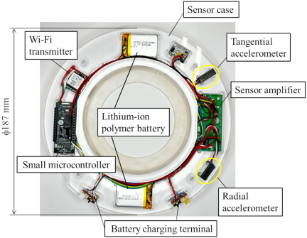
Fig. 1. Wireless measuring device for grinding vibrations.
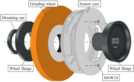
Fig. 2. Grinding wheel and wireless measuring device for grinding vibrations.
Figure 1 shows the wireless grinding vibration measurement device developed in this study. The grinding wheel measured \(\phi 205\times 19\) mm, whereas the acrylic housing of the developed device measured \(\phi 187\times 15\) mm. The device comprises two accelerometers (ACH-01, TE Connectivity Ltd.), an amplifier, a compact microcontroller (Spresense, Sony), a Wi-Fi module (iS110B, IDY), and two lithium-ion batteries (3.7 V, 400 mAh). All components were arranged within an acrylic housing to ensure rotational balance. Fig. 2 illustrates the method used to mount the device on a grinding wheel. The device was clamped between the grinding wheel flange and the wheel. The total mass of the developed device is 326 g, which is lightweight compared with the combined mass of the grinding wheel and flange (3 kg). The accelerometers were oriented to measure the vibrations of the wheel in both the radial and tangential directions. Accelerometers employ a piezoelectric sensing mechanism with a bandwidth of 2 Hz–20 kHz. The amplification circuit for the accelerometers used an operational amplifier (LF353) powered by positive and negative supplies from the lithium-ion batteries. The amplifier circuit was miniaturized to \(56\times 24\) mm using surface-mounted devices. Acceleration signals were fed from the amplifier circuit to the analog input of the microcontroller. Two measurement methods were implemented, which were selectable by reprogramming the microcontroller: a raw data transmission method and an edge computing method. The raw data transmission method uses open-source software 26 that utilizes the multitasking capability of the microcontroller to perform the analog-to-digital conversion of acceleration signals and Wi-Fi data transmission simultaneously. The sampling frequency was 48 kHz for the single-channel measurement (0.021 ms interval) and 24 kHz for the dual-channel measurement (0.042 ms interval). The sampling interval for the two channels was twice that of the single channel to ensure system stability during measurement. The battery life in the raw data transmission method was 4.1 h, primarily owing to the high power consumption of Wi-Fi transmission. In the edge computing method, the transmission interval of the anomaly score to the PC was set to 0.05 s (20 Hz) owing to the limited computational capabilities of the microcontroller. Consequently, the communication volume was reduced to \(1/\textrm{2,400th}\) of that in the raw data transmission method, extending the battery-powered operating time to 6.5 h. This represents a 1.6-fold increase compared to the raw data transmission method.
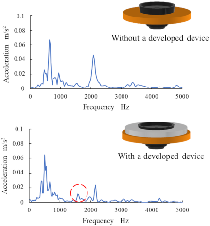
Fig. 3. Natural frequency of the wireless measuring device for grinding vibrations.
A preliminary experiment was conducted to measure the change in the natural frequency of the grinding wheel caused by the attachment of the developed device. Fig. 3 shows the measured natural frequencies of the grinding wheel with and without the installed device. It can be observed from the figure that a peak appears at approximately 1,610 Hz when the device is attached. This peak closely matched the natural frequency of the developed device, which was calculated to be 1,580 Hz using the finite element method.
A surface-grinding machine (PSG52DX, Okamoto Machine Tool Works, Ltd.) shown in Fig. 4 was used. The experimental conditions are listed in Table 1. The rotational speed of the grinding wheel was 3,000 min\(^{-1}\) (50 Hz). The workpiece material was S45C, with dimensions of 80 mm in the feed direction and 15 mm in the wheel width direction, with the latter being smaller than the wheel width. A solution-type grinding fluid (Noritake Cool NK-Z) diluted to 3% was used. During the experiments, the vibrations were measured using the developed device, and the grinding forces were simultaneously recorded using a three-component dynamometer (9254, Kistler) mounted beneath the workpiece.
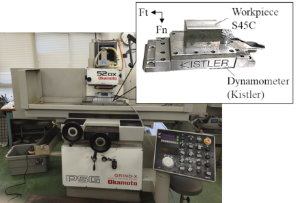
Fig. 4. Experimental equipment.
| Grinding wheel | WA80J8V36R, WA80N8V36R |
| Grinding wheel dimensions | \(\phi\)205 mm \(\times\) 19 mm |
| Workpiece | S45C |
| Workpiece dimensions | 80 mm \(\times\) 15 mm |
| Rotational speed of wheel | 3,000 min\(^{-1}\) |
| Grinding speed \(V_{g}\) | 32.2 m/s |
| Workpiece speed \(V_{w}\) | 0.05–0.22 m/s |
| Depth of cut \(d\) | 2, 4, 6 μm |
4. Experimental Results
4.1. Measurement Experiments Using a Raw Data Transmission Method
Machining experiments were conducted in which tangential and radial accelerations were measured at 24 kHz (0.042 ms interval) and transmitted to a PC in real time via Wi-Fi. A WA80J8V36R grinding wheel (Noritake Co., Ltd.) was used. The workpiece speed was set to 0.22 m/s, the depth of cut to 2 μm, and a single pass was performed under down-cut conditions. Prior to the experiments, the grinding wheel was carefully balanced, and sufficient zero-cut passes were performed. The received radial and tangential acceleration signals are presented in Figs. 5(a) and (b). After the experiments, frequency analyses of the radial and tangential acceleration data were performed on a PC, and the results are shown in Figs. 6(a) and (b). In the frequency analysis, data were acquired up to 12 kHz; however, Figs. 6(a) and (b) display only up to 6 kHz because of the low amplitudes in the higher-frequency range. From Figs. 5(a) and (b), a clear distinction can be observed between the acceleration signals during idle rotation and grinding. Peaks corresponding to the wheel rotation period of 0.02 s were evident in both the radial and tangential directions. In addition, the radial acceleration exhibited a larger amplitude. In the frequency-domain results shown in Figs. 6(a) and (b), no characteristic peaks other than those associated with the rotational frequency of the wheel were observed. To observe the variations in acceleration in real time, the accumulated absolute value of acceleration \(A\) was calculated using Eq. (1) and displayed on a PC monitor. Here, \(\Delta t\) denotes the sampling interval of the acceleration measurement (0.042 ms), \(a(n\Delta t)\) is the acceleration at time \(n\Delta t\), \(A\) is the accumulated absolute acceleration value, and \(N\) is the number of samples used for accumulation.
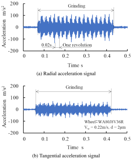
Fig. 5. Measurement results of acceleration.
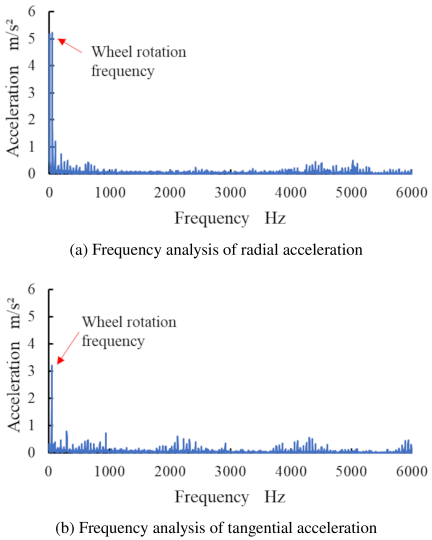
Fig. 6. Results of the frequency analysis.
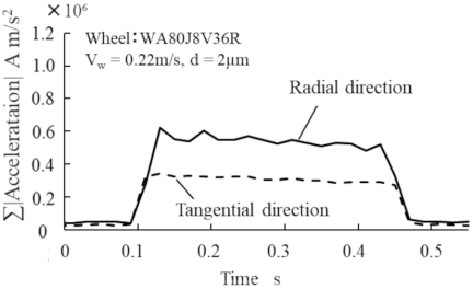
Fig. 7. Accumulated value of acceleration.
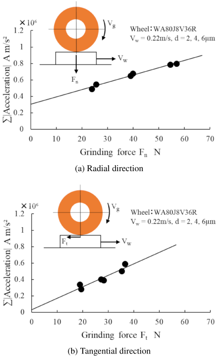
Fig. 8. Relationship between the grinding force and the integrated value of acceleration.
Figure 7 shows the temporal variation of the accumulated value obtained by setting the number of samples to \({N=480}\), corresponding to the grinding wheel rotational period \({T=0.02}\) s, so that the acceleration is accumulated once every period. In the raw data transmission method, in which all sampled acceleration data are stored directly on a PC, the computational load on the PC becomes substantial. Therefore, instantaneous acceleration values are not shown in real-time displays. Instead, the accumulated values that require far fewer display updates are presented to reduce the PC load. It is evident from the figure that the magnitude of the acceleration during grinding was successfully captured and that the radial acceleration was greater than the tangential acceleration. Using the same experimental setup (as in Fig. 6), the grinding depth was varied among 2, 4, and 6 μm.
Figure 8 illustrates the relationship between the accumulated absolute acceleration and the grinding force. Fig. 8(a) focuses on the radial acceleration versus the normal force \(F_{n}\), while Fig. 8(b) presents the tangential acceleration versus the tangential force \(F_{t}\). In both cases, the respective acceleration values exhibit a linear relationship with their corresponding grinding forces. Notably, the acceleration values obtained by extrapolating the regression lines to zero force in Fig. 8(a) exceeded the idling level (Fig. 7), confirming an increase in vibration upon contact.
The proposed system enables the estimation of both \(F_{n}\) and \(F_{t}\) through acceleration measurements provided that calibration is performed beforehand under specific grinding conditions.
4.2. Measurement Experiments Using an Edge-Computing Method
Measurement experiments were conducted using an edge-computing approach. In this method, all computations are performed within the developed device, and only the processed results are transmitted to a PC via Wi-Fi. An autoencoder was used to calculate the anomaly scores during the experiment. The architecture of the autoencoder is illustrated in Fig. 9. The input layer consisted of 128 data points, the hidden layer comprised three stages, and the output layer also contained 128 data points. A rectified linear unit (ReLU) function is used as the activation function. The input data for the autoencoder were obtained from the tangential acceleration measured at a sampling frequency (Fs) of 48 kHz with a fast Fourier transform (FFT) size (\(N\)) of 1,024. Frequency analysis was performed on the microcontroller within the developed device, and 128 data points up to 6,000 Hz were used, corresponding to a frequency resolution of \({\Delta f}\) (\(=\) Fs/N) of 46.9 Hz. A Hamming window with 50% overlap was applied during the FFT processing. A moving average process was applied to the FFT results to improve the signal-to-noise ratio and reduce random noise. The number of input data points was limited to 128 owing to memory constraints of the microcontroller. The frequency range used for the data analysis can be arbitrarily selected up to 24 kHz by modifying the program 27. Normal data for training the autoencoder were obtained from the acceleration signals measured while the grinding wheel rotated with the supplied coolant. Seventy datasets were used for training, and 30 were used for evaluation, with a total acquisition time of approximately two minutes. Anomaly scores were calculated using the root mean square error (RMSE), determined using Eq. (2), where \(n\) is the number of data points, \(x_{i}\) is the FFT-processed acceleration data, and \(x_{o}\) is the output generated by the autoencoder. Fig. 10 shows ten examples of frequency-domain data used for training. A distinct peak is observed near 50 Hz, corresponding to the rotational speed of the grinding wheel.
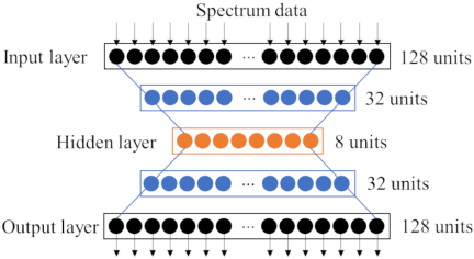
Fig. 9. Structure of the autoencoder.
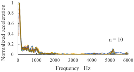
Fig. 10. Spectrum data used for training.
First, the variation in the RMSE caused by the rotation of the grinding wheel during idling was measured. The experimental results are shown in Figs. 11(a)–(c). Fig. 11(a) shows the temporal change in the rotational speed of the grinding wheel, whereas Fig. 11(b) shows the corresponding change in the RMSE. In this experiment, a stop command was issued, causing the rotational speed to gradually decrease from 3,000 min\(^{-1}\) until the wheel came to a complete halt. After remaining stationary for 20 s, a start command was applied to initiate rotation. The results indicated that the anomaly scores increased as the rotational speed approached zero. Fig. 11(c) presents the RMSE measurement results within a spindle speed range of 1,000 to 3,000 min\(^{-1}\). The figure shows that the variation in the RMSE was minimal within this range. These results indicate that while the developed device is capable of detecting a complete spindle stop, it is not sensitive enough to detect changes in the rotational speed within the range of 1,000 to 3,000 min\(^{-1}\).
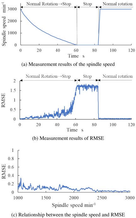
Fig. 11. RMSE measurement of grinding wheel rotational speed.
Next, the progression of the RMSE during grinding was measured. The experiment was conducted under the same conditions as those shown in Fig. 5 using a single-pass grinding operation. Fig. 12(a) presents the RMSE transmitted to a PC via Wi-Fi for depths of cut 2 μm and 6 μm. The normal grinding force \(F_{n}\) measured using a dynamometer is shown in Fig. 12(b), whereas the tangential grinding force \(F_{t}\) is shown in Fig. 12(c). As shown in Fig. 12(a), the RMSE remained low in the non-contact state but increased during grinding. Furthermore, increasing the depth of cut from 2 μm to 6 μm causes the RMSE to increase accordingly. It took 0.2 s for the RMSE to reach its peak value, owing to the application of the moving average. Notably, the RMSE value may not reach its peak if the grinding time is shorter than this duration.
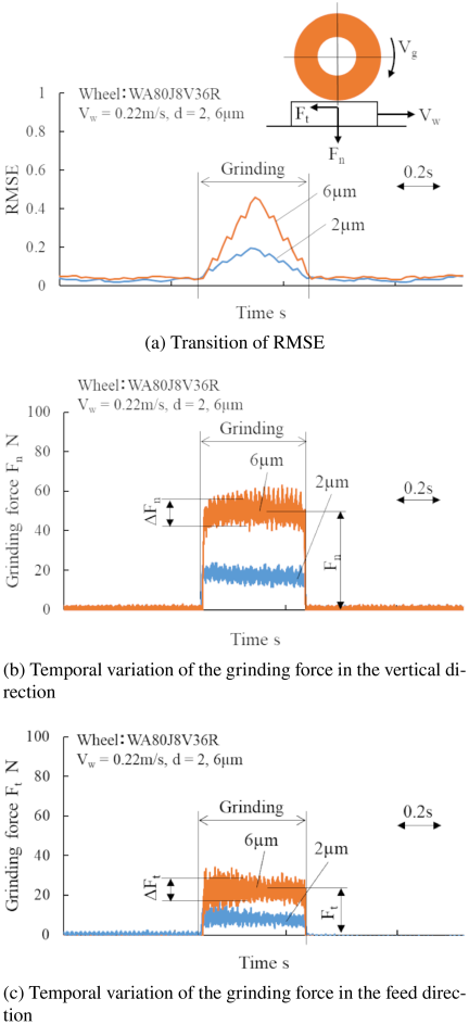
Fig. 12. Temporal variation of the RMSE and grinding force.
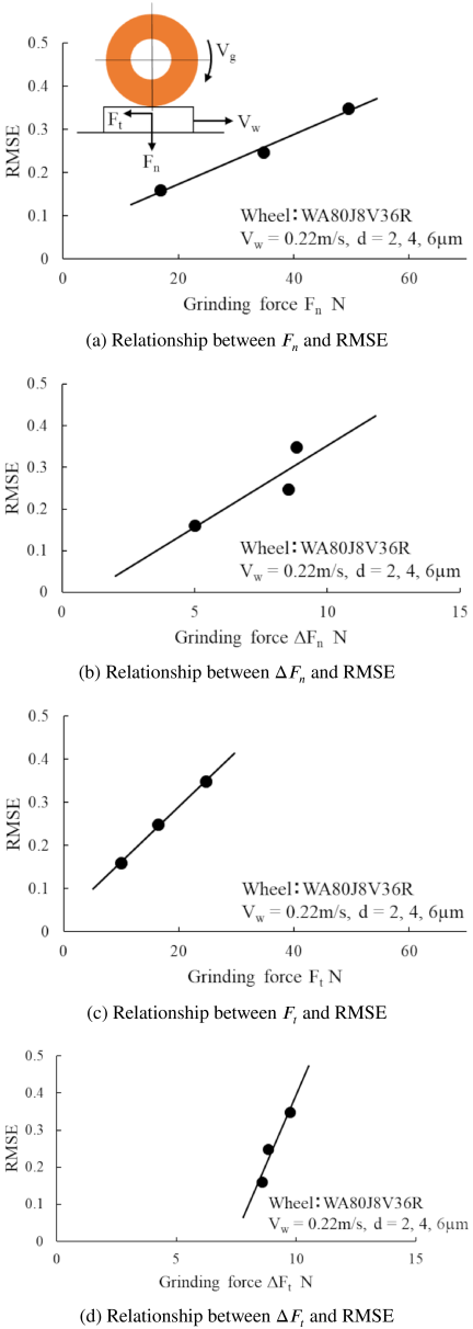
Fig. 13. Relationship between the grinding force and RMSE.
The relationship between the grinding forces and the peak RMSE resulting from larger infeed depths was investigated. Experiments were conducted at infeed depths of 2, 4, and 6 μm. Figs. 13(a) and (b) show the relationship between the normal grinding force \(F_{n}\) and the peak RMSE and between its amplitude \(\Delta F_{n}\) and this value, respectively. Similarly, Figs. 13(c) and (d) present the relationship between tangential grinding force \(F_{t}\) and its amplitude \(\Delta F_{t}\). From Fig. 13, it is evident that both the grinding forces and their amplitudes increase with increasing infeed depth. A linear relationship is observed between the peak RMSE and these forces. These findings suggest that the magnitude of the grinding forces can be estimated using the peak RMSE measured using the developed system under the same grinding conditions.
Next, the changes in the RMSE owing to the grinding-wheel condition were measured. After dressing the wheel, a grinding experiment was performed with an infeed depth of 2 μm until a total infeed of 2 mm was reached. The workpiece was moved only in the left-right direction at a speed of 0.05 m/s. Fig. 14(a) shows the relationship between the total infeed and RMSE, whereas Fig. 14(b) presents the RMSE variation at the beginning of grinding and immediately before reaching a total infeed of 2 mm. Fig. 14(c) illustrates the relationship between the total infeed and normal grinding force \(F_{n}\). Both Figs. 14(a) and (c) indicate that the RMSE and normal grinding force increase as the total infeed increases. In addition, Fig. 14(b) clearly distinguishes the RMSE waveform during the contact and non-contact conditions. An RMSE value of approximately 0.1 corresponds to the non-contact state in which the wheel is not engaged with the workpiece. From Fig. 14(b), it is evident that the RMSE during grinding differs significantly between the initial stage and immediately before reaching a total infeed of 2 mm. These results demonstrate that the developed system can detect changes in grinding-wheel conditions.
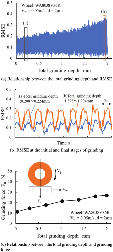
Fig. 14. Experimental results of grinding under reference condition (\(V_{w}=0.05\) m/s, \(d =2\) μm).
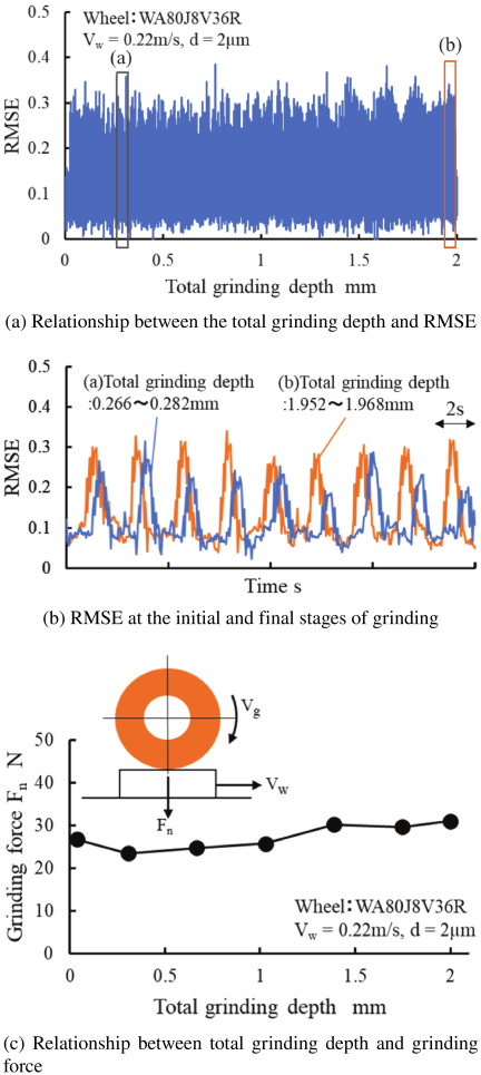
Fig. 15. Experimental results of grinding with varying workpiece speeds (\(V_{w}=0.22\) m/s, \(d=2\) μm).
Figure 15 shows the experimental results obtained when the workpiece speed in the experiment of Fig. 14 was increased from 0.05 m/s to 0.22 m/s. As the workpiece speed increased, the maximum grain depth of the cut increased by 4.4 times. Fig. 15(a) shows the relationship between the total depth of cut and RMSE, whereas Fig. 15(b) illustrates the evolution of the RMSE at the beginning of grinding and immediately before the total depth of the cut reached 2 mm. Fig. 15(c) shows the relationship between the total depth of cut and the normal grinding force \(F_{n}\). A comparison of Figs. 15(a) and (c) with Figs. 14(a) and (c) shows that the RMSE was high in the early stages of grinding, although it may not have reached its peak because of the moving average processing. Similarly, the normal grinding force exhibited high values during the initial stage. Furthermore, even as the total depth of cut increased, both the RMSE and normal grinding force exhibited only minor variations.
Figure 16 shows the experimental results obtained when the depth of cut per pass in the experiment shown in Fig. 14 increased from 2 μm to 6 μm. As the depth of cut per pass increases, the maximum grain depth of the cut increases by 1.7 times. Fig. 16(a) shows the relationship between the total depth of cut and RMSE, whereas Fig. 16(b) illustrates the evolution of the RMSE at the beginning of grinding and immediately before the total depth of cut reached 2 mm. Fig. 16(c) shows the relationship between the total depth of cut and the normal grinding force \(F_{n}\). From Figs. 16(a) and (c), it can be observed that both the RMSE and normal grinding force exhibit larger values in the early stage of grinding compared to Fig. 14. Immediately before the total depth of cut reached 2 mm, both the RMSE and the normal grinding force exhibited almost the same values, as shown in Figs. 14 and 16. Furthermore, as shown in Figs. 16(b) and (c), no significant changes in the RMSE or grinding force were observed between the initial and final stages of grinding.
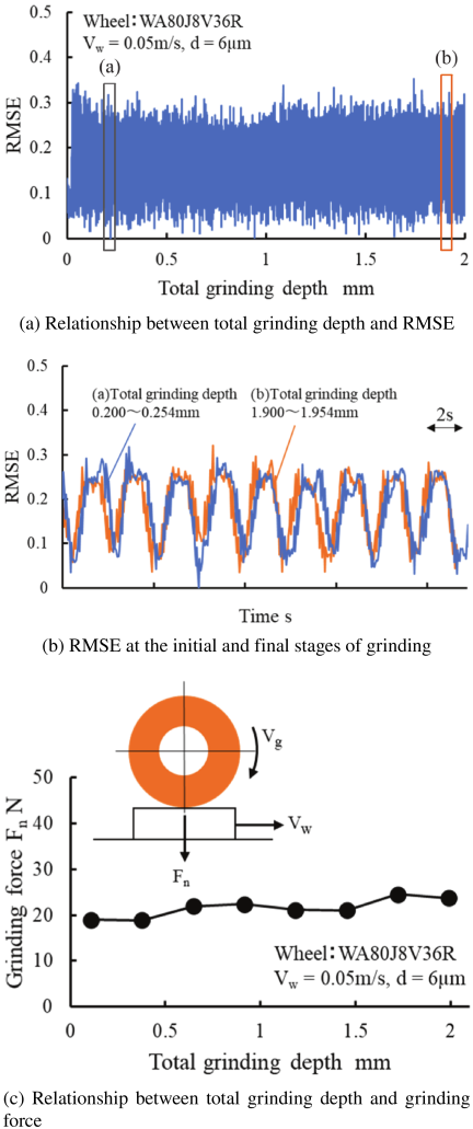
Fig. 16. Experimental results of grinding with varying depth of cut (\(V_{w}=0.05\) m/s, \(d=6\) μm).
Based on the experimental results shown in Figs. 14–16, it is suggested that by observing the RMSE obtained from the developed system, changes in the grinding-wheel condition can be estimated at a level comparable to that achieved by measuring the grinding force.
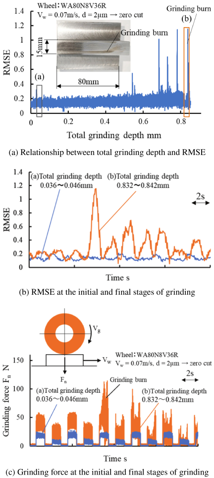
Fig. 17. Experimental results of grinding under condition conducive to grinding burn.
To investigate the detection of grinding burns, grinding experiments were conducted under the conditions described in our previous studies to induce this phenomenon. A different grinding wheel, WA80N8V36R (Noritake Co., Ltd.), was used. The workpiece speed was set to 0.07 m/s, and the depth of cut was repeatedly varied in a sequence of 2 μm followed by a zero-cut. In this experiment, grinding burns occurred on the machined surface at a total cut of 0.85 mm, as shown in the photograph of the workpiece in Fig. 17(a), after which the experiment was terminated. Fig. 17(a) shows the relationship between the total depth of cut and the RMSE. Fig. 17(b) illustrates the evolution of the RMSE at the beginning and immediately before the end of machining. Fig. 17(c) shows the corresponding evolution of the normal grinding force \(F_{n}\). In Fig. 17(a), an abnormal RMSE waveform is observed when a grinding burn occurs at a total grinding depth of 0.85 mm. Additionally, abnormal values were observed in the RMSE waveform at the total grinding depths of 0.69 mm, 0.74 mm, and 0.79 mm. As the identification of grinding burns relies on the operator’s subjective evaluation, it remains uncertain whether the observed RMSE anomalies correspond precisely to the occurrence of burns in this experiment. In the waveform obtained immediately before the end of the grinding, as shown in Fig. 17(b), an abnormal RMSE pattern presumably associated with grinding burns was observed, indicating that a machining anomaly had already occurred at this stage. Based on the normal grinding forces shown in Fig. 17(c), the difference between the 2 μm depth of cut and the zero-cut is clearly visible at the beginning of machining. The abnormal grinding force was recorded immediately before the machining ended. The RMSE waveform exhibits the same trend as the grinding force waveform. It is expected that, as the amplitude of the grinding force increases, the vibration of the grinding wheel also increases. Although the specific reason for the increased force amplitude during grinding burn remains unidentified in this experiment, the increase in force amplitude appears to coincide with the increase in RMSE. In this experiment, the vibration increased with the occurrence of grinding burns. Therefore, grinding burns can also be detected by measuring the accumulated absolute acceleration, which is an indicator given by Eq. (1).
5. Conclusion
In this study, a wireless grinding vibration measurement system was developed. The conclusions of this study are as follows.
-
1.
The system consisted of two accelerometers, an amplifier, a compact microcontroller, a Wi-Fi transmitter, and two batteries, all housed in an acrylic case. It was mounted on the grinding wheel of a surface-grinding machine to measure the grinding vibrations.
-
2.
Using the developed system, the acceleration in two directions was measured at a sampling frequency of 24 kHz and transmitted to a PC in real time. A program was developed to accumulate the absolute value of the received acceleration for each wheel revolution and to display the results on a PC in real time. The accumulated values exhibited a linear relationship with the magnitude of the grinding force.
-
3.
The acceleration measured by the developed system was processed using an autoencoder implemented on a microcontroller to compute the anomaly scores transmitted to a PC at intervals of 0.05 s. When the rotational speed of the grinding wheel during the idle operation was varied, the anomaly scores increased as the rotational speed approached zero.
-
4.
Anomaly scores were measured while varying the depth of cut of the grinding wheel into the workpiece. The experimental results showed a correlation between the anomaly scores and the grinding force. Furthermore, in experiments in which grinding was continued under identical machining conditions, cases in which the anomaly scores increased as the grinding wheel condition changed were observed. An increase in anomaly scores was also observed when grinding burns occurred.
Acknowledgments
The authors thank Tomonobu Hayakawa of Sony Semiconductor Solutions Corporation for his support of this research.
- [1] M. Fujimoto, T. Ninomiya, and H. Mieno, “Effect of wear behavior of grain cutting edges on chatter vibration in creep feed grinding,” J. Jpn. Soc. Abras. Technol., Vol.68, No.1, pp. 33-38, 2024 (in Japanese). https://doi.org/10.11420/jsat.68.33
- [2] F. Bleicher, D. Biermann, W.-G. Drossel, H.-C. Moehring, and Y. Altintas, “Sensor and actuator integrated tooling systems,” CIRP Ann., Vol.72, No.2, pp. 673-696, 2023. https://doi.org/10.1016/j.cirp.2023.05.009
- [3] K. Ohashi, “Measuring techniques and their applications in grinding process,” J. Jpn. Soc. Precis. Eng., Vol.84, No.2, pp. 138-141, 2018 (in Japanese). https://doi.org/10.2493/jjspe.84.138
- [4] Y. Kurahashi, “The latest machining process monitoring technology,” J. Jpn. Soc. Abras. Technol., Vol.62, No.5, pp. 250-253, 2018.
- [5] J. Hsieh and I. Inasaki, “Monitoring of dressing and grinding process with acoustic emission signals,” Trans. Jpn. Soc. Mech. Eng. Ser. C, Vol.51, No.468, pp. 2174-2179, 1985 (in Japanese). https://doi.org/10.1299/kikaic.51.2174
- [6] Y. Nagasu, K. Yamada, K. Maruyama, H. Tsuboi, and M. Kitahara, “Development of determination system for grinding process status by acoustic emission sensor,” Res. Rep. Nagano Prefect. Gen. Ind. Technol. Cent., No.16, pp. 1-5, 2021 (in Japanese).
- [7] K. Yamashita, H. Kondo, and H. Koike, “Estimation of stability of grinding process by acoustic emission sensor,” Rep. Ind. Technol. Cent. Tochigi Prefect., No.21, pp. 66-70, 2024 (in Japanese).
- [8] T. Kasuga et al., “Studies on workpiece surface roughness estimation technology using AE signals during grinding,” Proc. JSPE Semestrial Meet., pp. 567-568, 2024 (in Japanese). https://doi.org/10.11522/pscjspe.2024S.0_567
- [9] Y. Tani, “Vibration in grinding,” Seisan Kenkyu, Vol.34, No.3, pp. 77-82, 1982.
- [10] I. Inasaki and S. Yonezu, “Chatter vibration in flat and cylindrical grinding,” J. Jpn. Soc. Precis. Eng., Vol.35, No.408, pp. 47-53, 1969 (in Japanese). https://doi.org/10.2493/jjspe1933.35.47
- [11] S. Okuyama, “Grinding engineering for young engineers: Part 10 causes of chatter vibration and its suppression,” J. Jpn. Soc. Abras. Technol., Vol.59, No.11, pp. 651-654, 2015.
- [12] M. Wakuda, I. Inasaki, K. Ogawa, and M. Takahara, “Monitoring of the grinding process with an AE sensor integrated CBN wheel,” J. Jpn. Soc. Precis. Eng., Vol.59, No.2, pp. 275-280, 1993 (in Japanese). https://doi.org/10.2493/jjspe.59.275
- [13] B. Karpuschewski, M. Wehmeier, and I. Inasaki, “Grinding monitoring system based on power and acoustic emission sensors,” CIRP Ann., Vol.49, No.1, pp. 235-240, 2000. https://doi.org/10.1016/S0007-8506(07)62936-9
- [14] B. Varghese, S. Pathare, R. Gao, C. Guo, and S. Malkin, “Development of a sensor-integrated ‘intelligent’ grinding wheel for in-process monitoring,” CIRP Ann., Vol.49, No.1, pp. 231-234, 2000. https://doi.org/10.1016/S0007-8506(07)62935-7
- [15] E. Brinksmeier, C. Heinzel, and L. Meyer, “Development and application of a wheel based process monitoring system in grinding,” CIRP Ann., Vol.54, No.1, pp. 301-304, 2005. https://doi.org/10.1016/S0007-8506(07)60108-5
- [16] R. Matsuda, M. Shindou, T. Hirogaki, and E. Aoyama, “Monitoring of rotational vibration in tap and endmill processes with a wireless multifunctional tool holder system,” Int. J. Automation Technol., Vol.12, No.6, pp. 876-882, 2018. https://doi.org/10.20965/ijat.2018.p0876
- [17] R. Matsuda, M. Shindou, T. Hirogaki, and E. Aoyama, “Study on monitoring tool temperature and vibration in drilling and countersinking processes with a multi-functional wireless communication tool holder system,” Trans. JSME, Vol.85, No.872, Article No.18-00176, 2019 (in Japanese). https://doi.org/10.1299/transjsme.18-00176
- [18] T. Yamamoto, R. Matsuda, M. Shindou, T. Hirogaki, and E. Aoyama, “Monitoring of vibrations in free-form surface processing using ball nose end mill tools with wireless tool holder systems,” Int. J. Automation Technol., Vol.15, No.3, pp. 335-342, 2021. https://doi.org/10.20965/ijat.2021.p0335
- [19] J. V. Abellan-Nebot and F. Romero Subirón, “A review of machining monitoring systems based on artificial intelligence process models,” Int. J. Adv. Manuf. Technol., Vol.47, No.1, pp. 237-257, 2010. https://doi.org/10.1007/s00170-009-2191-8
- [20] L. Hou and N. W. Bergmann, “Novel industrial wireless sensor networks for machine condition monitoring and fault diagnosis,” IEEE Trans. Instrum. Meas., Vol.61, No.10, pp. 2787-2798, 2012. https://doi.org/10.1109/TIM.2012.2200817
- [21] K. Kato, K. Utsumi, K. Nishikawa, and A. Nomura, “Development of wireless cutting vibration monitoring device fixed to tool holder,” Int. J. Abras. Technol., Vol.11, No.1, pp. 1-16, 2022. https://doi.org/10.1504/IJAT.2022.125266
- [22] Y. Okayama, “Outline of edge computing that supports cyber physical system,” Oyo Buturi, Vol.89, No.9, pp. 535-538, 2020 (in Japanese). https://doi.org/10.11470/oubutsu.89.9_535
- [23] M. Uchida, S. Ishida, T. Tabaru, and H. Miyamoto, “Anomaly detection of rotary vacuum pump using thin AE sensor and reconstruction error of autoencoder,” Trans. Soc. Instrum. Control Eng., Vol.54, No.7, pp. 599-605, 2018 (in Japanese). https://doi.org/10.9746/sicetr.54.599
- [24] K. Oda, H. Suwa, and K. Murakami, “Cutting anomaly detection in end-milling by multimodal variational autoencoder,” Trans. JSME, Vol.89, No.918, Article No.22-00290, 2023 (in Japanese). https://doi.org/10.1299/transjsme.22-00290
- [25] S. Asahi et al., “Proposal of failure prediction method of factory equipment by vibration data with recurrent autoencoder,” Trans. JSME, Vol.86, No.891, Article No.20-00020, 2020 (in Japanese). https://doi.org/10.1299/transjsme.20-00020
- [26] T. Hayakawa, “Spresense-Playground.” https://github.com/TomonobuHayakawa/Spresense-Playground/tree/master/IntegrationWithProcessing/FrequencyCharacteristi [Accessed August 17, 2026]
- [27] Sony Semiconductor Solutions Corporation and Y. Ota, “Low-Power Edge AI with SPRESENSE,” O’Reilly Japan, 2022.
This article is published under a Creative Commons Attribution-NoDerivatives 4.0 Internationa License.