Research Paper:
Tree Stem Perimeter Estimation for Forestry Robots via Residual Learning and LiDAR–RGB Fusion
Md Abul Munjer*,†
 , Chi Jie Tan*
, Vincent Boufaroua*
, Abbe Mowshowitz**
, and Eiji Hayashi*
, Chi Jie Tan*
, Vincent Boufaroua*
, Abbe Mowshowitz**
, and Eiji Hayashi*
*Faculty of Computer Science and System Engineering, Kyushu Institute of Technology
680-4 Kawazu, Iizuka, Fukuoka 820-0067, Japan
†Corresponding author
**Department of Computer Science, The City College of New York
New York, USA

Accurate estimation of tree stem perimeter is essential for robotic forest mapping and inventory applications. While light detection and ranging (LiDAR)–camera fusion enables automated stem detection and geometric reconstruction, perimeter estimates derived from partial LiDAR observations exhibit systematic bias due to occlusions, limited angular coverage, and violations of ideal cylindrical assumptions. These effects introduce systematic errors that cannot be fully resolved by geometric reconstruction or temporal smoothing alone. This paper proposes a residual learning framework that enhances geometric perimeter estimation by learning a data-driven correction term while preserving the interpretability of the underlying model. A mobile robot equipped with a three-dimensional LiDAR and an RGB camera collects synchronized data in forest environments. Tree stems are detected in RGB images and associated with LiDAR points through calibrated projection. A geometric baseline perimeter is computed by fitting a circular model to a diameter-at-breast-height cross-section extracted from incomplete LiDAR observations. A shallow multilayer perceptron then predicts the residual between the geometric estimate and manually measured ground-truth perimeter using observation-derived features. Filtering improves stability but does not remove systematic bias, whereas residual learning achieves consistent bias correction. Experimental results demonstrate reductions exceeding 40% in both mean absolute and root mean squared errors, together with a substantial improvement in the coefficient of determination from 0.48 to 0.86. Error distributions become more centered and consistent across varying sensing distances and stem sizes, confirming robust generalization to unseen trees. The proposed method operates as a lightweight post-processing module, making it suitable for real-time deployment on mobile forestry robots.
1. Introduction
Forestry sectors worldwide are increasingly affected by labor shortages, driven by aging workforces, rising operational costs, and declining availability of skilled field surveyors 1,2. At the same time, sustainable forest management remains essential for long-term ecosystem health, carbon regulation, and efficient use of natural resources. Improving the efficiency, consistency, and energy utilization of forest monitoring operations has therefore become an urgent priority, particularly as forestry operations expand in scale and complexity.
Conventional forest inventory tasks—such as manual measurement of tree diameter or perimeter—are labor-intensive, time-consuming, and difficult to scale across large or dense forest areas 3. These challenges have accelerated interest in autonomous mobile robots capable of performing forest mapping and measurement tasks with minimal human intervention 4. Accurate tree mapping and stem perimeter (or radius) estimation are fundamental to forest inventory, biomass estimation, growth analysis, and autonomous navigation in cluttered environments 5,6,7,8,9,10. For mobile robots operating in forests, stem geometry provides not only ecological metrics but also critical structural cues for localization, obstacle avoidance, and path planning 11.
Reliable perimeter or radius estimation from onboard sensors remains a central requirement for robotic forestry applications. Since accurate perimeter estimation in forests requires robot motion to capture multiple viewpoints, robots must estimate stem size in real time from onboard sensors during navigation.
Most existing approaches rely on geometric stem estimation, typically fitting circles or cylinders to light detection and ranging (LiDAR) point clouds acquired at breast height or other fixed elevations. These methods have demonstrated high accuracy under controlled conditions and dense, uniform angular coverage around the stem, such as in terrestrial laser scanning (TLS) setups 12,13,14.
While high-precision tree stem measurements have been achieved using TLS and photogrammetry-based approaches, these methods typically operate under controlled acquisition conditions with dense and near-complete geometric coverage. For example, centimeter-level accuracy can be achieved when dense point clouds are available 15. Similarly, both laser scanning and image-based reconstruction methods can accurately estimate tree diameters under static and nearly complete angular coverage of the stem 16.
However, these approaches rely on assumptions that do not hold in mobile robotic scenarios. In contrast to static sensing setups, mobile platforms operating in forest environments encounter sparse, viewpoint-dependent, and partially occluded observations. As a result, only a limited portion of the stem surface is observed at any given time, leading to incomplete angular coverage and insufficient geometric constraints for reliable estimation. Unlike taking measurements in static environments, performance degrades substantially in mobile robotic scenarios, where measurements are sparse, viewpoint-dependent, and frequently occluded by vegetation or neighboring trees 17,18. Consequently, geometric estimators often exhibit systematic error, meaning that the estimated values are consistently higher or lower than the true values rather than randomly distributed.
Another key limitation of conventional approaches is the assumption that tree stems can be adequately modeled as ideal circular or cylindrical shapes. In real forests, stems deviate from these idealized forms due to natural asymmetry, buttress swell, bark irregularities, and growth variability. More importantly, mobile platforms rarely observe a full 360° cross-section of a stem 18. Instead, they capture LiDAR observations that cover only a portion of the stem circumference. In such cases, circle fitting methods attempt to infer the full shape from incomplete data, often relying on assumptions that do not hold in practice. This leads to systematic deviations in the estimated radius or perimeter.
The problem of incomplete angular coverage of the stem cross-section is therefore a dominant source of error in mobile LiDAR-based stem measurement. For example, when a robot observes a tree from one side, LiDAR points are collected only from the visible portion of the stem surface, while the opposite side remains unobserved due to occlusion or limited viewpoint limitation. As a result, the observed points represent only a partial section of the circular boundary rather than a full circle. When only a limited angular sector of a stem is observed, geometric fitting methods extrapolate missing regions using symmetry assumptions that do not hold in practice. Although several studies have proposed improved geometric heuristics to mitigate this issue, such methods remain fundamentally constrained by incomplete information and cannot fully eliminate systematic bias 19. Learning-based approaches provide a promising alternative for addressing this limitation. Instead of replacing geometric estimation, a residual learning approach can be used to model the consistent error between the estimated and true values. Since this error arises from structured geometric limitations rather than random noise, it can be learned from observation-derived features. Rather than replacing geometry entirely, residual neural networks can be used to model and correct the systematic errors produced by analytic estimators. This is particularly appropriate for stem perimeter estimation, where the dominant error arises from consistent geometric bias associated with partial observations, making the residual predictable from observed features.
In this work, a bias-aware perimeter estimation framework has been proposed for mobile robotic forest sensing. A shallow residual learning model is used to correct geometric perimeter estimates obtained from LiDAR–camera fusion. The method preserves the interpretability and computational efficiency of geometric fitting while improving accuracy by compensating for systematic errors caused by incomplete observations. The model operates as a lightweight post-processing module, learning to correct this bias without changing the geometric model. This hybrid formulation is well suited for real-time deployment on mobile robots and provides a practical solution for perimeter or radius estimation under partial arc observations.
The proposed framework is based on a LiDAR–RGB fusion pipeline, where tree stems are detected in RGB images using a deep learning-based object detector, and corresponding LiDAR points are associated through geometric projection. This enables the extraction of stem-specific point clouds for geometric analysis. Unlike system-level approaches that focus on mapping and localization, this work addresses a complementary limitation at the measurement level, namely the systematic bias introduced by incomplete observations. By introducing a residual learning formulation that corrects geometric estimates rather than replacing them, this work focuses on enabling reliable and bias-aware perimeter estimation for mobile robotic platforms operating under realistic sensing conditions, where incomplete observations are unavoidable.
2. Methodology
2.1. Robotic Platform and Sensor Configuration
The experimental platform used in this study is a mobile ground robot equipped with synchronized LiDAR, RGB, inertial, and positioning sensors for autonomous forest data acquisition. The complete robotic system and the geometric relationships between sensor frames are illustrated in Fig. 1. The robot is equipped with a Velodyne VLP-16 LiDAR mounted on a rigid vertical mast to provide full 360° three-dimensional range measurements of the surrounding environment. An Intel RealSense RGB camera is mounted below the LiDAR and oriented forward to capture visual observations of tree stems. Additional onboard sensors include an Xsens MTi-680G inertial measurement unit (IMU), an Emlid RTK-GPS module for global positioning, a wireless router for communication, and an Intel NUC computer that performs all onboard processing.
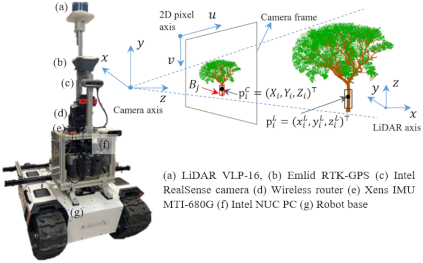
Fig. 1. Robotic platform and sensor coordinate frames for LiDAR–camera fusion.
All sensors are rigidly mounted and spatially calibrated with respect to a common robot base frame. Known extrinsic calibration parameters allow LiDAR points to be transformed into the camera coordinate system and projected onto the image plane. As illustrated in Fig. 1, each three-dimensional (3D) LiDAR point \(\boldsymbol{p}_{i}^{L} = (x_{i}^{L}, y_{i}^{L}, z_{i}^{L})^{\mathsf{T}}\) can be mapped into the camera frame and subsequently onto the two-dimensional (2D) image plane. The projected point is represented as \(p_{i}^{c} = (X_{i}, Y_{i}, Z_{i})^{\mathsf{T}}\), which corresponds to a pixel location \((u,v)\) in the image. Tree stems are detected in the RGB image as bounding boxes \(B_{j}\). A LiDAR point is associated with a detected stem if its projected pixel location falls within the corresponding bounding box \(B_{j}\). This establishes a correspondence between 3D LiDAR points and 2D image detections, effectively linking geometric measurements with semantic information. Through this LiDAR–RGB fusion process, the original point cloud is partitioned into stem-specific subsets, enabling robust extraction of tree stem points from the surrounding environment despite the presence of clutter and occlusions.
The robot operates under the Robot Operating System (ROS) 2 20 and supports autonomous navigation using a standard ROS 2 navigation stack. Wheel encoder data are fused with IMU measurements to provide continuous odometry estimation, which is used for motion control, trajectory execution, and temporal alignment of sensor data. Autonomous behaviors such as waypoint following, obstacle avoidance, and controlled scanning motions are executed through ROS 2 action interfaces. Odometry information is used exclusively to support autonomous operation and data collection consistency; it is not directly involved in the geometric perimeter estimation or learning-based correction stages described later.
During operation, the robot traverses forest environments while continuously collecting synchronized LiDAR point clouds and RGB images. Tree stems are detected in the RGB images using an onboard object detector, while the LiDAR sensor simultaneously captures the 3D structure of the scene. The calibrated sensor configuration enables direct association between visual detections and LiDAR points, forming the basis for tree-specific point cloud extraction and subsequent geometric processing.
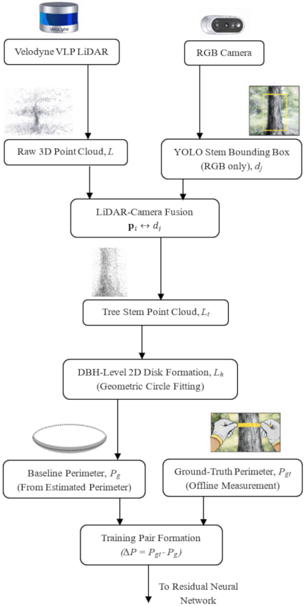
Fig. 2. Perimeter estimation and residual training target generation pipeline.
2.2. Geometric Perimeter Estimation for Data Collection
The proposed framework employs a geometric perimeter estimation pipeline to stem-specific LiDAR point clouds obtained through the LiDAR–camera fusion process. This stage generates baseline geometric estimates and corresponding ground-truth training pairs for subsequent residual learning. The complete processing flow for data generation and geometric baseline estimation is illustrated in Fig. 2. Raw 3D point clouds are acquired by the onboard LiDAR sensor, while tree stems are independently detected in RGB images using a You Only Look Once (YOLO)-based object detector 21,22,23.
The LiDAR–camera fusion process described in Section 2.1 is used to associate LiDAR points with detected stems, resulting in stem-specific point cloud subsets. These associated point sets serve as the input for geometric processing. By restricting the analysis to stem-specific LiDAR points, the effects of background clutter and non-stem structures are significantly reduced, enabling more reliable estimation of tree stem geometry. For each detected tree stem, a corresponding subset of LiDAR points is extracted. The resulting set of tree-associated LiDAR points is defined as in Eq. \(\eqref{eq:1}\).
A vertical filtering operation is applied to \(L_t\) to extract points within a narrow height band around breast height. The resulting subset \(L_h\) defined in Eq. \(\eqref{eq:2}\) represents a localized cross-section of the tree stem. The points in \(L_h\) are then projected onto the horizontal plane to form a 2D cross-section, which can be denoted as in Eq. \(\eqref{eq:3}\).
Due to occlusions, limited viewpoints, and forest clutter, the resulting cross-section typically forms a partial arc rather than a complete circular boundary. Nevertheless, a circular model is fitted to these points to obtain a geometric approximation of the stem cross-section. The circle parameters \((c_{x}, c_{y}, r_{g})\) are estimated by minimizing the least-squares objective as defined by Eq. \(\eqref{eq:4}\), where \((x_{i}, y_{i})\) represents the 2D cross-sectional points used for geometric fitting.
Expanding and introducing parameters \(\theta_{1} = 2x_{c}\), \(\theta_{2} = 2y_{c}\), and \(\theta_{3} = r^{2} - x_{c}^{2} - y_{c}^{2}\) in Eq. \(\eqref{eq:6}\) yields a linear form as shown in Eq. \(\eqref{eq:7}\), where \((x_{i}, y_{i})\) denotes the \(i\)-th observed LiDAR point in \(L_h\) onto the cross-sectional plane, and the parameters are defined as
For a set of \(N\) points, having the definitions \(A = [\begin{matrix}x_{i}& y_{i}& 1\end{matrix}]\), \(b = [x_{i}^{2} + y_{i}^{2}]\), and \(\theta = [\begin{matrix}\theta _{1}& \theta_{2}& \theta_{3}\end{matrix}]^{\mathsf{T}}\), the system can be expressed in matrix form as \(A\theta \approx b\) whose solution is given by \(\theta = (A^{\mathsf{T}}A)^{-1}A^{\mathsf{T}}b\). From the estimated parameters, the geometric quantities are recovered as \(x_{c} = \theta_{1}/2\), \(y_{c} = \theta_{2}/2\), and \(r = \sqrt{(x_{c}^{2} + y_{c}^{2} + \theta_{3})}\).
Although this algebraic least-squares formulation provides a closed-form solution, it is sensitive to incomplete and non-uniform point distributions Therefore, the nonlinear geometric formulation in Eq. \(\eqref{eq:4}\) is adopted for final estimation. The optimization is solved using a Levenberg–Marquardt algorithm, where the initial values of the circle parameters \((x_{c}, y_{c}, r)\) are obtained from the algebraic least-squares solution. The estimated radius \(r_g\) for a stem is then used to compute the geometric baseline perimeter \(P_{g} = 2\pi r_{g}\). This perimeter represents the baseline measurement obtained from partial LiDAR observations under idealized circular assumptions. For each tree, a corresponding ground-truth perimeter \(P_{gt}\) is measured offline using a diameter tape at the same reference height. The discrepancy between the geometric estimate and the manual measurement is expressed as a residual term as in Eq. \(\eqref{eq:8}\) which captures the systematic bias introduced by partial arc coverage and geometric assumptions.
The paired values (\(\boldsymbol{x}\), \(\Delta P\)), where \(\boldsymbol{x}\) denotes observation-derived features, form the dataset used for subsequent learning-based correction. While the geometric estimator provides an interpretable and computationally efficient baseline, it is inherently sensitive to incomplete observations and produces consistent bias across frames and trees. The geometric formulation in Eq. \(\eqref{eq:5}\) implicitly assumes that the stem cross-section can be approximated as a circular shape, corresponding to a locally uniform perimeter. However, this assumption does not strictly hold in real forest environments, where stems exhibit non-uniform geometry due to natural irregularities and partial visibility. The dataset used in this study includes trees with a wide range of perimeter sizes and heterogeneous observation conditions. Therefore, the discrepancy defined in Eq. \(\eqref{eq:8}\) reflects the mismatch between the idealized geometric assumption and the non-uniform characteristics of real tree stems, which motivates the use of residual learning for systematic bias compensation. The mitigation of this bias through residual learning is introduced in the following section.
2.3. Residual Neural Network-Based Perimeter Correction
The geometric perimeter estimation described in the previous section provides an interpretable and computationally efficient baseline; however, it is inherently biased when derived from partial LiDAR observations.
Figure 3 illustrates a representative example of the LiDAR–RGB fusion and geometric reconstruction process. In Fig. 3(a), tree stems are detected in the RGB image using red bounding boxes, providing semantic localization. Fig. 3(b) shows the corresponding 3D point after LiDAR-RGB fusion process. In Fig. 3(c), the extracted points form a semicircular disc at mean height of the detected stem.
As shown in Fig. 3(d), a circular model is fitted to this disc shape, where limited angular coverage causes the fitted circle to deviate from the true stem geometry. This deviation arises from asymmetric point distribution, leading to systematic errors in the estimated center and radius. As a result, the error is not random but reflects a consistent bias caused by occlusion, viewpoint constraints, and deviations from ideal circular assumptions. This limitation motivates the need for a bias-aware correction strategy, as introduced in the following section.
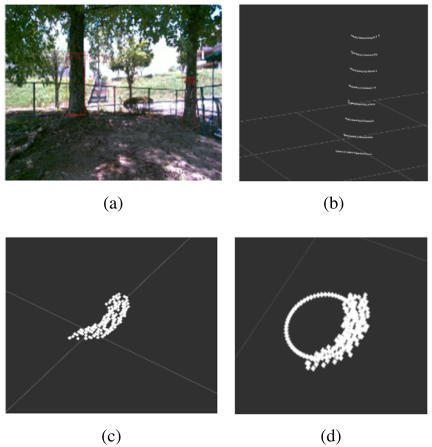
Fig. 3. Representative experimental example of incomplete LiDAR observations and resulting geometric estimation bias using LiDAR–RGB fusion.
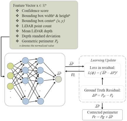
Fig. 4. Residual learning framework for geometric perimeter correction.
As illustrated in Fig. 4, the proposed framework takes observation-derived feature vector \(\boldsymbol{x}\) and geometric baseline estimates as input to a residual regression model that learns the systematic error associated with partial LiDAR observations. The predicted residual \(\widehat{\Delta P}\) is defined as Eq. \(\eqref{eq:9}\):
The final corrected perimeter is then obtained through additive refinement of the geometric baseline as defined in Eq. \(\eqref{eq:10}\).
The residual function \(f_{\phi}\) is implemented as a shallow multilayer perceptron with two hidden layers and ReLU activation functions. Given an input feature vector \(\boldsymbol{x}\), the network computes the correction as described by Eqs. \(\eqref{eq:11}\)–\(\eqref{eq:13}\).
To ensure generalization across different trees rather than memorization of tree-specific geometry, a tree-wise data split is employed: all frames associated with a given tree are assigned exclusively to either the training or testing set. This strategy prevents information leakage caused by temporal correlation among frames captured from the same tree. At inference time, the residual network operates as a lightweight post-processing module applied to each geometric perimeter estimate. Because the correction is additive and independent of the upstream perception pipeline, the model can be integrated without modifying the geometric reconstruction process, preserving modularity, interpretability, and computational efficiency while substantially reducing systematic bias in perimeter estimation.
Since multiple observations are available for each tree across consecutive frames, a sequence of corrected perimeter estimates \(P_{c}^{t}\), where \(t\) denotes the frame index, is obtained. To enhance temporal stability, filtering methods such as mean, median, exponential moving average (EMA), and Kalman filtering are applied to this sequence. For example, mean and median filters aggregate observations across frames to produce a stable estimate for each tree; EMA assigns higher weight to recent observations; and the Kalman filter recursively updates the estimate by accounting for measurement uncertainty. These filters reduce frame-to-frame variability and provide a robust final estimate for each tree, complementing the bias correction achieved by residual learning.
3. Experimental Setup and Data Collection
3.1. Experimental Platform, Environment, and Data Acquisition
Experiments were conducted using the mobile robotic platform in an outdoor forest environment. The experiments were conducted on the campus of Kyushu Institute of Technology, Iizuka, Japan, in a roadside forest-like environment. The study area consists of a narrow corridor along a campus road, with an effective sensing region of approximately 5 m in the lateral and forward directions relative to the robot trajectory. The vegetation is dominated by mixed deciduous tree species, including Sakura (cherry blossom), Ginkgo (Ginkgo biloba), and Japanese maple (Acer palmatum).
In total, approximately 100–125 trees were observed during data collection, with stem perimeters ranging from 25 cm to 160 cm, indicating low uniformity in the dataset. The samples include trees of varying sizes and spatial configurations, reflecting natural forest heterogeneity rather than controlled or uniform conditions. During robot traversal, only trees within the effective sensing range were included in the analysis.
Representative examples of the acquired sensor data are shown in Fig. 3, which are derived from actual field measurements and illustrate typical LiDAR–RGB observations under real environmental conditions. Cluttered backgrounds introduce practical sensing challenges, including incomplete LiDAR coverage, variable point density, and viewpoint-dependent visibility.
The robot navigated the environment using the ROS 2, and wheel encoder measurements fused with IMU data provided continuous odometry for motion control and temporal alignment of sensor streams. Importantly, odometry was used solely for navigation and synchronization and was not involved in geometric perimeter estimation or learning-based correction. During each run, the robot continuously acquired synchronized RGB images and 3D LiDAR point clouds. Tree stems were detected in the RGB images using a YOLO-based object detector YOLOv9, while the LiDAR sensor simultaneously captured the surrounding 3D structure. Using the extrinsic calibration between sensors, LiDAR points were associated with detected tree stems, enabling the extraction of stem-specific point clouds at each time step. As the robot approached and passed individual trees, multiple observations were recorded from different relative viewpoints, resulting in temporally correlated frame sequences for each tree.
3.2. Dataset Construction and Training Protocol
The dataset was constructed by pairing geometric perimeter estimates obtained from partial LiDAR observations with corresponding ground-truth measurements. For each detected tree stem and each frame, a geometric baseline perimeter \(P_g\) was computed using the procedure described in Section 2.2. Ground-truth perimeter measurements \(P_{gt}\) were obtained manually using a diameter tape at approximately DBH. Manual measurements were performed offline after data collection to avoid influencing robot motion or sensor readings.
The final dataset comprises approximately 1,450 frames collected from multiple distinct trees, with each tree contributing several frames captured under different viewpoints and occlusion conditions. The presence of multiple frames per tree introduces strong temporal correlation, which is explicitly considered during training and evaluation. For each frame, a feature vector \(\boldsymbol{x}\) was constructed from observation-derived descriptors and geometric reconstruction outputs as defined in Section 2.3.
The residual model is implemented as a shallow fully connected neural network with \(\mathit{ReLU}\) activation. It is trained using mean squared error loss and optimized with the Adam optimizer at a learning rate of \(1 \times 10^{-3}\). For temporal filtering, fixed parameters are used across all experiments to ensure consistent and unbiased comparison. The smoothing factor for EMA is \(\alpha = 0.3\), and for the Kalman filter, the initial estimate uncertainty is \(P = 0.01\), the process noise is \(Q=0.001\), and the measurement noise is \(R = 0.0025\).
To ensure generalization across unseen trees rather than memorization of tree-specific geometry, a tree-wise data split was employed. All frames associated with a given tree were assigned exclusively to either the training set or the testing set, preventing information leakage caused by repeated observations of the same stem. The residual neural network was trained by minimizing the mean squared error between predicted and true residuals using the training subset. During inference, the trained model operates as a post-processing module that independently refines each geometric baseline perimeter estimate. Performance evaluation compares baseline geometric estimates and residual-corrected estimates against ground-truth measurements on the held-out test set using standard regression metrics.
4. Results and Discussion
This section evaluates the effectiveness of the proposed residual learning framework for tree-stem perimeter estimation. Quantitative comparisons are conducted between the geometric baseline estimator and the residual-corrected model using a tree-wise held-out test set. The analysis focuses on overall accuracy improvement, error distribution characteristics, and robustness across varying stem sizes and sensing conditions.
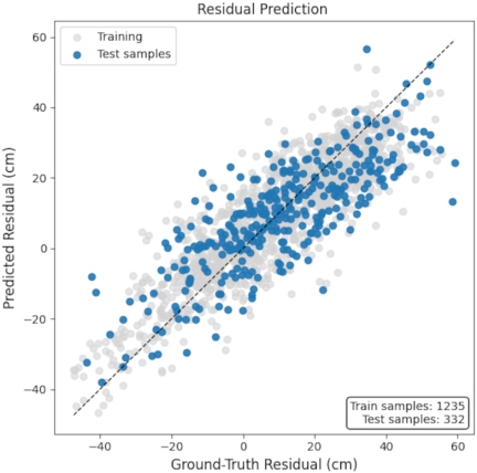
Fig. 5. Ground-truth residuals on tree-wise held-out test data.
To quantitatively assess performance, standard regression metrics are employed, including mean absolute error (MAE), root mean squared error (RMSE), mean relative error (MRE), and bias. MAE measures the average absolute deviation between estimated and ground-truth perimeters, while RMSE emphasizes larger errors through quadratic penalization. MRE provides a scale-normalized evaluation relative to ground-truth values, and bias represents the mean signed error, indicating systematic under- or over-estimation. Lower values of MAE, RMSE, and MRE indicate improved accuracy, while bias values closer to zero reflect reduced systematic error. While ground-truth perimeter measurements were obtained offline for evaluation purposes, the proposed correction model operates as a lightweight post-processing module and is suitable for real-time deployment on mobile forestry robots.
Figure 5 pictures the relationship between the predicted residuals and the ground-truth residuals of the geometric baseline for both training and tree-wise held-out test samples. Training samples (\(n = \textrm{1,235}\)) are shown in light gray for reference, while test samples (\(n = 332\)) are highlighted in blue. The dashed diagonal line represents the ideal one-to-one correspondence, indicating perfect residual prediction.
A strong linear alignment is observed across the full residual range (approximately \(-50\) cm to \(+60\) cm), demonstrating that the network accurately learns the magnitude and sign of the systematic error inherent in the geometric estimator rather than merely fitting local trends.
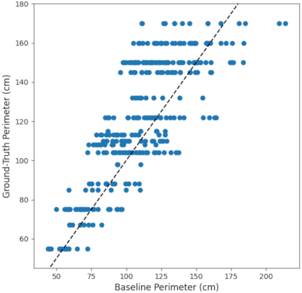
Fig. 6. Comparison between ground-truth and baseline perimeter estimates before residual correction.
The dense clustering of both training and test samples around the identity line confirms that the learned mapping generalizes well to unseen trees and does not exhibit noticeable overfitting or data leakage. Importantly, the dispersion remains approximately symmetric around the diagonal for positive and negative residuals, indicating consistent correction of both under-estimation and over-estimation regimes. Slightly increased spread at extreme residual magnitudes reflects higher uncertainty for highly occluded or sparsely observed stems, which is expected under realistic sensing conditions.
Figure 6 shows the relationship between the geometric baseline perimeter estimates and the corresponding ground-truth measurements for the tree-wise held-out test set. The dashed diagonal line indicates the ideal one-to-one correspondence.
A noticeable dispersion around the identity line is observed, particularly for medium and large stem perimeters. Many samples systematically deviate along the horizontal direction from the identity line, indicating persistent under- or over-estimation in the geometric baseline caused by incomplete LiDAR observations, occlusions, and deviations from ideal circular assumptions.
The presence of layered horizontal clusters reflects discretization effects (geometric ambiguity) introduced by incomplete LiDAR observations and limited angular coverage, where similar incomplete observations from different trees lead to similar fitted radii, producing repeated estimated perimeter values (horizontal alignment), which amplify geometric uncertainty under real forest sensing conditions. Although the baseline preserves a global linear trend, the increasing spread with perimeter magnitude highlights its sensitivity to incomplete observations and viewpoint variability, limiting its robustness for accurate stem sizing.
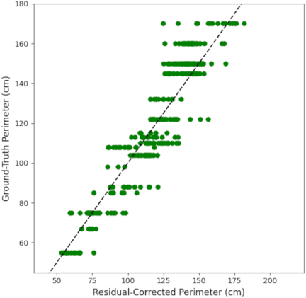
Fig. 7. Comparison between ground-truth and residual-corrected perimeter estimates.
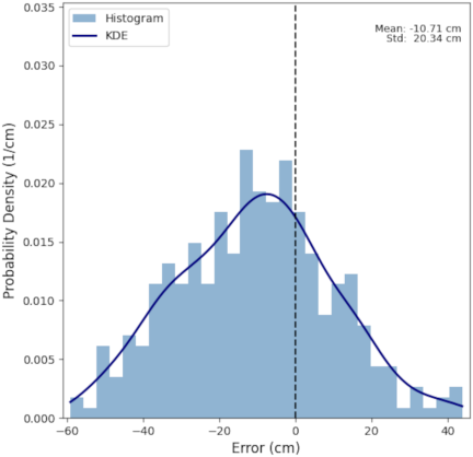
Fig. 8. Error distribution of geometric baseline perimeter estimates.
Figure 7 presents the corrected perimeter estimates after applying the proposed residual learning model. Compared with the geometric baseline, the corrected estimates exhibit a markedly tighter concentration around the identity line across the full perimeter range. Both under- and over-estimation regimes are substantially reduced, and the dispersion perpendicular to the diagonal decreases consistently for small and large stems.
The improved alignment indicates that the learned residual effectively compensates systematic geometric bias while preserving the monotonic relationship between estimated and measured perimeters. The reduction in clustering spread further demonstrates enhanced stability and consistency of the corrected estimates under varying sensing geometries.
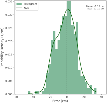
Fig. 9. Error distribution after residual learning correction.
Figure 8 illustrates the error distribution of the geometric baseline perimeter estimates. The error mean is shifted toward negative values (approximately \(-10.7\) cm), indicating a consistent systematic underestimation of stem perimeter. This bias arises primarily from partial arc visibility, occlusions, and uneven point density, which violate the assumptions of complete circular observations during geometric fitting. The relatively large standard deviation (approximately 20.3 cm) further indicates substantial dispersion and sensitivity to sensing conditions, including viewpoint variation and incomplete angular coverage. The broadened kernel density curve and long tails highlight unstable estimation behavior, especially under sparse or highly occluded observations.
Figure 9 presents the corrected error distribution after applying the proposed residual learning model. The mean error shifts close to zero (approximately \(-1.2\) cm), demonstrating effective compensation of the dominant systematic bias. Simultaneously, the standard deviation decreases to approximately 12.1 cm, reflecting a substantial reduction in estimation variability and improved consistency across samples. The kernel density curve becomes sharper and more symmetric around zero, indicating that the correction reduces both bias and dispersion rather than merely suppressing random noise. Importantly, the absence of saturation or clipping effects suggests that the learned correction remains stable across the full error range.
The contrast between Figs. 8 and 9 confirms that residual learning transforms a biased and widely dispersed error distribution into a compact and near-zero-centered distribution. This behavior validates that the model captures structured geometric distortion patterns caused by partial arc observations rather than overfitting to individual samples.
Table 1. Performance comparison between geometric baseline and proposed residual correction model.

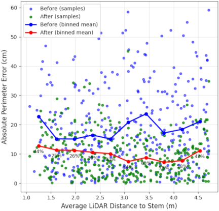
Fig. 10. Absolute perimeter error versus LiDAR sensing distance before and after residual correction.
As summarized in Table 1, the geometric baseline yields an MAE of 18.42 cm and an RMSE of 22.99 cm, with a coefficient of determination \(R^{2} = 0.480\), reflecting limited predictive accuracy under partial arc observations. After residual learning correction, MAE decreases to 9.67 cm and RMSE to 12.16 cm, corresponding to relative reductions of 47.5% and 47.1%, respectively. The goodness of fit improves substantially to \(R^{2} = 0.855\), representing an absolute increase of 0.374. In relative terms, the average percentage error decreases from 14.79% to 8.30%, confirming a consistent reduction in systematic bias.
Figure 10 illustrates the relationship between absolute perimeter estimation error and mean LiDAR sensing distance for both the geometric baseline and the proposed residual learning model. Individual samples are shown as scattered points, while solid curves represent binned MAEs across depth intervals. Annotated percentages indicate relative error reduction compared to the baseline within each distance bin. The geometric baseline exhibits consistently higher errors across all distance ranges, with binned mean errors typically varying between approximately 15–24 cm. Error magnitudes increase noticeably at medium and farther ranges, reflecting the compounded effects of reduced point density, limited angular coverage, and partial arc visibility, which amplify geometric bias under long-range sensing conditions. In contrast, the proposed residual learning model maintains substantially lower binned mean errors, remaining largely below 8–12 cm across the full depth range. The annotated relative improvements range from approximately 25% at near distances to over 60% at medium-to-far ranges, where partial arc effects are most pronounced. This trend demonstrates that the correction model effectively compensates for range-dependent geometric distortion and generalizes robustly across sensing distances.
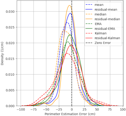
Fig. 11. Error distribution comparison of filtering methods (dashed) and residual-corrected methods (solid).
It is important to note that the Velodyne VLP-16 LiDAR provides a typical ranging accuracy of approximately \(\pm 3\) cm up to 100 m. However, in this study, the effective sensing region was limited to approximately 5 m to ensure sufficient point density and reliable stem observations. The improved alignment observed in the absolute error trends and error distributions is consistent with the quantitative gains reported in Table 1, including a 47.5% reduction in MAE and a 47.1% reduction in RMSE, and a substantial increase in the coefficient of determination from \(R^{2} = 0.48\) to \(R^{2} = 0.85\). Together, these results confirm that residual learning significantly improves absolute perimeter estimation accuracy while preserving the interpretability and structural consistency of the geometric baseline.
To further evaluate the robustness of the proposed residual learning framework across different temporal (time-based, using multiple observations of the same object over time) strategies, an additional analysis is conducted by integrating residual correction with multiple filtering methods. As shown in Fig. 11, baseline filtering methods exhibit a noticeable leftward shift, indicating persistent underestimation bias.
Dashed curves represent baseline filtering methods, while solid curves correspond to residual-corrected estimates, where labels such as “residual-mean,” “residual-median,” “residual-EMA,” and “residual-Kalman” indicate that the corresponding temporal filter is applied to the residual-corrected perimeter estimates.
Table 2. Quantitative performance comparison of baseline filtering and residual-corrected filtering methods.

After applying residual learning, all distributions shift toward the zero-error line and become more symmetric, confirming consistent reduction of systematic bias across filtering strategies. Among the evaluated methods, the residual median produces the most compact and well-centered distribution, indicating superior stability and bias correction. Residual mean also shows strong improvement, whereas EMA and Kalman filtering retain relatively wider spreads, suggesting higher sensitivity to temporal variability.
The distributional improvements are further supported by the quantitative results in Table 2. Residual learning consistently reduces error metrics across all filtering methods, with the most pronounced improvement observed for the median-based approach.
Negative bias values indicate systematic underestimation of perimeter, while values closer to zero reflect reduced systematic error. In particular, the residual median achieves the best overall performance, with the lowest MAE (9.60 cm), RMSE (12.60 cm), and bias (\(-3.26\) cm), indicating effective reduction of both estimation error and systematic underestimation. Similar improvements are observed for the residual mean and residual EMA, while the residual Kalman method shows comparatively moderate gains. These results confirm that residual learning enhances the accuracy and consistency of perimeter estimation across different temporal filtering strategies.
Beyond numerical improvements, it is important to interpret how these gains arise from the structural design of the proposed model. Rather than replacing the geometric estimator, the residual network is explicitly formulated to learn only the systematic discrepancy between geometric predictions and ground-truth measurements. This design ensures that the correction remains bounded, physically meaningful, and interpretable—an important requirement for robotic perception systems operating in safety-critical and resource-constrained environments. This effect is consistently observed in the error distribution comparisons (Fig. 11), where all methods exhibit a shift toward the zero-error line after residual correction, as well as in the quantitative improvements summarized in Table 2.
On the other hand, the contraction of error distributions observed after correction reflects the model’s ability to capture recurring geometric biases caused by partial stem visibility, irregular point density, and viewpoint-dependent arc formation. Because the residual is learned directly in the perimeter domain, the network implicitly encodes how incomplete circular arcs distort perimeter estimation without requiring explicit modeling of stem shape variability or occlusion geometry.
The distance-wise stability of the corrected estimates further supports this interpretation. The residual model does not directly depend on absolute range but instead leverages normalized geometric and semantic features derived from the LiDAR–RGB fusion stage. As a result, the correction generalizes across varying sensing distances and stem sizes, indicating that the model learns scale-consistent error patterns rather than depth-specific adjustments. Furthermore, the consistent reduction in MAE and bias across all filtering strategies (Table 2) demonstrates that the residual correction complements temporal filtering by improving both accuracy and robustness.
The strong linear alignment between predicted and ground-truth residuals confirms that the correction operates in a near-linear regime, consistent with the lightweight architecture of the network and its role as a structured bias compensator rather than a high-capacity regressor. Retaining the geometric estimator ensures physical interpretability, while the residual model focuses only on correcting systematic deviations rather than replacing the underlying structure. This behavior mitigates overfitting and enables reliable generalization across unseen trees, as ensured by the tree-wise data split strategy.
From a systems perspective, the residual model’s role as a post-processing module enables seamless integration into the overall mapping pipeline. Since geometric estimation remains the primary source of structural information, the corrected perimeter estimates retain physical interpretability and can be directly propagated to downstream localization, mapping, and inventory components. The modular design further allows the correction model to be retrained or updated independently as new data become available, supporting long-term deployment in evolving forest environments.
5. Conclusion
This paper presented a LiDAR–RGB fusion–based framework for robust tree-stem perimeter estimation in forest environments, addressing the inherent limitations of geometric methods, where estimation error is dominated by systematic bias under partial visibility and sparse sensing conditions. While geometric circle fitting provides an interpretable baseline, its accuracy degrades substantially when observations are incomplete or unevenly distributed, a common condition in real-world forestry scenarios. To overcome this limitation, a residual learning strategy was introduced to compensate for systematic geometric bias without discarding the physical structure of the baseline estimator. By learning the discrepancy between geometric perimeter estimates and ground-truth measurements, the proposed model operates as a lightweight post-processing module that refines each estimate independently while preserving interpretability.
Extensive experimental evaluation using a tree-wise held-out protocol demonstrates that the proposed approach consistently reduces both systematic bias and estimation variance, leading to improved accuracy and consistency. The corrected estimates exhibit reduced bias, tighter error distributions, improved goodness-of-fit, and stable performance across varying stem sizes and sensing distances. Importantly, these gains are achieved without increasing model complexity or introducing range-dependent heuristics, highlighting residual learning as a useful enhancement to geometric estimation.
Furthermore, integrating temporal filtering over multiple observations demonstrates that filtering alone reduces variability but cannot eliminate systematic bias, whereas the combination with residual learning achieves both bias correction and temporal stability. From a system integration perspective, the modular design of the correction model enables seamless deployment on mobile forestry robots, where computational efficiency and robustness are critical. Because the correction operates as a lightweight post-processing step, it can be executed onboard in real time and integrated directly into existing perception and mapping pipelines without modifying core navigation or localization components. The framework supports continuous mapping and can be readily extended to larger-scale environments or incrementally updated as additional data become available.
Future work will explore extending the residual correction framework to jointly model stem shape irregularities, incorporating temporal consistency across repeated observations, and validating performance in denser forest environments with higher occlusion levels. Integrating uncertainty-aware residual prediction into global tree mapping and inventory systems also remains an important direction for further research.
- [1] L. Deng, M. Fujio, X. Lin, and R. Ota, “Labor shortage and early robotization in Japan,” Econ. Lett., Vol.233, Article No.111404, 2023. https://doi.org/10.1016/j.econlet.2023.111404
- [2] H. Gupta, H. Andreasson, A. J. Lilienthal, and P. Kurtser, “Robust scan registration for navigation in forest environment using low-resolution LiDAR sensors,” Sensors, Vol.23, No.10, Article No.4736, 2023. https://doi.org/10.3390/s23104736
- [3] Y. Sheng, Q. Zhao, X. Wang, Y. Liu, and X. Yin, “Tree diameter at breast height extraction based on mobile laser scanning point cloud,” Forests, Vol.15, No.4, Article No.590, 2024. https://doi.org/10.3390/f15040590
- [4] D. Tiozzo Fasiolo, L. Scalera, E. Maset, and A. Gasparetto, “Field evaluation of an autonomous mobile robot for navigation and mapping in forest,” Robotics, Vol.14, No.7, Article No.89, 2025. https://doi.org/10.3390/robotics14070089
- [5] T. Ota et al., “Estimating aboveground carbon using airborne LiDAR in Cambodian tropical seasonal forests for REDD+ implementation,” J. For. Res., Vol.20, No.6, pp. 484-492, 2015. https://doi.org/10.1007/s10310-015-0504-3
- [6] J. Gonzalez de Tanago et al., “Estimation of above-ground biomass of large tropical trees with terrestrial LiDAR,” Methods Ecol. Evol., Vol.9, No.2, pp. 223-234, 2018. https://doi.org/10.1111/2041-210X.12904
- [7] G. Fan, L. Nan, Y. Dong, X. Su, and F. Chen, “AdQSM: A new method for estimating above-ground biomass from TLS point clouds,” Remote Sens., Vol.12, No.18, Article No.3089, 2020. https://doi.org/10.3390/RS12183089
- [8] L. Xu et al., “Forest aboveground biomass estimation based on spaceborne LiDAR combining machine learning model and geostatistical method,” Front. Plant Sci., Vol.15, Article No.1428268, 2024. https://doi.org/10.3389/fpls.2024.1428268
- [9] Z. M. Bhebhe, X. Liu, Z. Zhang, and D. R. Paudyal, “Estimation of tree diameter at breast height (DBH) and biomass from allometric models using LiDAR data: A case of the Lake Broadwater Forest in Southeast Queensland, Australia,” Remote Sens., Vol.17, No.14, Article No.2523, 2025. https://doi.org/10.3390/rs17142523
- [10] A. Bornand, N. Rehush, F. Morsdorf, E. Thürig, and M. Abegg, “Individual tree volume estimation with terrestrial laser scanning: Evaluating reconstructive and allometric approaches,” Agric. For. Meteorol., Vol.341, Article No.109654, 2023. https://doi.org/10.16904/envid
- [11] Y. Wu, S. Zhong, Y. Ma, Y. Zhang, and M. Liu, “Application of SLAM-based mobile laser scanning in forest inventory: Methods, progress, challenges, and perspectives,” Forests, Vol.16, No.6, Article No.920, 2025. https://doi.org/10.3390/f16060920
- [12] S. Ma, Y. Chen, Z. Li, J. Chen, and X. Zhong, “Improved cylinder-based tree trunk detection in LiDAR point clouds for forestry applications,” Sensors, Vol.25, No.3, Article No.714, 2025. https://doi.org/10.3390/s25030714
- [13] T. P. Pitkänen, P. Raumonen, and A. Kangas, “Measuring stem diameters with TLS in boreal forests by complementary fitting procedure,” ISPRS J. Photogramm. Remote Sens., Vol.147, pp. 294-306, 2019. https://doi.org/10.1016/j.isprsjprs.2018.11.027
- [14] S. C. Florea, I. Dutcă, and M.-D. Niță, “Tradeoffs and limitations in determining tree characteristics using 3D pointclouds from terrestrial laser scanning: A comparison of reconstruction algorithms on European bech (Fagus sylvatica L.) trees,” Ann. For. Res., Vol.67, No.2, pp. 185-199, 2024. https://doi.org/10.15287/afr.2024.3885
- [15] X. Liang et al., “Close-range remote sensing of forests: The state of the art, challenges, and opportunities for systems and data acquisitions,” IEEE Geosci. Remote Sens. Mag., Vol.10, No.3, pp. 32-71, 2022. https://doi.org/10.1109/MGRS.2022.3168135
- [16] M. Mokroš et al., “Evaluation of close-range photogrammetry image collection methods for estimating tree diameters,” ISPRS Int. J. Geo-Inf., Vol.7, No.3, Article No.93, 2018. https://doi.org/10.3390/ijgi7030093
- [17] R. Fekry, W. Yao, L. Cao, and X. Shen, “Ground-based/UAV-LiDAR data fusion for quantitative structure modeling and tree parameter retrieval in subtropical planted forest,” For. Ecosyst., Vol.9, Article No.100065, 2022. https://doi.org/10.1016/j.fecs.2022.100065
- [18] P. Wan et al., “Quantification of occlusions influencing the tree stem curve retrieving from single-scan terrestrial laser scanning data,” For. Ecosyst., Vol.6, Article No.43, 2019. https://doi.org/10.1186/s40663-019-0203-1
- [19] A. Nurunnabi, F. Teferle, A. Novo, J. Balado, and E. Ientilucci, “Derivation of tree stem curve and volume using point clouds,” Int. Arch. Photogramm. Remote Sens. Spat. Inf. Sci., Vol.XLVIII-4/W11-2024, pp. 81-88, 2024. https://doi.org/10.5194/isprs-archives-XLVIII-4-W11-2024-81-2024
- [20] S. Macenski, T. Foote, B. Gerkey, C. Lalancette, and W. Woodall, “Robot operating system 2: Design, architecture, and uses in the wild,” Sci. Robot., Vol.7, No.66, Article No.eabm6074, 2022. https://doi.org/10.1126/scirobotics.abm6074
- [21] T. Diwan, G. Anirudh, and J. V. Tembhurne, “Object detection using YOLO: Challenges, architectural successors, datasets and applications,” Multimed. Tools Appl., Vol.82, No.6, pp. 9243-9275, 2023. https://doi.org/10.1007/s11042-022-13644-y
- [22] A. A. Murat and M. S. Kiran, “A comprehensive review on YOLO versions for object detection,” Eng. Sci. Technol. Int. J., Vol.70, Article No.102161, 2025. https://doi.org/10.1016/j.jestch.2025.102161
- [23] M. L. Ali and Z. Zhang, “The YOLO framework: A comprehensive review of evolution, applications, and benchmarks in object detection,” Computers, Vol.13, No.12, Article No.336, 2024. https://doi.org/10.3390/computers13120336
- [24] K. Levenberg, “A method for the solution of certain non-linear problems in least squares,” Q. Appl. Math., Vol.2, No.2, pp. 164-168, 1944. https://doi.org/10.1090/qam/10666
- [25] D. W. Marquardt, “An algorithm for least-squares estimation of nonlinear parameters,” J. Soc. Ind. Appl. Math., Vol.11, No.2, pp. 431-441, 1963. https://doi.org/10.1137/0111030
This article is published under a Creative Commons Attribution-NoDerivatives 4.0 Internationa License.