Research Paper:
Efficient Method to Create 3D Models Based on Center Lines and Cross-Sectional Geometries from Point Cloud of an Entire Steel Truss Bridge
Nao Hidaka†, Daisuke Uchiyama, and Ei Watanabe
Nagoya Institute of Technology
Gokiso-cho, Showa-ku, Nagoya, Aichi 466-8555, Japan
†Corresponding author

For efficient maintenance of existing bridges, quantitative evaluation of residual load capacity using numerical analysis with FE models is widely adopted. Among various FE models, the fiber-based model, composed of center lines and cross-sectional geometries, is particularly effective for analyzing entire bridges. However, as-built drawings are often unavailable, and bridge conditions inevitably change over time, necessitating modeling methods that do not rely on design drawings. Point cloud data, capable of capturing as-is 3D geometry, have therefore attracted increasing attention. The authors have previously developed a method to semi-automatically construct fiber-based models from point clouds of entire steel truss bridges. However, a mismatch remains between the dimensional reproducibility required for load-bearing capacity analysis and the limitations imposed by measurement equipment and site conditions. While millimeter-level accuracy is required, measurement conditions are often constrained, resulting in incomplete or low-quality data. To address this issue, this study proposes an extended method incorporating deep learning. A measurement simulation tool is introduced to generate training data that reflect realistic laser scanner conditions, improving member recognition accuracy even in regions with poor measurement quality. Furthermore, deep learning enables the estimation of flange and web dimensions as well as plate thickness. As a result, the proposed method improves dimensional reproducibility and represents a step forward in capturing the overall structural configuration of entire bridges.
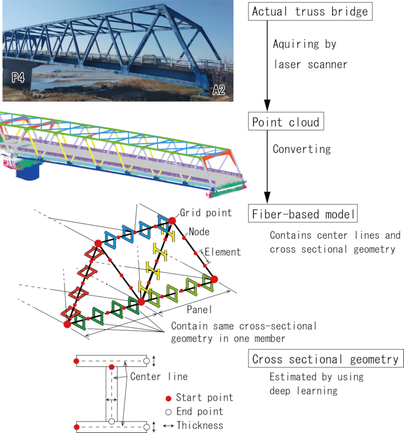
Creating a fiber-based model from point cloud
1. Introduction
A vast number of existing bridges are rapidly aging. Since it is not practical to rebuild all of them at the same time, strategic renewal through life cycle extension is required. To support this, quantitative evaluation of residual load capacity using numerical analysis is increasingly adopted with high reproducibility achieved by FE models validated through structural experiments 1. The FE models can be classified into several types, as shown in Fig. 1. For entire bridges design under strong earthquake and considering convenience in numerical analysis, fiber-based models composed of a center line and cross-sectional geometries are desirable.
However, efficiency of the generation method remains an issue. Construction of an FE model requires acquisition of member dimensions of a target structure. However, in cases of old bridges, as-build drawings are often unavailable. In addition, condition of bridges has inevitably changed since their construction due to various factors. Therefore, it is necessary to construct an FE model without relying on drawings, but manual measurement is time-consuming and prone to various human errors.
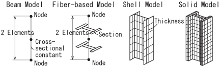
Fig. 1. The types of FE models used in structural mechanics.
Therefore, point cloud data, capable of capturing as-is 3D geometry as a set of points quickly and widely, have begun to attract attention. Nowadays, various types of FE modeling have been attempted for point clouds of bridge members. While there are examples of converting point cloud data into shell models 2 or solid models 3 based on converting surface geometry, these approaches have the limitation of not covering the entire bridge. On the other hand, Hidaka et al. 4 developed the method to semi-automatically construct fiber-based models from point clouds of an entire steel truss bridge. However, the mismatch between the reproducibility accuracy in load-bearing capacity analysis of steel structures and the measurement equipment and site constraints remained as issue. Steel bridges require millimeter-level reproducibility, but due to the distribution of section forces, even identical members may have varying flange and web lengths or plate thicknesses. Furthermore, measurement site constraints can result in areas that cannot be measured or where measurement quality is poor. As a result, only some members could be measured in detail, leaving issues regarding the model’s reproducibility. In addition, it is required to recognize and segment members from entire bridge point cloud, but in the past research 4, members were set manually. Therefore, as a follow-up, we proposed a segmentation method utilizing deep learning 5. However, since the training data was generated by sampling pseudo points on the surface of 3D CAD models, there remains an issue of discrepancies with actual laser measurements.
Based on the above, this paper expands upon the previous research 4,5, developing efficient fiber modeling techniques while considering entire steel truss bridges and the characteristics of point cloud measurement data. By utilizing deep learning, we have developed a method for determining the length and thickness of flanges and webs from point cloud data generated by stationary laser scanners, which offer moderate measurement accuracy but can cover a wide area. Furthermore, by generating training data using a pseudo-point cloud measurement tool, we aim to improve the accuracy of member segmentation.
2. Point Cloud Measurement
2.1. Case Study of the Bridge
The case study is through-type steel truss bridge in Aichi Prefecture, Japan. It consists of two-span and three-span continuous bridge. Each span contains seven panels. A photograph of the bridge is shown in Fig. 2. A side view drawing of the entire bridge is shown in Fig. 3, and a detailed side view drawing for a single span is shown in Fig. 4. Cross-sectional views are shown in Fig. 5. “A1” and “A2” shown in Figs. 3 and 4 correspond to abutments supporting the ends of the bridge, while “P1,” “P2,” and “P3” are piers supporting the middle section. The symbols used in the figures and tables that follow refer to the same items. In addition, the members vary in flange and web length and plate thickness according to the distribution of section forces. Tables 1–6 summarize the lengths and plate thicknesses of the flanges and webs for each member in the P4-A2 span and A1-P1 span. The dimensions described in the left figure of each table are not varied in panels. This bridge is a river crossing bridge, and access to the space beneath the girders is restricted to within approximately 45 meters of abutment A2.
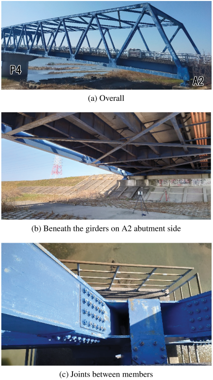
Fig. 2. Photographs of the case study bridge.
2.2. Measurement Instruments
In this research, two types of laser scanners were used. Due to site constraints, measurements were taken only for span P4-A2. As a supplementary note, regarding the use of drones, since the bridge is currently in use, measurements must be taken from 30 m. Consequently, it is unsuitable for shape reconstruction via photogrammetry and is therefore not being utilized.
2.2.1. Stationary Laser Scanner
Leica RTC360 (resolution: 3 mm at 10 m, accuracy: 1.9 mm at 10 m) was used. This is mounted on a tripod to measure point clouds in all directions. Basically, measurements are taken at multiple points and then integrated. Each measurement takes one to two minutes.
2.2.2. Handheld Laser Scanner
HandySCAN BLACK™ Elite (resolution: 0.05 mm at 30 cm, accuracy: 0.025 mm at 30 cm) was used. This is measured by holding it in hand and moving it. To estimate the device’s own position, markers must be attached beforehand at approximately 5 cm intervals. Therefore, each measurement takes about 30 minutes.
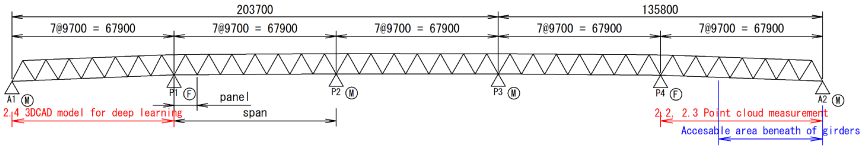
Fig. 3. Side view drawing of the case study bridge.
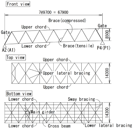
Fig. 4. Detailed drawing for a single span side view.
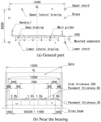
Fig. 5. Cross sectional views.
Table 1. Cross-sectional geometries of the upper chords (based on the drawings).

Table 2. Cross-sectional geometries of the lower chords (based on the drawings).

2.3. Measurement Results
A summary of the measurement results is shown in Fig. 6. We measured the entire P4-A2 span using a stationary laser scanner and measured portions of the structure using a handheld laser scanner.
Table 3. Cross-sectional geometries of the compressed braces (based on the drawings).

Table 4. Cross-sectional geometries of the tensile braces (based on the drawings).

Table 5. Cross-sectional geometries of the main girders and the cross beams (based on the drawings).

Table 6. Cross-sectional geometries of the upper and lower lateral bracings (based on the drawings).

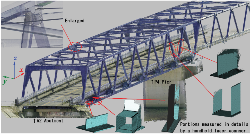
Fig. 6. A summary of the measurement results.
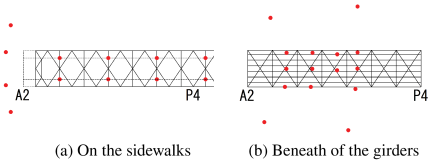
Fig. 7. Measurement locations by using the stationary laser scanner (red points).
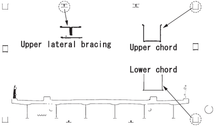
Fig. 8. Cross section of the measured point cloud by using the stationary laser scanner.
2.3.1. Stationary Laser Scanner
As shown in Fig. 7, point cloud measurements were taken from 12 locations on the sidewalk and 15 locations beneath the girders, and these were integrated. The total point was 1,065,353,413. The upper surfaces of the upper chords, lower chords, and upper lateral bracings were not measured as the laser was not hit at them (Fig. 8). Also, the laser scanner could not be placed beneath the girders in panels 1, 6, and 7, resulting in poor measurement quality for the components below the slab (Fig. 9).
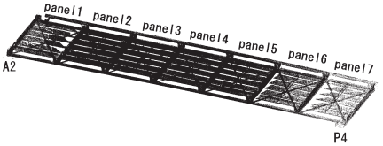
Fig. 9. The measured point cloud under the slab.
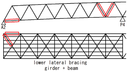
Fig. 10. The measurement places by using the handheld laser scanner.
2.3.2. Handheld Laser Scanner
Only a portion of the member accessible from beneath the girders or the sidewalk could be measured. Although it was possible to measure all brace members from the sidewalk, only two members were measured as representatives due to time constraints. They are expected to be subjected significant sectional forces. D12 and D13 correspond within the P4-A2 span, as shown in Tables 3 and 4. Only limited portions of the lower chord, lower lateral bracing, and main girders near the A2 abutment bearing seat, which were within reach from the bearing seat surface, could be measured. Fig. 10 shows the measurement places. Since the laser measurements were conducted from the sidewalk, only the brace members on one side of the bridge could be scanned (Fig. 11).
2.4. Creating Training Data from 3D CAD Model
Point cloud data for deep learning training were synthetically generated from 3D CAD models in A1-P1 span based on the drawings. The tool to generate pseudo point cloud is Helios\(\texttt{++}\) 6. The measurement conditions replicated the Leica RTC360’s measurement accuracy and resolution, and the measurement position was the same as in Fig. 7. The points have only one label for the corresponding members (Fig. 12), such as Fig. 13.
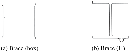
Fig. 11. Cross section of the measured point cloud by using by using the handheld laser scanner.
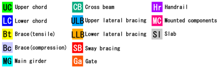
Fig. 12. The labels of the member.
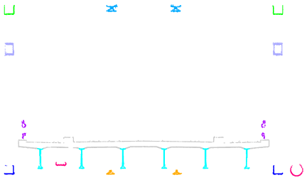
Fig. 13. The example of training data for deep learning (colors are corresponded to the label in Fig. 12).
3. Method to Construct a Fiber-Based Model of a Steel Truss Bridge from Point Clouds
3.1. Requirements of the Fiber-Based Model
This section describes the configuration of the fiber-based model developed in this research and the approach used to extract the requirements from point cloud data. A center line consists of elements connecting two nodes that define coordinates. Each element is associated with a cross-sectional geometry. It is defined as multiple rectangles as shown in Fig. 14. Each rectangle is defined by the coordinates of its starting and ending points and the plate thickness. The 3D shape is created by sweeping a cross-section within an element. The connection of members is achieved by sharing end nodes, and these nodes are defined as “grid points.”
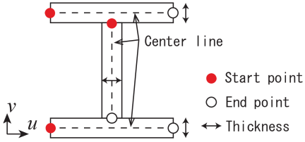
Fig. 14. Parameters of section for fiber-based model.
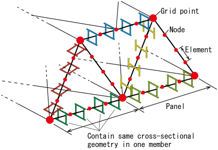
Fig. 15. The fiber-based model structure used in this research.
Although it is ideal to detect cross-sectional geometry in each element by using the surrounding point cloud, this is not yet practical due to noise and missing data. Therefore, this research prioritizes capturing the overall shape from the point cloud data of the entire bridge, defining a representative cross-sectional shape for each individual member composed of multiple elements. This method utilizes the geometric characteristic that bridge members have swept-section shapes, offering the advantage of compensating for missing points in the point cloud based on the author’s past method 7. Note that at the connection points of members, the plate thickness locally increases due to overlapping plates; however, this research ignores these points and applies the plate thickness outside the connection areas.
Figure 15 shows the fiber-based model structure used in this research, exemplified by a two-panel truss bridge.
3.2. Overview of the Proposed Method
The proposed method consists of three main steps. First, single members are recognized and segmented from entire bridge. Second, a center line for each member is created. Third, lengths and thickness of flanges and webs of each member are detected. Other requirements such as materials, boundaries, and loadings are not described in this paper.
3.3. Segmentation Members from Point Cloud
Common segmentation methods for point clouds involve dividing points based on thresholds such as coordinates or colors, as well as applying techniques such as RANSAC 8 or region growing 9 to fit lines or planes. These processes require the appropriate setting of thresholds. In general, it is not easy to set the threshold dynamically in automatic processing because of the effects of point density, missing points, and other factors. In recent years, deep learning has attracted attention as a method for dynamically setting threshold values, and there are several cases where it has been applied to point cloud data processing. However, when targeting large-scale bridges with a wide variety of geometries, the classification is roughly divided into upper and lower structures, and the lack of training data and the number of input points are insufficient. Therefore, the authors 5 focused on the characteristics of bridges, which generally have many structures with swept cross sections of each member along a longitudinal direction, and the fact that classification methods for 2D images are relatively well-developed. So, point cloud data of 2D cross sections sliced along the longitudinal direction as shown in Fig. 13 are used to classify members using deep learning. The method for acquiring cross-sectional point cloud is described in detail in Section 3.4. By inputting point cloud data of cross sections, the number of input points can be reduced, and the number of training data can be increased.
Table 7. Parameters of deep learning.

In this research, the training model under the conditions that yielded the highest segmentation accuracy based on past results 5 is adopted. First, PointNet\(\texttt{++}\) 10 is used. Next, the preprocessing methods for input data are described. Cross-sectional point clouds without normal vectors are randomly sampled to reduce the number of input points for deep learning to 6,164. To normalize the scale, adjust the origin to the midpoint between the minimum and maximum values of the \(XY\) coordinates, and scale the points so that the distance from the origin to the farthest point equals 1. Finally, in classification models, there are cases where weights for loss are adjusted to prevent bias in recognizing data with few labels; however, in this research, the weight for all labels was set to 1. Other general parameters related to deep learning are as shown in Table 7.
As described in Section 2.4, the method for acquiring the point cloud of the training data from 3DCAD is updated. The reason is that pseudo-sampling points from the surface of 3D CAD models include points of inside components not hit by the laser.
The results of segmentation are reused as cross-sectional point clouds in Sections 3.5.2 and 3.6.
3.4. Creating Cross-Sectional Point Cloud Data
A cutting plane is defined and points whose distance from the plane is less than or equal to \(d\) are projected onto the plane (Fig. 16). \(d\) is an arbitrary value. Furthermore, the point clouds are applied by an affine transformation to local coordinates on the cut surface for converting 2D point clouds.
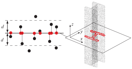
Fig. 16. The method to create cross-sectional point cloud.
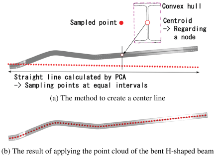
Fig. 17. The method to create cross-sectional point cloud.
3.5. Creating Center Lines from Point Cloud Data
3.5.1. For a Single Member
To accurately reflect component curvature, the center line is generated as a 3D polyline rather than a single straight line. To create a polyline, the centroid of a point cloud of a cross-section is used. However, since using a centroid of a point cloud is affected by noise, missing data, and density variations, it is calculated after converting 2D polygon by using convex hull. Since cross-sections of bridge components are symmetrical, even when cutting the cross-section diagonally, the centroid can be obtained at the center.
The result of applying the point cloud of bent H-shaped beam is shown in Fig. 17. At first, a line is defined consisting of the centroid of the point cloud and the first principal component vector obtained by principal component analysis. This is the result of obtaining the centroids by setting vertical cross-sections at equal intervals along the line from its starting point to its end point and then obtaining point clouds from each cross-section.
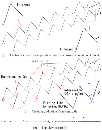
Fig. 18. Creating grid points from centroids of the braces and segmentation each panel.
3.5.2. For Multiple Members
As a preprocessing step, groups of points on the member are segmented from the cross-sectional point cloud by using the method described in Section 3.3. Furthermore, the points of each member can be applied to the method described in Section 3.5.1 to determine the centroids. As a result, candidate points for the center line of each member are generated. Fig. 18(a) shows the result of obtaining the centroids of braces as an example. Next, adjacent grid points are used to divide them into a single unit. The cross-sectional shape varies locally near the connection point due to multiple overlapping plates, causing the centroids to deviate from the center line of the single member. This affects the coordinate shift of the grid points. Therefore, we estimated straight lines using RANSAC from a set of centroids avoiding the around the connection points and determined the grid points from the intersection of adjacent straight lines (Fig. 18(b)). The grid points of braces are adopted as representative. The reason is that braces connect to most other members and have a characteristic where the center lines of adjacent members are oriented diagonally and their \(Z\)-directions are reversed. Also, in the process of creating the center lines to a polyline, only the set of centroids avoiding around of the connection points is used.
3.6. Detecting Cross-Sectional Geometries from Point Cloud Data
The authors proposed a method for automatically extracting the cross-sectional geometries of fiber-based models such as length and thickness of flanges and webs from point cloud data of cross-sections 4. First, we explain this in Sections 3.6.1 and 3.6.2. However, this method can only be applied to point clouds that have noise removed, are free of missing data, and exhibit minimal dispersion due to measurement errors. In the context of this research’s case, point cloud measured in detail across the entire surface of members using the handheld laser scanner is applicable, but point cloud data measured using the stationary laser scanner are not suitable. To handle lower quality point clouds, we developed a method to predict necessary parameters using PointNet\(\texttt{++}\) 10. This is explained in Section 3.6.3.
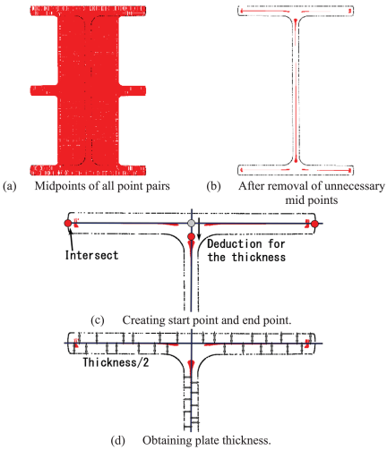
Fig. 19. Getting parameters of close-cross section.
3.6.1. Open Cross-Section (I-Shape and T-Shape)
As shown in Fig. 14, cross-sectional geometries can be acquired if the center lines of its rectangles are detected. To detect the center lines, it is effective using the method based on the symmetry detection from geometric models 7. In other words, it is possible to detect candidate points of the center lines by creating midpoints of pair points in the point cloud of the cross section. While midpoints of all point pairs (Fig. 19(a)) contain points that are not correspond to the center lines, the midpoints of the pairs whose distances are over general plate thickness and the midpoints on the point cloud of the cross section are removed. The detected midpoints are shown as Fig. 19(b). The points are converted to straight lines as the center lines by using RANSAC. The start and end point are created as interpoints of the center lines and the point cloud of the cross section (Fig. 19(c)). The plate thickness is obtained by doubling an average of the shortest distances from the cross-sectional point cloud (Fig. 19(d)).
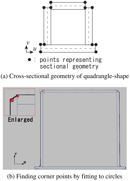
Fig. 20. Getting parameters of close-cross section.
3.6.2. Close Cross-Section (Quadrangle-Shape)
The algorithm in Section 3.6.1 cannot be applied to a quadrangle-shape cross section because back sides of plates cannot be measured. Therefore, as shown in Fig. 20(a), cross-sectional geometry is constructed by finding points at corners. Since corner points and joint positions are rounded, as shown in Fig. 20(b), corner points can be found by taking a local area at all points of the cross section and extracting the area where the radius of the circle is smaller when fitting it to a circle. For areas where thickness cannot be measured, such as the web and the upper flange of the lower chord, general plate thicknesses are used.
3.6.3. Estimation Using Deep Learning
The predicted values are the length and plate thickness of the flanges and the webs. Under the premise that the shapes of truss members are limited, the training model is created for each type of member.
The cross-sectional point cloud, segmented using the method described in Section 3.3 and containing only points labeled with the specified member, is used as the input data. This paper focuses on the “upper chords,” “lower chords,” “braces,” and “lower lateral bracings" that sweep along the longitudinal direction and exhibit varying cross-sectional dimensions. Since the length and plate thickness differ by nearly a factor of ten, we apply weighting to the plate thickness during loss function calculation. Note that some cross-sectional point clouds sliced along the longitudinal direction are not perpendicular to the members. However, as the training and validation data exhibit similar trends in this research, these data are directly used as input without modification. Since the flange and web lengths and plate thicknesses of truss bridges vary for each single member, the predicting result was the average of the predicted values obtained when inputting the cross-sectional point clouds of each single member. Fig. 21 shows the result of verification by using training data.
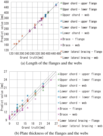
Fig. 21. Validation of predict cross-sectional geometries by using training data.
4. Results and Discussions
4.1. Overview
To verify the effectiveness of the proposed method, we compare the results of the three main step approaches with past results. The implementation environment is as shown in Table 8.
Table 8. Implementation environment.

Table 9. IoU of training.

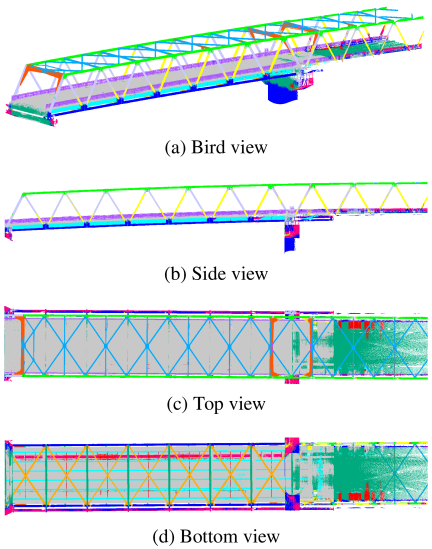
Fig. 22. The result of the segmentation members (colors are corresponded to the label in Fig. 12).
4.2. Segmentation Members from Point Cloud
3,476 training data and 5,000 validation data are created. Cross-sectional point clouds are detected at 0.02 m intervals from the starting point, and \(d\) is set as 0.01. Training took about 18 hours, and Intersection over Union (IoU) is shown in Table 9. Predicting labels of the members in all validation data took 9.5 hours. Fig. 22 shows the result of segmentation. For comparison, the results obtained using the past method 5 are also shown in Fig. 23.
These differences are the method used to generate the point cloud data acquired as training data. The past methods sampled points on the surface of 3D CAD models, while the proposed method uses point clouds obtained through laser measurement simulation with Helios\(\texttt{++}\). All other parameters are unified. In the past methods, the slabs in panels 1, 6, and 7, which had poor laser measurement quality, had many points mistaken for the cross beams. On the other hand, the proposed method correctly identified the slab, confirming an improvement in segmentation accuracy. However, the classification accuracy for the brace H and the box decreased slightly.
Since points were sampled on the surface of the 3D CAD data in the past research, there were no missing or noise associated with laser measurement, and points were generated even for internal areas not hit by the laser. Therefore, members containing missing area were segmented in low accuracy. In this research, segmentation accuracy was improved by using Helios\(\texttt{++}\) to acquire poor-quality point clouds closer to real laser measurements as training data.
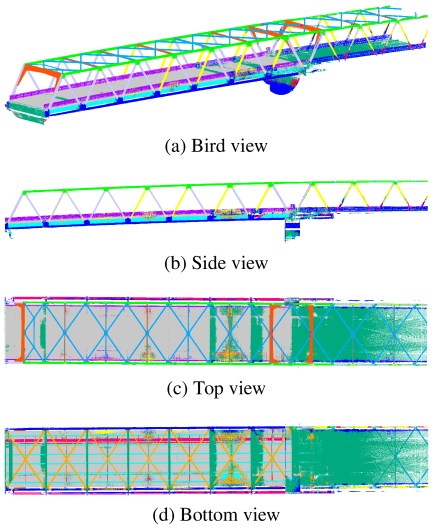
Fig. 23. The result of the past methods 5 (colors are corresponded to the label in Fig. 12).
However, this result may also be attributed to the fact that the measurement points in Helios\(\texttt{++}\) were identical to those in the actual measurements, leading to similar patterns of missing data and consequently reducing misclassification. When generating learning data, cases where the actual measurement locations are unknown are anticipated. Therefore, it is also necessary to develop techniques for setting measurement points where laser measurement is realistically feasible, such as beneath girders and sidewalks.
Furthermore, although the 3D CAD model in this research corresponds to the A1-P1 span and the laser measurement data correspond to the P4-A2 span, which has different structures, the bridge itself is the same, and therefore their shapes are similar. In the future, we aim to develop a model that integrates point cloud data from different truss and girder bridges with similar substructures below a slab.
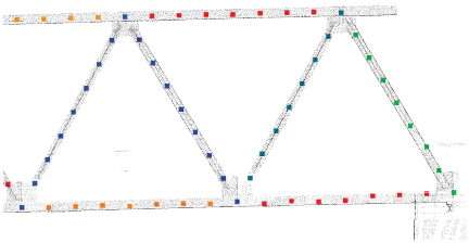
Fig. 24. Created center lines (panels 6 and 7, right side).
4.3. Creating Center Lines from Point Cloud Data
As shown in Fig. 24, the grid points are created in the center of the members. The sampled and adjusted points are generally centered, but on panel 7, which has many missing points, misalignment has occurred.
While the method for obtaining the center lines from the centroids of a cross-section can reproduce curvature, they are vulnerable to defects and noise. It is necessary to improve techniques capable of addressing these issues. Furthermore, a method for quantitatively evaluating the accuracy of center lines extracted from point cloud has not yet been established. It is necessary to explore evaluation methods, such as comparing them with the center line measurement methods used in practical bridge maintenance and management.
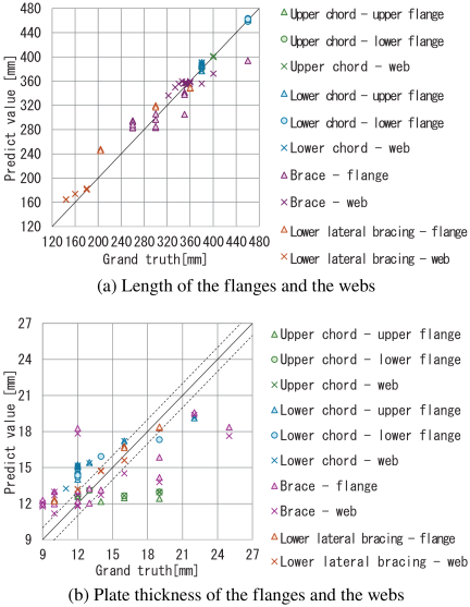
Fig. 25. Validation of predict cross-sectional geometries by using measured point clouds.
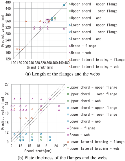
Fig. 26. Result of the past research 4.
4.4. Detecting Cross-Sectional Geometries from Point Cloud Data
The predicting result was the average of the predicted values obtained when inputting the cross-sectional point clouds of each single member. For comparison, results obtained using the author’s past method 4 are also shown. Here, only the lengths and thicknesses of flanges and webs were automatically extracted from point cloud data measured using the handheld laser scanner. As described in Section 2.2.2, the members that could be measured using the handheld laser scanner are limited. Therefore, the same value is applied here for the lower chords, braces, and lower lateral bracings as representative values for entire bridges. Since the upper chords were out of measurement reach, the results from the lower chord members with a similar shape were applied.
The result of the proposed method is shown in Fig. 25 and one of the past methods is shown in Fig. 26. The predicted plate thickness of the upper chords is smaller, while the predicted plate thickness of the lower chords is larger. The members with large errors in the braces were those containing gate frames and those with greater length or plate thickness compared to others.
The upper chord and lower chord only differ in plate thickness, and the measurement quality from the laser scanner is poor. On the other hand, the lower lateral bracings, which have relatively high predict accuracy, exhibit a certain degree of proportionality between length and plate thickness. From this, it can be considered that members where only the plate thickness has changed are difficult to predict. When validated with training data, the accuracy is high. But as shown in Fig. 27, the point cloud data acquired by the laser scanner and Helios\(\texttt{++}\) seem to be similar. One possible reason is that the noise and missing data patterns in Helios\(\texttt{++}\) vary slightly from panel to panel, and the model may have learned to adapt to those specific patterns. This indicates that there is potential to enhance robustness not only through the geometric characteristics of the cross-section but also by considering which panel it is (i.e., how far it is proportionally from fixed or movable supports).
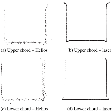
Fig. 27. Examples of cross-sectional point clouds.
Furthermore, challenges remain regarding normalization methods. Some cross-sectional point clouds sliced along the longitudinal direction are not perpendicular to the members. Therefore, when using point cloud from multiple bridges as training data, a projection onto a perpendicular cross-section is required. To achieve this, a centroid of the cross-section must be identified, and the direction vector of a center line must be determined. However, as discussed in Section 4.3, these processes are sensitive to noise and missing data. Consequently, methods robust to such uncertainties need to be developed in conjunction with center line detection.
5. Conclusion and Future Works
In this research, the improved methods of the three main steps (“segmentation members,” “creating center lines,” and “detecting cross-sectional geometries”) are proposed to construct fiber-based models semi-automatically from point cloud data of steel truss bridges.
Acquiring training data using Helios\(\texttt{++}\) enabled to obtain data closer to point cloud data acquired by more realistic laser scanners, thereby improving segmentation accuracy and cross-sectional geometries prediction accuracy in areas with missing data. However, since the training data were generated from the 3D CAD models of the same bridge with different spans, it was identified that the following improvements are necessary: adding training data generated from the 3D CAD models of different truss bridges, enhancing robustness against missing data and noise in center line detection, and investigating appropriate measurement conditions for Helios\(\texttt{++}\).
Furthermore, since the prediction accuracy for members like upper chords and lower chords, where only the plate thickness varies, was low, we aim to narrow the threshold and improve accuracy by utilizing the span length, panel length, width, and position relative to the support points of the truss bridge, rather than blindly learning only the shape. In addition, we will continue to work on improving methods for detecting a center line for quantitatively evaluating accuracy, and refining the normalization process when importing point clouds from other truss bridges and girder bridges.
Acknowledgments
This research was supported by the Foundation of Public Interest of Tatematsu (Nao Hidaka). The laser measurements were made with the help of Mr. Naofumi Hashimoto, Kameta Corp., Japan.
- [1] M. E. Mabsout, K. M. Tarhini, G. R. Frederick, and C. Tayar, “Finite-element analysis of steel girder highway bridges,” J. of Bridge Engineering, Vol.2, No.3, pp. 83-87, 1997. https://doi.org/10.1061/(ASCE)1084-0702(1997)2:3(83)
- [2] T. Nakamizo and M. Nishio, “Shell model reconstruction of thin-walled structures from point clouds for finite element modelling of existing steel bridges,” Sensors, Vol.25, No.13, Article No.4167, 2025. https://doi.org/10.3390/s25134167
- [3] K. Komuro, Y. Miyamori, M. Yoshida, T. Kadota, and T. Saito, “Construction of a point cloud FE model for a real structure with local damage and evaluation of its element shape,” Proc. of IABSE Symp. 2025, pp. 2925-2933, 2025. https://doi.org/10.2749/tokyo.2025.2925
- [4] N. Hidaka, N. Hashimoto, T. Nonaka, M. Obata, K. Magoshi, and E. Watanabe, “Construction of a practical finite element model from point cloud data for an existing steel truss bridge,” Proc. of the 23th Int. Conf. on Construction Applications of Virtual Reality (CONVR 2023), pp. 1155-1166, 2023. https://doi.org/10.36253/979-12-215-0289-3.114
- [5] N. Hidaka, N. Hashimoto, E. Watanabe, and D. Uchiyama, “Developing a deep learning-based method to segment bridge members by using 2D cross sectional point clouds,” Proc. of 13th Int. Conf. on Structural Health Monitoring of Intelligent Infrastructure (SHMII-13), pp. 550-557, 2025. https://doi.org/10.3217/978-3-99161-057-1-083
- [6] L. Winiwarter, A. M. Esmorís Pena, M. Yermo García, J. Martínez Sánche, M. Searle, H. Weiser, K. Anders, B. Höfle, and D. Kempf, “HELIOS++ (v2.1.0),” Zenodo, 2025. https://doi.org/10.5281/zenodo.16780208
- [7] N. Hidaka, T. Michikawa, A. Motamedi, N. Yabuki, and T. Fukuda, “Polygonization of point cloud of tunnels using lofting operation,” Int. J. Automation Technol., Vol.12, No.3, pp. 356-368, 2018. https://doi.org/10.20965/ijat.2018.p0356
- [8] M. A. Fischler and R. C. Bolles, “Random sample consensus: A paradigm for model fitting with applications to image analysis and automated cartography,” Communications of the ACM, Vol.24, No.6, pp. 381-395, 1981. https://doi.org/10.1145/358669.35869
- [9] D. H. Ballard, and C. M. Brown, “Region growing,” Computer Vision, Prentice Hall, pp. 149-165, 1982.
- [10] C. R. Qi, L. Yi, H. Su, and L. J. Guibas, “PointNet++: Deep hierarchical feature learning on point sets in a metric space,” Proc. of the 31st Int. Conf. on Neural Information Processing Systems, pp. 5105-5114, 2017.
- [11] R. B. Rusu and S. Cousins, “3D is here: Point cloud library (PCL),” 2011 IEEE Int. Conf. on Robotics and Automation (ICRA), 2011. https://doi.org/10.1109/ICRA.2011.5980567
This article is published under a Creative Commons Attribution-NoDerivatives 4.0 Internationa License.