Research Paper:
Stochastic Multi-Objective Sales and Operations Planning with Plan Stability Objectives and Supply Order Allocation Using Simulation–Optimization
Yigedeb Abay†
 , Toshiya Kaihara
, and Daisuke Kokuryo
, Toshiya Kaihara
, and Daisuke Kokuryo
Graduate School of System Informatics, Kobe University
1-1 Rokkodai-cho, Nada-ku, Kobe, Hyogo 657-8501, Japan
†Corresponding author

Sales and operations planning (S&OP), despite its importance in balancing demand and supply, faces significant challenges due to system complexity, uncertainty, and conflicting objectives. While previous research has primarily examined the effects of integration, flexibility, and inventory control on cost and customer service level under demand uncertainty, it has often overlooked the simultaneous consideration of plan stability, procurement time uncertainty, and supplier capacity constraints. This study addresses these gaps by developing a multi-objective S&OP simulation–optimization model that jointly considers plan stability objectives and capacity-constrained supply order allocation under both demand and procurement time uncertainty. Computational results from an automotive industry case study show that frozen horizon length has a more significant impact on customer service, delivery time, and plan stability than on total profit. A bi-sourcing policy proved more advantageous than single sourcing even under unlimited capacity and lower unit costs, while moderate procurement lead-time uncertainty outperformed deterministic lead times under long supply intervals. This reveals counterintuitive temporal supply dynamics in which lead-time overlaps and order crossings yield favorable logistics cost trade-offs. The results also indicate that sourcing policies, supply intervals and lead-time uncertainty influence plan stability even when frozen horizon length is fixed. These findings provide manufacturers with insights to balance flexibility and stability in S&OP, while managing multiple uncertainty sources and multi-sourcing strategies in dynamic supply chain environments.
S&OP simulation-optimization framework
1. Introduction
Sales and operations planning (S&OP), a core component of supply chain planning, plays a critical role at the tactical planning level by balancing demand and supply in today’s competitive manufacturing environment. It enables cross-functional integration and supports the achievement of a firm’s strategic objectives by aligning tactical decisions with the master production schedule (MPS). However, S&OP faces major challenges due to its large scale, complex nature, and the presence of uncertain parameters and multiple objectives. These challenges require broader integration, modeling of multiple uncertainty sources, development of efficient solution methods, and contextualization of existing models in different industrial environments 1. The broader production planning and supply chain management literature also emphasizes the importance of tactical decisions such as flexible capacity utilization, safety stock management, handling plan instability, and appropriate sourcing and order allocation policies in managing uncertainty 2,3.
Previous studies have primarily examined the effects of S&OP, integration level, and rolling planning horizons on system performance 4,5 as well as the design of manufacturing flexibility and inventory control policies using simulation–optimization approaches 6,7,8. In our previous work 9, we adapted an S&OP simulation model from the literature 6 to enhance its practical relevance in the context of the Ethiopian automotive industry. That study extended the cost objective to include total profit and price revision and introduced negotiated backup supply to minimize sales loss. While these studies focus on cost, profit, and customer service under demand uncertainty, simultaneous consideration of plan stability, procurement time uncertainty, and capacity-constrained supply order allocation at the S&OP level remains unexplored. Addressing this gap is relevant as manufacturers in global supply chains face high uncertainty and long-distance sourcing, leading to frequent plan changes, higher costs, longer delivery times, and lower customer service.
Plan instability or nervousness is associated with excessive schedule changes, which can reduce productivity, lower employee morale, and increase costs 10. This is typically addressed by freezing a portion of the plan that fixes production quantities for those periods in advance. This portion, known as the frozen horizon, stabilizes the production plan because new customer orders can only be placed afterward. Adjusting its length can be beneficial as managers frequently face trade-offs between maintaining stability and adapting to changing market and supply conditions, including flexible delivery time requirements 6,10. While a few previous studies explicitly consider plan stability in S&OP 11,12, they focus on MPS disaggregation under demand uncertainty using mathematical programming. This highlights a research gap regarding the interaction between supply-side factors and plan stability at the S&OP level.
The objective of this study is to develop and evaluate an integrated S&OP simulation–optimization model that incorporates capacity-constrained supply allocation under demand and procurement time uncertainty while explicitly considering plan stability objectives. The simulation model from our previous study 9 is extended into a simulation–optimization framework. The model is evaluated under varying frozen horizon lengths and supply-side factors, including sourcing policies, supply intervals, and lead-time uncertainty using a real-world automotive industry case. The originality of the study lies in incorporating key performance indicators (KPIs) of delivery time, plan instability, and nervousness alongside total profit and customer service, enabling informed decisions on frozen horizon adjustments and delivery time flexibility; integrating capacity-constrained supply allocation under multiple uncertainty sources by introducing order allocation percentage decision variables in addition to flexibility degree and safety stock ratio; and simultaneously evaluating S&OP performance and plan stability under varying frozen horizon lengths and supply-side factors.
The study’s contribution is an integrated S&OP model that incorporates plan stability objectives and capacity-constrained supply allocation, providing a comprehensive decision-making framework to balance plan stability and flexibility. The model extends the S&OP literature by addressing diverse objectives in long-distance and highly uncertain sourcing contexts prone to lead-time overlaps and order crossings. It further reveals counterintuitive insights arising from overlapping procurement times in multi-sourcing policies and from interactions between supply intervals and lead-time uncertainty. The model provides manufacturers with insights into how supply-side factors affect plan stability and supports managing the complexity of S&OP arising from multi-sourcing, multiple uncertainty sources, and supplier capacity constraints.
The remainder of the paper is structured as follows. Section 2 reviews the literature, Section 3 defines the problem and presents the model, and Section 4 outlines the simulation–optimization process and experimental design. Section 5 reports the results, Section 6 discusses the findings and their implications, and Section 7 concludes with suggestions for future research.
2. Literature Review
Demand-driven S&OP aims to synchronize production with uncertain demand in increasingly integrated, flexible, and globalized supply networks. This task is further complicated by uncertainties in both demand and procurement lead times 13,14. Managing such complexity and uncertainty and the associated risks requires flexible and responsive planning, real-time data integration, and the application of IT technologies and scenario planning within S&OP 15,16. Multiple sources of uncertainty reduce analytical tractability, necessitating computationally efficient approaches, such as simulation and AI-based methods 17. Simulation–optimization grounds models in practice and captures dynamic system behavior, but its effectiveness depends on data availability and quality, and interpreting and communicating results to decision makers remains challenging 18,19,20.
Prior studies consistently showed that a higher freeze proportion reduced instability but increased cost and reduced customer service 21,22,23. In capacitated systems under uncertain demand, shorter freeze lengths led to higher costs and lower service levels due to frequent replanning, whereas a longer total planning horizon improved capacity utilization and customer service but increased total cost and schedule instability 23,24. Nevertheless, reduced plan instability could be achieved with minimal cost increases, suggesting that longer freeze intervals and frequent replanning may be cost-effective 25,26. The use of end-item safety stock alongside freezing improved plan stability, fill rate, and total cost 27. These MPS-focused studies emphasized that frozen horizon length selection should balance trade-offs among cost, customer service, and plan stability, providing a theoretical foundation for supply-chain-level research on plan flexibility and stability.
Empirical studies have highlighted that relationships among supply chain members affect plan instability, and higher firm performance requires supply-chain-level flexibility, a factor often underestimated by manufacturers 28,29. Schedule stability can be achieved through component commonality, lower product variability, and coordination strategies such as S&OP. Mitigating the cost of instability requires longer frozen periods, whereas excessive flexibility increases instability, making the trade-off between these objectives a key focus of research 30. A hierarchical disaggregation planning study demonstrated the importance of a stable and high-quality S&OP for achieving a stable and optimal MPS 12. Incorporating a plan stability objective into aggregate production planning with dynamic flexibility bounds outperformed traditional single-cost-objective models in addressing nervousness as well as demand trends, seasonality, and uncertainty 31. These studies examined plan stability under production capacity constraints and demand uncertainty without fully addressing supply-side factors such as sourcing policies, supply intervals, and lead-time uncertainty.
Order allocation decisions to balance uncertain demand with supplier capacity require not only optimization but also simulation-based methods 32. While multi-sourcing can enhance customer service and reduce safety stocks and shortage costs, selecting suppliers with varying costs and allocating orders under budget and service level constraints remain challenging 3. Previous studies highlighted gaps in addressing multiple sources of uncertainty, developing simplified replenishment and order allocation policies, and applying simulation–optimization approaches 3,32,33. Moreover, real-world problems are inherently multi-objective with solution complexity arising from integer, nonlinear, and stochastic parameters 34. Hybrid algorithms in most commercial computer applications have improved the effectiveness of simulation–optimization techniques for solving complex problems such as supplier selection and order allocation 35.
More recent studies on S&OP showed that a linear policy that adjusts flexibility degree and safety stock ratio in each planning cycle outperformed static policies, even when backup supply unit costs were higher and uncertain 7,8. A contextualized S&OP model introduced negotiated backup supply and demonstrated improvements in total profit and customer service 9. In these studies, the frozen horizon was treated as a fixed parameter reflecting industry practice, in which it is predetermined for specific product models; however, adjusting it may help balance plan stability and delivery time flexibility 6. Such adjustment is crucial for adapting to evolving market and supply conditions, which necessitates the incorporation of plan stability and delivery time objectives. Moreover, these studies assumed deterministic procurement times and unlimited supply capacity without fully accounting for the operational constraints in global supply chains.
Overall, S&OP studies have largely addressed plan stability and supply allocation in isolation, often under production capacity constraints, and demand uncertainty assuming fixed frozen horizons, deterministic procurement times, and unconstrained supply capacity. Limited attention has been given to addressing multiple sources of uncertainty and examining the effects of supply-side factors on plan stability. To address these gaps, this study develops an S&OP simulation–optimization model that incorporates plan stability objectives and integrates capacity-constrained supply allocation under both demand and procurement time uncertainty. The S&OP model is examined under varying frozen horizon lengths, sourcing policies, supply intervals, and procurement time uncertainty levels.
Source: 9
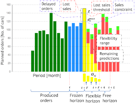
Fig. 1. Order placement against predicted demand. The box on the first yellow bar marks the time fence, where orders are subject to a sales constraint check. Dark green bars represent previously produced orders, with blue and yellow bars indicating the current planning horizon.
3. Problem Definition and Formulation
This section defines and formulates the integrated S&OP problem addressed in this study. The problem involves placing stochastic demand within a rolling planning horizon, where a frozen horizon with a time fence stabilizes production schedules and a flexible horizon allows future adjustments (Fig. 1). The model captures the effects of frozen horizon length on delivery time, customer impatience, and service level. It also accounts for uncertain procurement times from multiple long-distance suppliers, which can lead to overlapping lead times and order crossings between planning cycles. Supply requirements are split among capacity-constrained suppliers and placed under uncertain lead times, potentially causing shortages or excess inventory. Incorporating plan instability and local and global nervousness objectives allows informed decisions regarding frozen horizon length adjustments and delivery time flexibility. The S&OP simulation–optimization framework determines the flexibility degree, safety stock ratio, and supply allocations to maximize total profit while satisfying constraints on delayed orders, lost sales, delivery time, plan instability, and nervousness.
The first subsection outlines the customer order placement, flexibility, and inventory control components of the S&OP model, which provides the baseline for the proposed extensions. The subsequent subsections include the effects of frozen horizon adjustments, incorporation of plan stability objectives, modeling of procurement time uncertainty, integrating capacity-constrained supply order allocation, and optimization of the integrated S&OP system. Table 1 lists the notations for the planning, demand and sales, supplier, cost, and capacity parameters used as simulation inputs. The demand and inventory variables are determined through simulation and used to compute the KPIs. The table also lists the optimization decision variables.
Table 1. S&OP system parameters, variables, and KPIs.

3.1. Baseline S&OP Model: Order Placement, Flexibility, and Inventory Control
The baseline model considers highly unpredictable customer demand with no significant trend or seasonality. In such cases, customer demand arrival is modeled as a uniformly distributed random parameter. High forecasting errors, which are common with long procurement times that can lead to unreliable demand predictions, are also incorporated in the model 2,6. Predicted demand is calculated as the sum of the actual demand arrival and a uniformly distributed forecasting error, as shown in Eq. \(\eqref{eq:1}\).
As illustrated in Fig. 1, the rolling planning horizon comprises a frozen horizon (\(t\) to \(t+F-1\)), a flexible horizon (\(t+F\) to \(t+F+4\)), and a free horizon beginning at \(t+F+5\). The actual demand arrival (\(D_t^a\)) at period \(t\) is allocated to future periods \(j\) within the flexible horizon in fractional quantities (\(O_{tj}\)), as defined in Eqs. \(\eqref{eq:2}\) and \(\eqref{eq:3}\). These fractions are aggregated at each replanning cycle and become actual orders \(d_t^a\) (yellow bars in Fig. 1). Order-placing factors (\(x_{j-t}\)) represent the demand arrival rates estimated based on industrial data 6. These customer orders are placed independently of the predicted demand (red) and parts availability. The order placement factors used in this study are listed in Table 2.
Table 2. Order-placing factors. Source: 8.

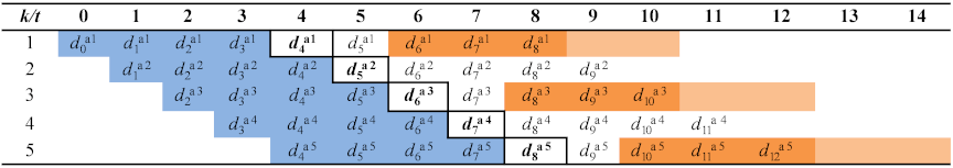
Fig. 2. Sample plan illustrating actual orders placed within the frozen and flexible horizons and supply arrival times.
At the time fence (\(t+F\)), the maximum number of orders that the sales department can accept subject to manufacturing capacity limits are defined by the sales constraint (\(d_t^{\textit{max}}\)), as illustrated in Fig. 1. This constraint, which includes an allowance above the predicted demand, is calculated using the flexibility degree in Eq. \(\eqref{eq:4}\) 6. It defines the flexibility range (light green) beyond which customer orders are delayed or lost. Delayed orders are backorders caused by capacity limits, i.e., the sales constraint at a future time fence period, and should not be confused with execution-level delivery delays in the current period, which are mitigated through backup supply. As the planning horizon rolls forward, the remaining actual orders to be produced, i.e., the production order quantity (\(N_t=\min\{d _t^a;d_t^{\textit{max}}\}\)), enter the frozen horizon, where no further changes are allowed. Under this strict time-based rule, no new orders are placed into frozen periods, even if the production quantities are below the available capacity. Any remaining predicted demand (\(d_t^{\textit{pr}}=\max\{0;d_t^p-d_t^a\}\)) is removed from the frozen horizon.
The flexibility degree determines the sales constraint, whereas the safety stock ratio functions as a supply buffer that accounts for customer order variability within the flexible horizon. In practice, these variables are determined through negotiation among the sales, manufacturing, and logistics departments and remain fixed throughout each planning cycle. In contrast, the linear policy defined in Eqs. \(\eqref{eq:5}\) and \(\eqref{eq:6}\) enables dynamic adjustment of both variables at each planning cycle and has been demonstrated to outperform the static policy 7. The decision variables are the absolute and relative coefficients of flexibility degree \((\textit{FR}^{\alpha },\textit{FR}^{\beta})\) and the safety stock ratio \((\textit{SS}^{\alpha},\textit{SS}^{\beta})\). The parameter \(\varPhi_t\) in Eq. \(\eqref{eq:7}\) represents the ratio of the expected demand to the historical moving average of the predicted demand over \(M\) periods. When expected demand exceeds the moving average (\(\varPhi_t>1\)), demand is overestimated, resulting in a lower flexibility degree and a lower safety stock ratio to avoid unused capacity and excess inventory. Conversely, when \(\varPhi_t<1\), demand is underestimated, leading to higher flexibility and safety stock to prevent delayed orders and stockouts.
3.2. Effects of Frozen Horizon Length Adjustments
The frozen horizon length determines the time fence position and fixes orders within those periods, thereby stabilizing manufacturing and logistics operations. Fig. 2 illustrates a sample plan with actual orders (\(d_t^{ak})\) for planning cycle \(k\) and period \(t\). Blue-shaded periods denote the frozen horizon, while the remaining periods represent the flexible horizon. The time fence periods are marked in bold within boxes. Together, these sections constitute the total planning horizon (PH), which rolls forward by one period at each planning cycle. Orange-shaded periods are supply arrival times, which are discussed in the next subsection.
In the automotive industry, especially where imported vehicles often outcompete locally manufactured models, customer impatience is higher. Longer frozen horizons lead to extended delivery times, thereby increasing the risk of lost sales, whereas shorter horizons enhance responsiveness and increase tolerance for backorders. Delayed orders and lost sales are determined by the sales constraint and lost sales threshold (\(Z\)) (Fig. 1). The threshold represents customer impatience beyond which customers cancel their orders 8. In this study, the lost sales threshold is modeled relative to the frozen horizon length to capture the effects of customer impatience in S&OP. This relationship is estimated based on the customer impatience level toward backordering in the case industry and is used in the simulation model (Table 3). Actual orders exceeding the sales constraint, but within the threshold are delayed to the next period, as in Eq. \(\eqref{eq:8}\), whereas any excess orders beyond the threshold are lost, as in Eq. \(\eqref{eq:9}\).
The effects of frozen horizon adjustments on delivery time flexibility and plan stability necessitate the introduction of both objectives within the S&OP model. The formulation for the average delivery time is presented below, and incorporation of plan stability objectives is discussed in the subsequent subsection.
Table 3. Relationship between frozen horizon length and lost sales threshold.

The model measures the average promised delivery time assigned to outstanding orders within the current planning horizon, considering frozen and flexible horizon lengths, delayed orders, and lost sales. As shown in Eq. \(\eqref{eq:10}\), it is calculated as the weighted average of the actual orders from the upcoming period (\(t+1\)) to the end of the planning horizon (\(t+F+4\)), where each order is weighted by its respective period \(m\), divided by the total number of actual orders. This represents the average due date of all orders in the current planning horizon waiting to be fulfilled averaged over the simulation length \(H\).
3.3. Incorporating Plan Stability Objectives
To evaluate schedule changes within the rolling-horizon planning framework, explicit KPIs for plan instability and local and global nervousness are incorporated in the S&OP model. Schedule changes emerge from frozen horizon length adjustments, sales constraints imposed on actual demand at the time fence, and the aggregation of customer orders within the flexible horizon. Using the sample plan shown in Fig. 2 (Section 3.2), these KPIs are defined and introduced in the model as follows.
Capturing intra-cycle actual order variability between periods is crucial because it quantifies how fluctuations in production quantities affect capacity utilization, production flow, and supply order consistency within the rolling planning horizon. Plan instability therefore measures the average difference (smoothness) in scheduled quantities between consecutive periods within the same planning cycle 12,22. As shown in Fig. 2 and Eq. \(\eqref{eq:11}\), for Planning Cycle 5 at Period 4, it is computed as the sum of absolute differences in actual orders between two consecutive periods from Period 4 to Period 11 divided by the total number of periods minus one.
A plan may be internally smooth within a cycle yet undergo frequent adjustments across cycles, increasing the coordination burden across functions, reducing productivity and worker morale, and causing supplier dissatisfaction. Plan nervousness measures changes in order timing or quantity in the current or lower-level schedules due to minor adjustments at higher or similar planning levels 12,22. Local nervousness for Planning Cycle 5 at Period 4 is computed as the sum of the absolute changes that the actual order quantity (\(d_4^{a5}\)) has undergone from Planning Cycles 1 to 5 in Period 4, divided by its current value (Eq. \(\eqref{eq:12}\)). Global nervousness extends this calculation across the entire planning horizon by summing the absolute changes the actual orders have undergone from Planning Cycles 1 to 5 for each period from \(t=4\) to \(t=11\), divided by the total of actual orders in the current cycle (Eq. \(\eqref{eq:13}\)). These KPIs are averaged over the simulation length.
3.4. Modeling Procurement Time Uncertainty
Procurement time in global supply chains is typically long and highly uncertain. Lead times for different orders can become independent of each other, making the modeling difficult because the arrival times can cross despite the sequence in which they were placed. Most studies in the literature did not allow order crossing, assuming that the interval between orders is usually large enough 36. In this study, we consider a short normal supply interval (NSI) and allow the possibility of order crossing due to higher uncertainty in distant sourcing. Moreover, multi-sourcing introduces additional variations in supplier lead times. Thus, orders placed in a certain period may arrive either earlier or later than the expected arrival time (\(t+L\)), leading to concurrent or missed arrivals and resulting in excess inventory or shortages.
The supplier lead times (\(L_{it}\)) are modeled as uniform distributions (Fig. 2). The figure shows the supply orders from two suppliers placed at \(k=1,3,5,\dots\) (\(\textit{NSI}=2\)). It shows overlapping (orange-shaded) and non-overlapping (light orange) supply arrivals as well as order crossings between cycles. The expected arrival lead time \(L\) is determined by averaging the minimum and maximum lead times of each supplier (\(L_i^{\textit{min}}\) and \(L_i^{\textit{max}}\)) within their respective distributions, as shown in Eq. \(\eqref{eq:14}\). This value is used to determine the anticipated inventory and normal supply required in the next subsection.
3.5. Integration of Capacity-Constrained Supply Order Allocation
The case company procures vehicle parts as completely knocked down (CKD) units based on the demand plan. In the baseline S&OP model, the normal supply at \(t+L\) (Eq. \(\eqref{eq:16}\)) is calculated from the expected demand, the anticipated inventory at \(t+L-1\) (Eq. \(\eqref{eq:15}\)), and the safety stock ratio (determined in Section 3.1). The safety stock ratio provides a buffer for the expected changes in actual orders from period \(t+F+1\) to \(t+L\) 6.
However, the model assumes that the exact normal supply quantity arrives within a deterministic lead time and without capacity constraints. In practice, parts may be sourced from multiple suppliers with uncertain lead times and limited capacities. This study extends the model by computing the anticipated inventory and normal supply for the expected arrival period \(t+L\) (determined using Eq. \(\eqref{eq:14}\)) and splitting the normal supply required among suppliers using the newly introduced order allocation percentage decision variables (\(q_i\)), subject to capacity constraints and lead-time uncertainty.
The capacity of each supplier is modeled with minimum and maximum values based on its standard order quantity for initiating purchases and maximum production capacity. Accordingly, the allocated orders for each supplier subject to their respective capacity limits are determined as shown in Eq. \(\eqref{eq:17}\). Because each supplier has an uncertain lead time, deviations can occur between the required normal supply at \(t+L\) and the realized supply due to different arrival times (\(t+L_{it}\)). This can result in missed or concurrent arrivals, causing shortages or excess inventory that reflect the degree of lead-time overlap within the same planning cycle (Fig. 2). Similarly, lead-time overlap between planning cycles, i.e., order crossing, can occur depending on the normal supply interval.
The realized normal supply at period \(t\) is compiled as in Eq. \(\eqref{eq:18}\) considering the concurrently arriving orders placed at \(t-L_{it}\) from different suppliers and planning cycles. The parameter \(c\) is used to determine the range of possible previous planning cycles (\(k\)) at which separate orders may cross and arrive concurrently. It is calculated as \(c=\max\{L_i^{\textit{max}}\}-\min \{L_i^{\textit{min}}\}\). If \(\textit{NSI}>c\), order crossing does not occur. The simulation model compiles the total realized normal supply (\(n_t^R\)) from each supplier’s normal supply arrival (\(n_{it}\)) ordered over the range of \(k\) cycles as defined in the equation.
Backup supplies are modeled following previous studies. When a shortage occurs in period \(t\), a primary backup supply is ordered and arrives within the same period, as in Eq. \(\eqref{eq:19}\) 6. In addition, a negotiated backup, as in Eq. \(\eqref{eq:20}\), is used to improve customer service and total profit. This supply is scheduled for period \(t+F\) after negotiation with impatient customers who might otherwise cancel their orders, and is estimated from sales at risk of being lost and the probability of customer agreement 9. Both backup supply types are not subject to supply capacity constraints and incur higher unit costs than normal supply. The resulting net actual inventory at the end of period \(t\) is determined using Eq. \(\eqref{eq:21}\).
3.6. Optimization of the Integrated S&OP System
The model also incorporates conventional KPIs, such as total profit and the percentages of delayed orders and lost sales. They are introduced prior to formulating the integrated S&OP optimization model. The price factor in Eq. \(\eqref{eq:22}\) is included in the profit calculation to compensate for the negotiated backup supply costs covered by customers who accepted the negotiated delivery, thereby avoiding backorders. Manufacturing cost considers overtime when the production order quantity (\(N_t\)) exceeds the normal manufacturing capacity (\(N\)), as in Eq. \(\eqref{eq:23}\). Based on the previously determined variables and unit cost data, the average total profit over the simulation length is calculated using Eq. \(\eqref{eq:24}\) 9. Customer service performance is measured through delayed-order and lost-sales percentages, defined as the ratio of delayed orders and lost sales to the total actual orders across the simulation length, as shown in Eqs. \(\eqref{eq:25}\) and \(\eqref{eq:26}\) 6.
The integrated S&OP model considers total profit, delayed-order and lost-sales percentages, average delivery time, plan instability, and nervousness as inherently conflicting objectives that require multi-objective optimization. Decision variables include the absolute and relative coefficients of flexibility degree and safety stock ratio, and order allocation percentages. Increasing flexibility improves service levels but may lead to excessive backup supply costs and lower profits. Higher safety stocks reduce shortages but increase inventory holding risks under demand and lead-time uncertainty. Longer frozen horizons enhance schedule stability but may extend delivery times, raise costs, and increase lost sales, reflecting the inherent trade-offs among the objectives.
To manage these trade-offs, the \(\varepsilon\)-constraint method is applied, scalarizing the optimization problem into a single objective with one primary objective and the others as bounding constraints. This approach ensures global optimality of the primary objective while maintaining Pareto optimality of the remaining objectives whose values typically lie near their respective \(\varepsilon\)-constraint bounds. This method is used because it effectively handles multiple conflicting objectives, allows decision makers to specify or validate acceptable bounds for secondary objectives, and enables efficient exploration of Pareto-efficient solutions.
Maximization of total profit is treated as the primary objective, while the \(\varepsilon\)-constraint objectives include maximum delayed-order and lost-sales percentages, delivery time, plan instability, and local and global nervousness denoted as DOP\(^{\textit{max}}\), LSP\(^{\textit{max}}\), \(T^{\textit{max}}\), \(I^{\textit{max}}\), LN\(^{\textit{max}}\), and GN\(^{\textit{max}}\), respectively. These values can be tuned to generate multiple viable solutions; however, careful consideration is required when dealing with a large number of objectives, as in this study 37. Accordingly, the \(\varepsilon\)-vector values were determined through iterative simulation experiments and subsequently validated by company experts. This process ensured feasible solutions and balanced trade-offs across conflicting objectives in the absence of predetermined company thresholds. The selected values are presented in Section 4.3.
The optimization model is formulated using Eqs. \(\eqref{eq:27}\)–\(\eqref{eq:35}\). Eq. \(\eqref{eq:27}\) defines the primary objective function, while Eqs. \(\eqref{eq:28}\)–\(\eqref{eq:33}\) specify the \(\varepsilon\)-constraints. Eq. \(\eqref{eq:34}\) represents the sum of the normal supply allocation percentages of suppliers, and Eq. \(\eqref{eq:35}\) imposes a nonnegative constraint on all decision variables.
4. Simulation–Optimization Process and Experimental Design
Simulation captures the arrival and scheduling of the uncertain customer demand within rolling frozen and flexible horizons, enabling dynamic interactions between manufacturing flexibility, backordering, and lost sales. It determines supply requirements with safety margins and allocates orders among multiple suppliers while accounting for capacity limits and lead-time variability. This provides a realistic system performance evaluation that would otherwise be difficult if analytical optimization were used independently. By separating system modeling from the solution procedure, simulation-based optimization enables algorithms in simulation software programs to solve such complex real-world S&OP problems efficiently 38.
4.1. Simulation Process
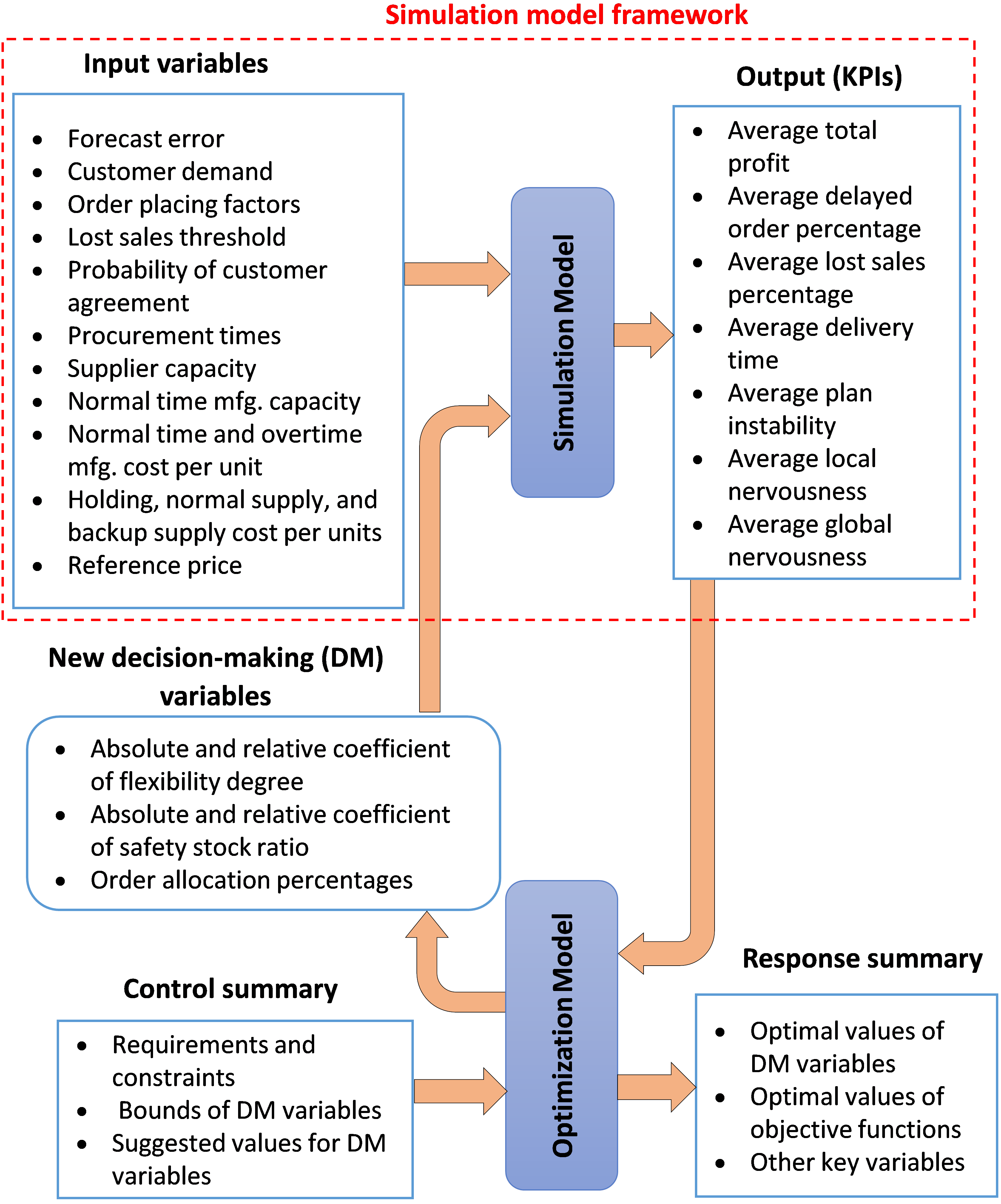
The model is developed using AnyLogic, a visual library-based simulation software with a three-phase and job-driven approach, enabling detailed and complex process modeling 39. The model inputs and outputs are shown in Fig. 3, and the simulation proceeds through the following major steps: (1) predicting demand for the entire simulation period, (2) determining expected procurement time, (3) handling demand arrival and customer order placement, (4) calculating flexibility degree and safety stock ratio, (5) determining delayed orders and lost sales, (6) calculating and placing negotiated backup supply, (7) evaluating average delivery time, plan instability, and nervousness KPIs, (8) calculating and placing primary backup supply, (9) determining actual and anticipated inventory levels and normal supply required, (10) splitting and placing supply orders based on allocation percentages considering capacity constraints and uncertain procurement times, (11) calculating total profit, and (12) determining the averages of KPIs and performance measures. Steps 2–11 repeat in each planning cycle as the planning horizon rolls forward by one period (month) throughout the simulation length. Step 12 is performed at the end of each simulation run of the optimization iterations.
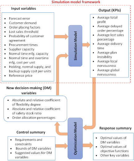
Source: Modified version from 8.
Fig. 3. Simulation–optimization process.
4.2. Optimization Process
Among the available optimization engines in AnyLogic, OptQuest is selected for this study because it combines scatter search, Tabu Search, and neural networks as primary search strategies, enabling it to efficiently handle the complex and multidimensional nature of the integrated S&OP problem and achieve faster convergence 40.
Figure 3 also shows the interaction between the simulation and optimization engines. The optimization engine first generates decision-making variables by considering their bounds, requirements, and suggested values. These variables, together with the input parameters, are entered into the simulation model to determine the KPIs. Each simulation run is repeated multiple times to account for demand and procurement time uncertainty. The optimization engine calculates the average of the KPIs from these replications and checks them against the \(\varepsilon\)-constraint limits. If any constraint is violated, the solution is deemed infeasible. Otherwise, the optimization engine compares the total profit from the current iteration with the previous best value. If a higher profit is found, it updates the best objective value and the corresponding solution. In the next iteration, the optimization engine searches for other decision-making variables in the solution space that can potentially maximize the total profit compared with the current best value. This iterative process continues until the maximum number of iterations is reached and an optimal solution is found. Whenever an iteration improves the primary objective, the decision variables, total profit, \(\varepsilon\)-constraint values, and key performance measures are recorded.
4.3. Industrial Case Study and Experimental Design
In our previous study 9, the Bishoftu Automotive Industry (BAI) case was used to contextualize and apply an S&OP model from the literature using simulation. In the present study, the case is updated with qualitative and quantitative data and used to evaluate the integrated S&OP simulation–optimization framework proposed. The updates include information on delivery time delays, rescheduling practices, customer behavior in response to backorders, key suppliers, and their attributes, including capacity, procurement lead-time and uncertainty, and unit supply costs.
BAI, an Ethiopian company, purchases automotive parts mainly from Chinese suppliers and sells assembled light pickup trucks, buses, and heavy-duty trucks in the local market. The double-cabin light pickup truck, which has a diverse customer base with small order quantities, is selected for this case study. The marketing and sales department prepares an annual demand plan with monthly breakdowns based on qualitative sales analysis and market research. The logistics department conducts international bids to select suppliers and procures parts once foreign currency exchange is secured. The procurement is carried out in CKD units, primarily from two major suppliers that have established long-term relationships with the company. The procurement lead times are long and uncertain with a uniform distribution. Customer orders are registered in advance while procurement of parts is underway.
The major challenges include high demand forecast errors, long and uncertain procurement lead times, and delayed deliveries. Extended procurement lead times result from international bidding processes and delays in securing foreign currency. Facing these supply constraints, the company adopts a risk-averse strategy of registering customer orders but postponing delivery commitments until parts physically arrive and repeatedly revising production plans based on the availability of parts. This often leads to low capacity utilization, delayed delivery times, and price fluctuations, which may lead to customer order cancelations.
The historical sales data show no significant trend or seasonality and follow a uniform distribution. The average customer demand is assumed to equal the full capacity of two 8-hr shifts per day throughout the month due to low capacity utilization. The collected company data include forecasting error, procurement lead times, normal supply cost per unit, inventory holding cost per unit per period, normal time manufacturing capacity, normal time manufacturing cost per unit, overtime-to-normal time manufacturing cost per unit ratio, and reference price. The relationship between the frozen horizon length and lost sales threshold, backup supply cost per unit, and supplier capacities are estimated for the study. The other input parameters are provided in Table 4. Due to confidentiality concerns, only some of the input parameters are presented in the table.
Table 4. Simulation–optimization input and control parameters.

Three experiments are designed and conducted to examine the effects of frozen horizon length adjustments and evaluate the impact of supply-side factors on system performance and plan stability objectives. The experiments further analyze the dynamic interactions among decision variables, internal (frozen horizon length, sourcing policy, and supply interval) and external (supplier capacity constraint, unit cost, and lead-time uncertainty) factors, and the trade-offs among objectives within the integrated model. The maximum values for the \(\varepsilon\)-constraints in all experiments are set as \(\textit{DOP}^{\textit{max}}=4.5\), \(\textit{LSP}^{\textit{max}}=2.5\), \(T^{\textit{max}}=4.25\), \(I^{\textit{max}}=25\), \(\textit{LN}^{\textit{max}}=0.980\), and \(\textit{GN}^{\textit{max}}=0.960\). The experiments and their corresponding descriptions are presented as follows:
Experiment 1: Effect of Frozen Horizon Length In this experiment, tests are conducted for frozen horizon lengths of 1–7 to evaluate their effects on system performance and plan stability. This also helps determine the appropriate length for use in subsequent experiments. The flexible horizon length is set to 5, causing the total planning horizon to increase with each frozen horizon increment. The absolute and relative flexibility degrees and safety stock ratios are the decision-making variables. Supplier 1, with a procurement lead time of \(L_{1t}=[6,10]\), is used without capacity restriction.
Experiment 2: Sourcing Policies In this experiment, the capacity constraints of Supplier 1 are applied, and Supplier 2 with a procurement time of \(L_{2t}=[6,8]\) is also utilized. However, the normal supply cost per unit of Supplier 2 is 1.5% higher than that of Supplier 1. The capacity of Supplier 1 is \({Ca}_1=[30,90]\), whereas that of Supplier 2 is unconstrained. Thus, four sourcing policies are designed and tested. Policy 1: Supplier 1 without capacity constraints; Policy 2: Supplier 1 under capacity constraints; Policy 3: Supplier 2 without capacity constraints; and Policy 4: bi-sourcing, where both Supplier 1 with capacity constraints and Supplier 2 without constraints are utilized. Here, the order allocation percentages (\(q_i\)) are considered as additional decision-making variables.
Experiment 3: Sensitivity to Normal Supply Interval and Procurement Time Uncertainty The sensitivity of the S&OP system is tested for three procurement time uncertainty levels under three NSI values. The procurement uncertainty levels are as follows. Deterministic: \(L_{1t}/L_{2t}=8/8\); Medium: \(L_{1t}/L_{2t}=[6,10]/[6, 8]\); and High: \(L_{1t}/L_{2t}=[4,12]/[4,10]\). Each uncertainty level is tested for NSI values of 1, 2, and 3. The S&OP system with the best-performing sourcing policy from Experiment 2 is used in this experiment.
5. Computational Results
This section presents the experimental results, including the decision variables, key performance measures, and optimal objective values. The key performance measures include the average flexibility degree (\(\textit{FR}_t\)), safety stock ratio (\(\textit{SS}_t\)), production order quantity (\(N_t\)), normal supply required (\(n_t\)), normal supply arrivals (\(n_{it}\)), primary backup supply (\(b_t^p\)), negotiated backup supply (\(b_t^n\)), actual inventory level (\(\textit{IL}_t\)), normal supply cost (NSC), backup supply cost (BSC), inventory holding cost (IHC), manufacturing cost (MC), and total sales (TS) calculated over the simulation length \(H\). The TS, NSC, BSC, IHC, and MC correspond to the components of total profit in Eq. \(\eqref{eq:24}\) and are listed in the same sequence. The coefficient of variation, standard deviation (\(s\)), and error bars are reported as needed, alongside the mean (\(\bar{x}\)) of the best iteration’s replications. Furthermore, a two-tailed paired \(t\)-test (\(\alpha=0.05\)) is conducted to determine whether the differences in optimal objective values and key performance measures between scenarios are statistically significant. Exact \(p\)-values are reported only when \(p \ge 0.001\), whereas results with \(p< 0.001\) are reported as statistically significant without exact values. The average computational time of each scenario in the experiments was 1 hour and 23 minutes.
5.1. Effect of Frozen Horizon Length
The results of Experiment 1 are summarized in Table 5 and Fig. 4. The table shows the freeze proportion for each frozen horizon length, defined as the percentage of frozen periods relative to the total planning horizon. The flexibility degree (\(\textit{FR}_t\)) decreased from its highest value at \(F=1\) to its lowest at \(F=6\), while the safety stock ratio (\(\textit{SS}_t\)) remained nearly zero, except at \(F=7\). As \(F\) increased from 1 to 7, the production order quantity (\(N_t\)) and normal supply arrivals (\(n_{1t}\)) decreased by 1.8% and 1.1%, respectively. Primary backup supply and actual inventory levels declined by 5.9% and 11.7%, respectively, whereas negotiated backup supply increased by 38.1%.
Table 5. Decision variables and key performance measures across different frozen horizon lengths.

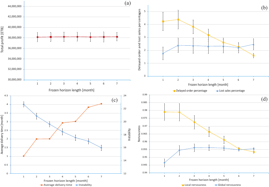
Fig. 4. Optimal objective values across different frozen horizon lengths.
Figure 4 shows the objective values, with the error bars representing the standard deviations. The error bars of the average delivery time are nearly invisible due to its very low variability. Overall, variability across replications was low, with a coefficient of variation below 10% for most objectives, indicating stable simulation performance. The lost sales exhibited a relatively higher coefficient of variation due to its small mean value.
Table 6. Performance of sourcing policies under different supplier constraints.

As shown in Fig. 4(a), the total profit in Ethiopian Birr (ETB) did not change significantly across all frozen horizon lengths (\(p=0.459\)), suggesting that it remains largely unaffected by freezing decisions. By contrast, delayed orders decreased substantially by 63.4% as \(F\) increased beyond 2, as shown in Fig. 4(b). Lost sales increased initially by 34.8% at \(F=2\) and remained stable through \(F=5\) before reaching its highest level at \(F=7\). This pattern suggests that excessive freezing shifts most unmet demand toward lost sales as customer impatience increases. Delivery time generally increased with longer frozen horizons, and only minimal increments were observed from \(F=2\) to 3 and \(F=3\) to 4 (Fig. 4(c)). Instability declined by 29.6% from \(F=1\) to 7. Local nervousness (Fig. 4(d)) similarly decreased by 2.6% beyond \(F=2\). In contrast, global nervousness increased by 1.0% from \(F=1\) to 3, remained stable through \(F=5\) (\(p=0.489\)), and then decreased slightly toward \(F=7\). These results indicate that delayed orders exhibited a pattern similar to local nervousness, while lost sales mirrored the trends of global nervousness.
Overall, longer frozen horizons reduced delayed orders, instability, and local nervousness without significantly affecting total profit. However, these improvements came at the expense of responsiveness, as reflected in higher lost sales, longer delivery times, and slightly elevated global nervousness. To balance stability and responsiveness, \(F=3\) was selected from the reasonable range (\(F=2\)–5) and used in the subsequent experiments.
5.2. Sourcing Policies
Table 6 presents the decision variables, key performance measures, and optimal objective values. Under Policy 2, the flexibility degree (\(\textit{FR}_t\)) decreased significantly, while the safety stock ratio (\(\textit{SS}_t\)) increased compared to Policy 1. The production order quantity (\(N_t\)) showed no significant change (\(p=0.371\)). The normal supply requirement (\(n_t\)) increased substantially, while arrivals (\(n_{1t}\)) declined due to capacity constraints. Consequently, backup supply cost increased, reducing total profit by 3.9% despite lower normal supply and inventory holding costs. Delayed orders and plan instability increased by 12.2% and by 2.1%, respectively. By contrast, lost sales, average delivery time, and local and global nervousness exhibited no significant changes (\(p=0.134\), 0.793, 0.271, and 0.338, respectively).
Under Policy 3, the flexibility degree declined relative to Policy 1, but less sharply than in Policy 2. The safety stock ratio, production order quantity, and both normal supply requirement and arrivals showed no significant changes. The normal supply cost increased, whereas the inventory holding cost decreased significantly. The backup supply cost, manufacturing cost, and total sales exhibited no significant changes (\(p=0.139\), 0.724, and 0.726, respectively). The decline in total profit (5.6%) was driven solely by the higher unit supply cost of Supplier 2, rather than by backup supply or inventory holding costs. Delayed order percentage and plan instability increased by 6.1% (\(p=0.016\)) and 0.8% (\(p=0.014\)), respectively. The lost sales percentage, average delivery time, and both local and global nervousness remained unchanged (\(p=0.771\), 0.338, 0.113, and 0.091, respectively).
Table 7. Sensitivity of S&OP performance to procurement time uncertainty under different normal supply intervals.

The bi-sourcing policy (Policy 4) showed the lowest flexibility degree and minimal safety stock ratio among all policies. Normal supply was allocated 68% to Supplier 1 and 32% to Supplier 2, with arrivals of 44.3 (33.7% of \(n_t\)) from Supplier 1 and 42.1 (32.0% of \(n_t\)) from Supplier 2, indicating that \(q_2\) was fully realized, whereas \(q_1\) was only partially fulfilled. The production quantity remained unchanged across all policies.
Compared to Policies 2 and 3, the bi-sourcing policy increased total profit by 4.8% and 6.7%, respectively. Delayed orders were unchanged relative to Policy 2 (\(p=0.302\)) but increased by 8.0% compared to Policy 3. Lost sales decreased significantly by 8.8% (\(p=0.006\)) and 5.3% (\(p=0.050\), actual value \(=0.0498\)), while delivery time shortened slightly by 0.05% compared to both policies (\(p=0.014\) and 0.002). Plan instability increased by 1.0% (\(p=0.009\)) and 2.3%, whereas both local and global nervousness declined by 0.3% and 0.2% relative to both policies. Compared to Policy 1, Policy 4 also improved total profit by 0.7% (\(p=0.015\)), shortened delivery time by 0.05% (\(p=0.022\)), and reduced local (\(-\)0.4%) and global (\(-\)0.2%) nervousness. Lost sales remained unchanged (\(p=0.163\)), while delayed orders and instability increased by 14.5% and 3.1%, respectively.
5.3. Sensitivity to Normal Supply Interval and Procurement Time Uncertainty
Table 7 presents the sensitivity analysis of procurement time uncertainty levels under different normal supply intervals (NSIs) using the bi-sourcing policy from Experiment 2. For improved readability, the cost and profit data in the table are reported in thousands. At \(\textit{NSI}=1\) and 3, the flexibility degree increased with greater uncertainty, while the safety stock ratio declined, indicating a shift to more responsive planning. At \(\textit{NSI}=2\), however, the highest flexibility degree and lowest safety stock ratio occurred at the medium uncertainty level, suggesting a nonlinear response to uncertainty. The production order quantity showed limited sensitivity overall, declining only at specific NSI–uncertainty combinations, such as at \(\textit{NSI}=1\) under medium (\(p=0.004\)) and high uncertainty, and at \(\textit{NSI}=3\) under medium uncertainty (\(p=0.010\)). Supplier allocation shifted with longer supply intervals, with \(q_1\) near 100% at \(\textit{NSI}=1\) and increased \(q_2\) shares at \(\textit{NSI}=2\) and 3. Correspondingly, the arrival coverage (\(n_{1t}\)) of Supplier 1 declined as NSI increased, while Supplier 2 provided the highest coverage under the deterministic case at \(\textit{NSI}=3\).
At \(\textit{NSI}=1\), total profit declined by 3.7% under medium uncertainty due to higher backup supply costs and excess inventory holding costs, and it decreased further by 1.2% under high uncertainty. At \(\textit{NSI}=2\), it remained statistically unchanged (\(p=0.128\)) under medium uncertainty despite higher backup supply and inventory holding costs but declined by 1.2% under high uncertainty. By contrast, at \(\textit{NSI}=3\), profit increased by 1.9% under medium uncertainty because of reduced holding costs before declining by 1.5% under high uncertainty as reliance on backup supply increased due to shortages from the longer supply interval and sparse arrivals.
Delayed orders remained largely stable across uncertainty levels, with reductions observed only at \(\textit{NSI}=1\) (\(-\)5.8%, high vs. deterministic) and at \(\textit{NSI}=3\) (\(-\)8.6%, high vs. medium; \(-\)8.4%, high vs. deterministic). Lost sales increased significantly at \(\textit{NSI}=1\) by 25.1% under medium and 9.3% (\(p=0.007\)) under high uncertainty levels, and at \(\textit{NSI}=3\) by 12.3% and 11.1% (\(p=0.002\)) under medium and high uncertainty compared to the deterministic case, respectively. At \(\textit{NSI}=2\), only the medium level exceeded the deterministic case (7.3%, \(p=0.014\)). Average delivery time increased by 0.05% at both \(\textit{NSI}=1\) and 3 (\(p=0.025\) and \(p=0.004\)) under high uncertainty compared to the deterministic case. Plan instability generally declined as uncertainty rose, with reductions of 2.3% (medium vs. deterministic) and 1.0% (high vs. medium; \(p=0.006\)) at \(\textit{NSI}=1\), and 1.6% (high vs. medium) at \(\textit{NSI}=3\). By contrast, local and global nervousness increased significantly with uncertainty, except at \(\textit{NSI}=2\), where the differences were not significant.
6. Discussion of Results and Implications
This study developed an integrated S&OP simulation–optimization framework that incorporated plan stability objectives alongside capacity-constrained multi-supplier order allocation under both demand and procurement time uncertainty. Compared to prior S&OP research, the study incorporated delivery time, plan instability, and nervousness objectives to enable frozen horizon adjustments and delivery time flexibility; introduced order allocation percentage decision variables to integrate capacity-constrained supply allocation under multiple uncertainty sources; and simultaneously evaluated S&OP performance and plan stability under varying frozen horizon lengths, sourcing policies, supply intervals, and lead-time uncertainty.
The main contributions are (1) an integrated S&OP simulation–optimization framework that balances multiple objectives, including average delivery time, plan instability, and nervousness, while optimizing supply order allocations in addition to flexibility degree and safety stock ratio; (2) a structured treatment of complexities arising from multi-sourcing under capacity constraints and multiple uncertainty sources resulting in lead-time overlaps and order crossings; (3) counterintuitive insights into temporal supply dynamics showing that (i) overlapping lead times in bi-sourcing can outperform single sourcing even with unlimited capacity and lower unit costs and (ii) moderate procurement time uncertainty can outperform deterministic lead times due to interactions between supply intervals and lead-time variability; and (4) insights on the effects of supply-side factors, such as sourcing policies, supply intervals, and lead-time uncertainty on plan stability objectives.
Experiment 1 demonstrated that under extended frozen horizons, total profit remained stable despite a reduction in total sales driven by longer delivery times and increased lost sales. The expanded total planning horizon reduced the flexibility degree and necessitated a higher negotiated backup supply, which partially offset the revenue loss. Furthermore, longer frozen horizons lowered production quantities and shifted the production toward known-demand-driven supply orders, resulting in lower normal supply and inventory levels. Consequently, the reductions in normal and backup supply, holding, and manufacturing costs neutralized the impact of lower sales on total profit.
Instability and local nervousness improved, whereas global nervousness increased, with longer frozen and total planning horizons. Instability and local nervousness were affected more by the freeze proportion than by the total planning horizon length. The total profit and global nervousness findings are consistent with previous findings, indicating that longer total planning horizons reduce total costs but increase global nervousness 24. The service level in this study, measured by delayed orders and lost sales, was influenced not only by capacity flexibility but also by customer impatience. The decreasing lost sales threshold, combined with longer frozen and total planning horizons, resulted in a symmetrical pattern in which delayed orders followed trends similar to local nervousness, while lost sales reflected global nervousness, as shown in Figs. 4(b) and (d). In practice, shorter frozen horizons are preferred when customer impatience is high and rapid responsiveness is required, whereas longer horizons support better demand visibility and smoother operations. However, the results of this experiment suggest that frozen horizon length adjustments have varying impacts on plan stability measures due to simultaneous changes in total planning horizon lengths and the effect of customer impatience on schedule changes.
The trade-off between reduced instability and increased global nervousness with a longer frozen horizon arises from the extended total planning horizon and increased lost sales due to higher customer impatience. Decision makers should carefully select the frozen horizon by prioritizing global nervousness, which has a greater impact on minimizing production cost variations than instability or local nervousness alone 26. If longer frozen horizons are required as a result of supply-side constraints, such as uncertain long-distance sourcing, enhancing flexibility through increased manufacturing capacity can mitigate lost sales and dampen global nervousness. In cases where capacity is constrained, proactive customer incentivization for backorder tolerance can prevent order cancelations. By rewarding the acceptance of delivery delays, it is possible to stabilize production schedules and maintain service levels through improved retention.
The flexibility degree decreased consistently up to \(F=6\) and increased slightly at \(F=7\), as both the freeze proportion and the total planning horizon increased simultaneously. The safety stock ratio was nearly zero, except at \(F=7\), where the time fence (\(t+F\)) and expected supply arrival time (\(t+L\)) became close, causing supply orders to be placed based on known demand rather than forecasts. However, safety stock was still required to buffer against procurement time uncertainty. These results indicate that a shorter frozen horizon requires greater manufacturing flexibility and backup supply, whereas longer horizons should consider procurement time uncertainty and supplier capacity to ensure adequate safety stocks. This also highlights the suitability of the S&OP model for longer procurement lead times.
In Experiment 2, single-sourcing from Supplier 1 under tight capacity constraints led to lower flexibility and higher safety stock, thereby increasing reliance on backup supply and reducing total profit. Sourcing from Supplier 2 also resulted in a lower flexibility degree, but no safety stock was required, reducing total profit further because of its higher supply unit cost. This indicates that dependence on either supplier is suboptimal.
The bi-sourcing policy outperformed both single-sourcing policies in terms of total profit, lost sales, and nervousness. It also outperformed single sourcing from Supplier 1 without capacity constraints, not only due to lower inventory holding costs but also due to reduced backup supply costs. This is because overlapping lead times create temporal buffering that reduces exposure to supply delays. Early arrivals from one supplier can compensate for delayed arrivals from the other, thereby reducing the frequency and magnitude of shortages that trigger backup supply. The results show that the combined effects of lead-time overlap and capacity constraints reduced both backup supply and holding costs by 7.1% and 58.8%, respectively, improving the total profit, despite a 2.5% increase in normal supply cost. This result indicates that multi-sourcing decisions should consider not only capacity and unit cost but also time-based interactions among lead-time uncertainties, including their overlap, which can play a critical role in mitigating supply risk.
Under the constrained Supplier 1 and unconstrained Supplier 2 sourcing policies, delayed orders and instability increased, whereas lost sales and nervousness remained unchanged. In contrast, the bi-sourcing policy reduced lost sales and nervousness but led to higher delayed orders and instability. This pattern occurs because shifting delayed orders from the current time fence to subsequent periods disrupts plan instability (smoothness) more significantly than nervousness. Lost sales, however, represent order eliminations from the plan, affecting variations between planning cycles rather than smoothness within a single cycle. This indicates that the effect of sourcing policies extends beyond profitability and customer service levels to the stability of manufacturing and logistics operations, even with a fixed frozen horizon.
Experiment 3 showed that supply allocations from Supplier 2 (\(q_{2})\) were lower at \(\textit{NSI}=1\) and higher at \(\textit{NSI}=3\), suggesting that bi-sourcing is most effective when short NSIs are infeasible. However, the realized arrivals of Supplier 2 (\(n_{2t}\)) declined with increasing procurement time uncertainty across all NSIs as a result of its higher unit cost. As uncertainty rose at \(\textit{NSI}=1\) and \(\textit{NSI}=3\), flexibility increased to reduce delayed orders and minimize sales loss increments.
Safety stock declined under high uncertainty at \(\textit{NSI}=1\) to limit holding costs from concurrent arrivals but buffered shortages against longer supply intervals at \(\textit{NSI}=3\) under deterministic and medium uncertainty. However, at \(\textit{NSI}=3\) under high uncertainty, safety stock dropped to zero because even small increases could lead to disproportionately high holding costs due to longer inventory waiting times and infrequent opportunities to adjust normal supply based on current inventory levels. This suggests that, under long supply intervals and high uncertainty, managers should prioritize flexibility through backup supply rather than relying on safety stock. At \(\textit{NSI}=2\), order crossings under medium uncertainty increased inventory holding risks more than shortages, resulting in high flexibility and no safety stock. However, under high uncertainty, the presence of balanced risks from excess inventory and shortages required moderate flexibility and higher safety stocks. These findings revealed that the effects of lead time uncertainty were supply interval dependent and nonlinear, underscoring the need to jointly configure both parameters.
The total profit declined with increasing uncertainty at \(\textit{NSI}=1\) because of higher inventory holding and moderate backup supply costs. At \(\textit{NSI}=2\) under medium uncertainty, profit variation was insignificant relative to the deterministic case as moderate order crossings limited increases in inventory and backup supply costs. At \(\textit{NSI}=3\), simultaneous arrivals from suppliers under deterministic lead times caused excessive inventory holding. By contrast, under medium uncertainty, supply arrivals became moderately dispersed as the range of order crossings began just after the overlapping arrival periods of the two suppliers ended. To illustrate this using Fig. 2 (currently, \(\textit{NSI}=2\) under medium uncertainty), increasing the supply interval to 3 makes the second supply placement at Planning Cycle 4. This shifts the start of the supply arrival range (orange) from Period 8 to Period 9, which coincides with the onset of non-overlapping arrivals (light orange) from the supply placement previously made at Planning Cycle 1. The resulting smoothed supply arrivals prevent excess inventory, thereby reducing normal supply and holding costs by 9.8% and 41.6% relative to the deterministic case, yielding higher total profit despite a 44.0% increase in backup supply cost. This finding indicates that moderate lead-time uncertainty can improve system performance by alleviating inventory holding from synchronized but sparse deterministic arrivals.
Delayed orders declined, whereas lost sales increased at higher uncertainty levels, particularly at \(\textit{NSI}=1\) and 3, indicating a shift from backordering to unfulfilled demand. Delivery time remained largely unchanged, with only a slight increase under higher uncertainty. Plan instability declined at higher uncertainty for \(\textit{NSI}=1\) and 3 because of fewer delayed orders. However, increased lost sales heightened local and global nervousness, reflecting the overall schedule variability induced by unmet demand rather than backordering. At \(\textit{NSI}=2\), except for lost sales, the \(\varepsilon\)-constraints objectives showed no significant changes attributed to minimal variation in flexibility degree across uncertainty levels. This nonlinear response to the interaction between lead-time uncertainty and supply intervals led to adjustments in the flexibility degree, which in turn affected delivery time and plan stability through delayed orders and lost sales.
Overall, order splitting and dual sourcing are generally favored in systems with high lead-time uncertainties 3,41. In this study, bi-sourcing outperformed single sourcing by leveraging lead-time overlaps along with capacity and cost advantages. It reduced lost sales and nervousness but increased backorders and instability, highlighting the trade-offs between plan smoothness and responsiveness. The system adapted to lead-time uncertainty and supply interval variations through adjustments in flexibility, safety stock, and supply allocation to optimize cost trade-offs. Temporal buffering effects from overlapping lead times, interaction with supply intervals, and order crossings provided better performance than both unconstrained sourcing with a lower unit cost and deterministic lead time in long-supply-interval scenarios. The results show that plan stability cannot be ensured solely through frozen horizon control as it also depends on sourcing and supply interval decisions and lead-time uncertainties mediated by delayed orders and lost sales. The study contributes to the literature by integrating multiple and diverse objectives and multiple uncertainty sources, addressing long-distance sourcing contexts that are more vulnerable to order crossings 3.
7. Conclusion and Future Research Work
In this study, an integrated S&OP simulation–optimization framework with capacity-constrained supply order allocation under demand and procurement time uncertainty was developed. The model incorporated plan stability and delivery time objectives alongside total profit and customer service and introduced supply order allocation percentages as decision variables in addition to flexibility degree and safety stock ratio. The integrated model was examined for frozen horizon length adjustments, sourcing policies, and procurement time uncertainty levels under varying supply intervals using an automotive industry case study. Longer frozen horizons reduced delayed orders, instability, and local nervousness while keeping total profit stable, but they decreased overall responsiveness. Bi-sourcing policy improved profit, lost sales, and nervousness at the expense of delayed orders and instability, outperforming single sourcing even under unlimited capacity and lower unit costs. A sensitivity analysis showed that the interactions between leadtime uncertainty and supply intervals drive cost trade-offs among normal supply, backup supply, and inventory holding. Notably, under long supply intervals, moderate procurement time uncertainty outperformed deterministic lead times, a counterintuitive result that contrasts with conventional assumptions. Plan stability was also influenced by sourcing policies, procurement time uncertainties, and supply intervals despite fixed frozen horizon lengths.
The findings offer decision makers valuable insights for managing complexity and optimizing conflicting S&OP objectives. The integrated model is particularly relevant for manufacturers seeking to balance flexibility and stability while optimizing multi-sourcing decisions under uncertainty and capacity constraints. Future research can extend the model by integrating supplier selection and financial implications with tactical order allocation to strengthen the links between tactical decisions and strategic planning. Further exploration is also needed on aligning manufacturer and supplier plan stability through frozen horizon adjustments based on customer behavior and demand volatility. Moreover, applying machine learning to adjust supply intervals and order allocations dynamically based on improved demand forecasts, procurement lead-time patterns, and supplier performance offers promising future work. This AI-driven simulation–optimization approach could further enhance S&OP decision accuracy, adaptability, and resilience in long-distance and highly uncertain supply chain environments.
- [1] D. F. Pereira et al., “Tactical sales and operations planning: A holistic framework and a literature review of decision-making models,” Int. J. of Production Economics, Vol.228, Article No.107695, 2020. https://doi.org/10.1016/j.ijpe.2020.107695
- [2] S. C. Graves, “Uncertainty and production planning,” K. Kempf, P. Keskinocak, and R. Uzsoy (Eds.), “Planning Production and Inventories in the Extended Enterprise,” pp. 83-101, Springer, 2011. https://doi.org/10.1007/978-1-4419-6485-4_5
- [3] M. Yao and S. Minner, “Review of multi-supplier inventory models in supply chain management: An update,” SSRN, Article No.2995134, 2017. https://doi.org/10.2139/ssrn.2995134
- [4] Y. Feng et al., “Simulation and performance evaluation of partially and fully integrated sales and operations planning,” Int. J. Prod. of Production Research, Vol.48, No.19, pp. 5859-5883, 2010. https://doi.org/10.1080/00207540903232789
- [5] Y. Nemati et al., “The effect of sales and operations planning (S&OP) on supply chain’s total performance: A case study in an Iranian dairy company,” Computers and Chemical Engineering, Vol.104, pp. 323-338, 2017. https://doi.org/10.1016/j.compchemeng.2017.05.002
- [6] L. L. Lim et al., “Reconciling sales and operation management with distant suppliers in the automotive industry: A simulation model approach,” Int. J. of Production Economics, Vol.151, pp. 20-36, 2014. https://doi.org/10.1016/j.ijpe.2014.01.011
- [7] L. L. Lim et al., “A simulation-optimization approach for sales and operations planning in build-to-order industries with distant sourcing: Focus on the automotive industry,” Comput. Ind. Eng., Vol.112, pp. 469-482, 2017. https://doi.org/10.1016/j.cie.2016.12.002
- [8] R. Aiassi et al., “Designing a stochastic multi-objective simulation-based optimization model for sales and operation planning in built to order environment with uncertain distant outsourcing,” Simulation Modelling Practice and Theory, Vol.104, Article No.102103, 2020. https://doi.org/10.1016/j.simpat.2020.102103
- [9] Y. Abay et al., “A discrete-event simulation study of multi-objective sales and operation planning under demand uncertainty: A case of the Ethiopian automotive industry,” Int. J. Automation Technol., Vol.18, No.1, pp. 135-145, 2024. https://doi.org/10.20965/ijat.2024.p0135
- [10] R. L. LaForge et al., “Schedule stability,” P. M. Swamidass (Ed.), “Encyclopedia of Production and Manufacturing Management,” pp. 665-668, 2000. https://doi.org/10.1007/1-4020-0612-8_846
- [11] A. Thomas et al., “Mathematical programming approaches for stable tactical and operational planning in supply chain and APS context,” J. of Decision Systems, Vol.17, No.3, pp. 425-455, 2008. https://doi.org/10.3166/jds.17.425-455
- [12] S. Belmokhtar et al., “A general approach for hierarchical production planning considering stability,” Proc. 3rd Int. Conf. Inf. on Information Systems, Logistics and Supply Chain, Article No.hal-00542217, 2010.
- [13] R. P. Burrows III, “Demand-driven S&OP: A sharp departure from the traditional ERP approach,” J. of Business Forecasting, Vol.26, No.3, p. 4, 2007.
- [14] F. Sahin et al., “Rolling horizon planning in supply chains: Review, implications, and directions for future research,” Int. J. Prod. of Production Research, Vol.51, No.18, pp. 5413-5436, 2013.
- [15] B. Kandemir et al., “Redesign, smart and digital enablement of sales and operations planning processes: A study of white goods manufacturing,” C. Kahraman and E. Haktanır (Eds.), “Intelligent Systems in Digital Transformation,” pp. 221-238, Springer, 2023. https://doi.org/10.1007/978-3-031-16598-6_10
- [16] C. Kalla et al., “Integrating supply chain risk management activities into sales and operations planning,” Review of Managerial Science, Vol.19, pp. 467-497, 2025. https://doi.org/10.1007/s11846-024-00756-y
- [17] J. Mula et al., “Models for production planning under uncertainty: A review,” Int. J. of Production Economics, Vol.103, No.1, pp. 271-285, 2006. https://doi.org/10.1016/j.ijpe.2005.09.001
- [18] P. Jonsson and J. Holmström, “Future of supply chain planning closing the gaps between practice and promise,” Int. J. of Physical Distribution and Logistics Management, Vol.46, No.1, pp. 62-81, 2016. https://doi.org/10.1108/IJPDLM-05-2015-0137
- [19] E. M. Frazzon et al., “Hybrid approach for the integrated scheduling of production and transport processes along supply chains,” Int. J. Prod. of Production Research, Vol.56, No.5, pp. 2019-2035, 2018. https://doi.org/10.1080/00207543.2017.1355118
- [20] H. Babaei et al., “Future trends and challenges in sales and operations planning (S&OP): A systematic literature review,” J. of Systems Management, Vol.11, No.3, pp. 19-39, 2025.
- [21] V. Sridharan et al., “Freezing the master production under rolling planning horizons,” Management Science, Vol.13, No.9, 1987.
- [22] V. Sridharan et al., “Measuring master production schedule instability under rolling planning horizons,” Decision Sciences, Vol.19, No.1, pp. 147-166, 1988.
- [23] X. Zhao and T. S. Lee, “Freezing the master production schedule for material requirements planning systems under demand uncertainty,” J. of Operations Management, Vol.11, No.2, pp. 185-205, 1993. https://doi.org/10.1016/0272-6963(93)90022-H
- [24] J. Xie et al., “Freezing the master production schedule under single resource constraint and demand uncertainty,” Int. J. of Production Economics, Vol.83, No.1, pp. 65-84, 2003. https://doi.org/10.1016/S0925-5273(02)00262-1
- [25] N. P. Lin et al., “The effects of environmental factors on the design of master production scheduling systems,” J. of Operations Management, Vol.11, No.4, pp. 367-384, 1994.
- [26] C. Herrera et al., “A reactive decision-making approach to reduce instability in a master production schedule,” Int. J. Prod. of Production Research, Vol.54, No.8, pp. 2394-2404, 2016. https://doi.org/10.1080/00207543.2015.1078516
- [27] S. N. Atadeniz and S. V. Sridharan, “Effectiveness of nervousness reduction policies when capacity is constrained,” Int. J. Prod. of Production Research, Vol.58, No.13, pp. 4121-4137, 2020. https://doi.org/10.1080/00207543.2019.1643513
- [28] N. Pujawan and A. U. Smart, “Factors affecting schedule instability in manufacturing companies,” Int. J. Prod. of Production Research, Vol.50, No.8, pp. 2252-2266, 2012. https://doi.org/10.1080/00207543.2011.575095
- [29] A. M. Sanchez and M. P. Perez, “Supply chain flexibility and firm performance: A conceptual model and empirical study in the automotive industry,” Int. J. of Operations and Production Management, Vol.25, No.7, pp. 681-700, 2005.
- [30] N. Pujawan et al., “Uncertainty and schedule instability in the supply chain: Insights from case studies,” Int. J. of Services and Operations Management, Vol.19, No.4, 2014.
- [31] E. C. Özelkan et al., “Bi-objective aggregate production planning for managing plan stability,” Comput. Ind. Eng., Vol.178, Article No.109105, 2023. https://doi.org/10.1016/j.cie.2023.109105
- [32] V. Di Pasquale et al., “Order allocation in purchasing management: A review of state-of-the-art studies from a supply chain perspective,” Int. J. Prod. of Production Research, Vol.58, No.15, pp. 4741-4766, 2020. https://doi.org/10.1080/00207543.2020.1751338
- [33] M. A. Naqvi and S. H. Amin, “Supplier selection and order allocation: A literature review,” J. of Data, Information and Management, Vol.3, No.2, pp. 125-139, 2021. https://doi.org/10.1007/s42488-021-00049-z
- [34] D. F. Jones et al., “Multi-objective metaheuristics: An overview of the current state-of-the-art,” European J. of Operational Research, Vol.137, No.1, pp. 1-9, 2002. https://doi.org/10.1016/S0377-2217(01)00123-0
- [35] E. Shadkam and M. Bijari, “Multi-objective simulation optimization for selection and determination of order quantity in supplier selection problem under uncertainty and quality criteria,” Int. J. of Advanced Manufacturing Technology, Vol.93, pp. 161-173, 2017. https://doi.org/10.1007/s00170-015-7986-1
- [36] M. Bijvank and I. F. A. Vis, “Lost-sales inventory theory: A review,” European J. of Operational Research, Vol.215, No.1, pp. 1-13, 2011. https://doi.org/10.1016/j.ejor.2011.02.004
- [37] J. Branke et al., “Multi-objective optimization: Interactive and evolutionary approaches,” Springer, 2008.
- [38] F. Glover et al., “New advances and applications of combining simulation and optimization,” Proc. 28th Winter Simulation Conference (WSC’96), pp. 144-152, 1996. https://doi.org/10.1145/256562.256595
- [39] H. Rashidi, “Discrete simulation software: A survey on taxonomies,” J. of Simulation, Vol.11, pp. 174-184, 2017. https://doi.org/10.1057/JOS.2016.4
- [40] M. C. Fu et al., “Simulation optimization: A review, new developments, and applications,” Proc. 37th of the Winter Simulation Conference (WSC’05), pp. 83-95, 2005. https://doi.org/10.1109/WSC.2005.1574242
- [41] P. Kelle and P. A. Miller, “Stockout risk and order splitting,” Int. J. of Production Economics, Vol.71, pp. 407-415, 2001. https://doi.org/10.1016/S0925-5273(00)00137-7
This article is published under a Creative Commons Attribution-NoDerivatives 4.0 Internationa License.