
Paper:
MSMS: Multiplexing Sensors and Maps System for Robust Localization by Leveraging Effective Sensors and Maps
Takumi Suzuki, Yuki Funabora
 , and Shinji Doki
Nagoya University
Furo-cho, Chikusa-ku, Nagoya, Aichi 464-8603, Japan

Because autonomous mobile robots require pose information for navigation, localization is crucial. Localization estimates a robot’s pose by matching currently observed features with a pre-constructed map. However, each sensor has environments in which the localization accuracy deteriorates owing to the environmental dependency of the sensors, making robust localization with a single sensor difficult. Sensor multiplexing methods have been proposed to address this issue. In addition, condition changes can alter observed environmental features, causing mismatches between current observations and the map because of the condition dependency of maps. This makes robust localization in such environments difficult. Map multiplexing methods have been proposed to address this. Robust localization can be achieved against the environmental dependency of sensors by multiplexing sensors and against the condition dependency of maps by multiplexing maps. However, multiplexing using sensors or maps is insufficient to achieve robust localization against both types of dependency. Hence, in this paper, we propose a system that multiplexes both sensors and maps. Experiments using a dataset confirmed that the proposed system achieved robust localization against both types of dependency.
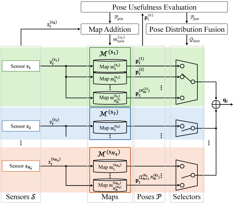
MSMS: Multiplexing sensors and maps system
1. Introduction
Because autonomous mobile robots rely on pose information for fundamental technologies such as mapping, path planning, and obstacle avoidance 1,2,3,4,5,6,7,8, localization, which estimates a robot’s pose from sensor observations, is essential. The mainstream localization methods are map-based approaches 9,10,11,12,13,14,15,16,17,18, which estimate the current robot’s pose by matching current features observed using LiDAR or cameras with a pre-constructed map. Therefore, the robustness of map-based localization should be improved to enable the stable navigation of autonomous mobile robots.
However, because of the environmental dependency of sensors resulting from their sensing principles, each sensor has environments in which the localization accuracy degrades. For example, LiDAR may fail to provide reliable localization in large open spaces or long monotonous corridors where distinctive geometric features are difficult to obtain 19. Cameras may struggle with localization in environments where image features are difficult to extract, such as dark areas 20. Therefore, robust localization is difficult to achieve using a single sensor. To address the environmental dependency of sensors, scholars have proposed multiplexing methods that fuse information from multiple sensors 21,22,23,24,25,26,27,28,29,30. These sensor multiplexing methods include filtering-based fusion 21,22,23,24, optimization-based fusion 25,26, and selective fusion 27,28.
However, localization robustness is degraded not only by the environmental dependency of sensors but also by the condition dependency of maps. Maps represent observed environmental features under the conditions at the time of map construction, and therefore have condition dependency. Because condition changes alter the observed environmental features, the currently observed features no longer match the pre-constructed map, resulting in degraded localization accuracy. LiDAR uses the surrounding geometry for localization. Therefore, for example, when a door state changes from open to closed, the surrounding geometry changes, and reliable localization may no longer be possible 31. Cameras use the features extracted from images. Therefore, for example, when the condition changes from day to night, the extracted features change, and localization may fail 32. Map multiplexing methods that select an appropriate map according to the current conditions have been proposed to address the condition dependency of maps 33,34,35,36,37,38,39. Existing map multiplexing methods include methods that select maps based on the likelihood between the observation model predicted from each map and the current LiDAR observation 33,34, those based on the matching quality between image features and maps 36, and those based on pose information obtained from each map 39.
Robust localization can be achieved against the environmental dependency of sensors by multiplexing sensors and against the condition dependency of maps by multiplexing maps. However, in actual environments, both dependencies coexist, and multiplexing only sensors or maps is insufficient to achieve robust localization against both. Therefore, a system capable of such robust localization is required.
In this paper, we propose a system that multiplexes both sensors and maps, called the multiplexing sensors and maps system (MSMS), to achieve robust localization against the environmental dependency of sensors and the condition dependency of maps. Existing sensor multiplexing and map multiplexing methods cannot be directly applied to the MSMS.
The MSMS is achieved by extending the sensor-agnostic map selection method 39. This method selects the most appropriate map from multiple maps of a single sensor based on the pose usefulness. However, because the MSMS also addresses the environmental dependency of sensors, it multiplexes not only the maps but also the sensors. Therefore, a framework is required to fuse the representative poses obtained from each sensor. Furthermore, sensors that fail to provide useful poses because of their environmental dependency must be excluded from the fusion. In addition, the sensor-agnostic map selection method assumes that the multiplexing of maps suitable for the environment has been prepared in advance. However, in practical operations, the conditions that may be encountered are highly diverse, and creating multiplex maps suitable for the environment in advance to comprehensively cover future conditions is difficult. Therefore, to maintain appropriate maps for each sensor, the MSMS must add new maps when existing ones are insufficient.
The objective of the MSMS is not to develop a single effective localization method. Rather, it was designed to establish a framework that incorporates existing localization methods with different characteristics and achieves robust localization by enabling these methods to complement each other in scenarios where individual methods perform poorly. The experiments in this study focused on validating the effectiveness of the MSMS framework. Therefore, we assumed that at least one correct localization result is included among the multiple localization sources and the proprioceptive sensor observations used to calculate the localization selection metric are reliable. This assumption was adopted to isolate the effect of the proposed framework and evaluate whether the MSMS can correctly select and integrate the localization results obtained from existing methods, as well as appropriately add maps when necessary. Under these assumptions, the objective was to verify that the MSMS framework, which multiplexes both sensors and maps and is fundamentally different from conventional localization approaches, functions as intended and contributes to improving localization robustness. The experimental results demonstrated that the MSMS achieves robust localization against both the environmental dependency of sensors and the condition dependency of maps. The contributions of this study are as follows.
-
・
We developed the MSMS, a framework that multiplexes sensors and maps.
-
・
We developed a mechanism for dynamically adding maps when existing maps are insufficient.
-
・
We demonstrated that the MSMS achieves robustness against the environmental dependency of sensors and the condition dependency of maps.
3. Method
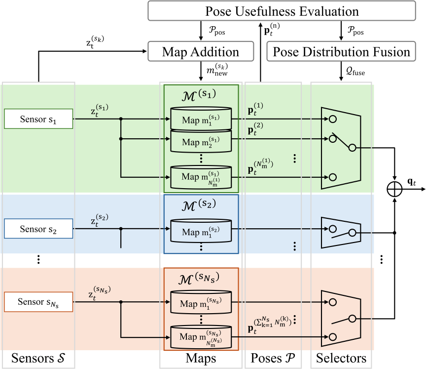
Fig. 1. MSMS. The MSMS consists of the pose-usefulness evaluation, pose fusion, and map addition modules.
In this study, we extend the sensor-agnostic map-selection method39 and propose the MSMS. The MSMS structure is shown in Fig. 1. Let the set of sensors be denoted by \(\mathcal{S}=\{s_1,s_2,\ldots,s_{N_\mathrm{s}}\}\). As shown in Fig. 1, sensors \(s_1, s_2, \ldots,\) and \(s_{N_\mathrm{s}}\) are multiplexed. \(N_\mathrm{s}\) denotes the number of sensors. Each sensor \(s_k \in \mathcal{S}\) has a set of maps \(\mathcal{M}^{(s_k)}=\{m_1^{(s_k)},m_2^{(s_k)},\ldots,m_{N_\mathrm{m}^{(k)}}^{(s_k)}\}\). For each sensor \(s_k\), maps \(m_1^{(s_k)}, m_2^{(s_k)}, \ldots,\) and \(m_{N_\mathrm{m}^{(k)}}^{(s_k)}\) are multiplexed. \(N_\mathrm{m}^{(k)}\) denotes the number of maps for sensor \(s_k\). Let the set of poses obtained by multiplexing the sensors and maps be denoted by \(\mathcal{P}=\{\mathbf{p}^{(n)}_t \mid n=1,2,\ldots,\sum_{k=1}^{N_\mathrm{s}} N_\mathrm{m}^{(k)}\}\). In this paper, the pose \(\mathbf{p}_t^{(n)}\) is defined as a three-dimensional vector \([x,\; y,\; \mathrm{yaw}]^\top\) representing the robot’s absolute pose, where \(\mathbf{p}_t^{(n)}\) is a representative value obtained from the probability distribution \(\mathbf{q}_t^{(n)}\) estimated by each algorithm.
The MSMS consists of the following three modules, which are executed in the following order.
-
1.
Pose-Usefulness Evaluation Module This module determines whether each pose \(\mathbf{p}^{(n)}_t\) in \(\mathcal{P}\) is useful for achieving robust localization. By classifying \(\mathcal{P}\) into a useful pose set \(\mathcal{P}_{\mathrm{pos}}\) and a non-useful pose set \(\mathcal{P}_{\mathrm{neg}}\), and updating them over time, pose usefulness is evaluated over time.
-
2.
Pose Distribution Fusion Module This module determines the poses that should be fused based on the results of the pose-usefulness evaluation module. This determines the most useful pose for each sensor and fuses them. If not all poses obtained from a sensor are useful, the pose distribution of the sensor is not used.
-
3.
Map Addition Module This module adds a new map when the correct localization cannot be achieved using the map set \(\mathcal{M}^{(s)}\) of sensor \(s\). If all poses obtained from a sensor continue to be considered as non-useful for a certain period, a new map is constructed from the observation data during that period and added. If map construction fails, the sensor is considered to be unable to provide a useful pose because of the environmental dependency of the sensors, and no map is added.
In the pose-usefulness evaluation and pose fusion modules, we use two pose-usefulness evaluation indicators that were effective for sensor-agnostic map selection 39. The following sections describe the two pose-usefulness evaluation indicators and three modules.
3.1. Computation of the Two Pose-Usefulness Evaluation Indicators
In this section, we describe the computation of the following two pose-usefulness evaluation indicators used in the MSMS at time \(t\).
-
・
Absolute pose difference \(e_{\mathrm{abs},t}^{(n1,n2)}\) between poses \(\mathbf{p}^{(n1)}_t\) and \(\mathbf{p}^{(n2)}_t\).
-
・
Relative pose difference \(e_{\mathrm{rel},t}^{(n)}\) between pose \(\mathbf{p}^{(n)}_t\) and proprioceptive-sensor pose \(\mathbf{p}^{(\mathrm{pro})}_t\).
\(e_{\mathrm{abs},t}^{(n1,n2)}\) and \(e_{\mathrm{rel},t}^{(n)}\) of \(\mathbf{p}^{(n)}_t\) are computed using Eqs. (1) and (2), respectively.
In Eq. (1), \(e_{\mathrm{abs},t}^{(n1,n2)}\) is obtained by computing the Euclidean distance between \(\mathbf{p}^{(n1)}_t\) and \(\mathbf{p}^{(n2)}_t\) on the \(x\)-\(y\) plane. In Eq. (2), \(e_{\mathrm{rel},t}^{(n)}\) is computed as a weighted sum, with \(\alpha \in [0,1]\), of the translational and rotational difference, based on the mean relative poses \(\delta \mathbf{p}^{(n)}_t\) and \(\delta \mathbf{p}^{(\mathrm{pro})}_t\). These mean relative poses are obtained by applying a time-series moving-average filter to the relative poses of \(\mathbf{p}^{(n)}_t\) and \(\mathbf{p}^{(\mathrm{pro})}_t\), as follows:
3.2. Pose-Usefulness Evaluation Module
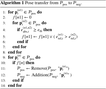
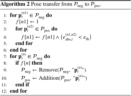
In this section, we describe the updating of the useful pose set \(\mathcal{P}_{\mathrm{pos}}\) and non-useful pose set \(\mathcal{P}_{\mathrm{neg}}\). This process is executed after time step \(w\), considering the window size of the time-series mean filter \(w\). In the initial state (\(t=0\)), all poses \(\mathbf{p}_t^{(n)}\) are included in \(\mathcal{P}_{\mathrm{pos}}\). Here, \(f[n]\) denotes a flag array whose elements are either 0 or 1.
Using Algorithm 1, \(\mathcal{P}_{\mathrm{pos}}\) is updated. Whether the pose \(\mathbf{p}_t^{(n1)}\) in \(\mathcal{P}_{\mathrm{pos}}\) should be moved to \(\mathcal{P}_{\mathrm{neg}}\) is determined by evaluating \(e_{\mathrm{abs},t}^{(n1,n2)}\) with respect to all poses \(\mathbf{p}_t^{(n2)}\) in \(\mathcal{P}_{\mathrm{pos}}\). If a pose \(\mathbf{p}_t^{(n2)}\) exists for which \(e_{\mathrm{abs},t}^{(n1,n2)}\) exceeds \(e_{\mathrm{th}}\), then a localization error is considered to have occurred in either \(\mathbf{p}_t^{(n1)}\) or \(\mathbf{p}_t^{(n2)}\). If \(e_{\mathrm{rel},t}^{(n1)}\) is greater than \(e_{\mathrm{rel},t}^{(n2)}\), \(\mathbf{p}_t^{(n1)}\) is considered to contain a localization error and is moved from \(\mathcal{P}_{\mathrm{pos}}\) to \(\mathcal{P}_{\mathrm{neg}}\).
Next, using Algorithm 2, \(\mathcal{P}_{\mathrm{neg}}\) is updated. Whether the pose \(\mathbf{p}_t^{(n1)}\) in \(\mathcal{P}_{\mathrm{neg}}\) should be returned to \(\mathcal{P}_{\mathrm{pos}}\) is determined by evaluating \(e_{\mathrm{abs},t}^{(n1,n2)}\) with respect to all poses \(\mathbf{p}_t^{(n2)}\) in \(\mathcal{P}_{\mathrm{pos}}\). If all \(e_{\mathrm{abs},t}^{(n1,n2)}\) values are less than \(e_{\mathrm{th}}\), \(\mathbf{p}_t^{(n1)}\) is considered the correct pose and is moved from \(\mathcal{P}_{\mathrm{neg}}\) to \(\mathcal{P}_{\mathrm{pos}}\).
3.3. Pose Distribution Fusion Module
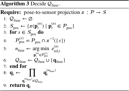
In this section, the pose set for fusion \(\mathcal{Q}_{\mathrm{fuse}}\) is determined from \(\mathcal{P}_{\mathrm{pos}}\) at time \(t\), and the fused probability distribution \(\mathbf{q}_t\) is computed by fusing the poses in \(\mathcal{Q}_{\mathrm{fuse}}\). Using Algorithm 3, a representative pose is determined for each sensor from \(\mathcal{P}_{\mathrm{pos}}\), and fusion is performed by excluding the sensors whose poses are not included in \(\mathcal{P}_{\mathrm{pos}}\).
First, \(\mathcal{Q}_{\mathrm{fuse}}\) is initialized as an empty set. Next, using the mapping \(\pi\), each pose \(\mathbf{p}_t^{(n)}\) in \(\mathcal{P}_{\mathrm{pos}}\) is associated with the sensor that generated it. Consequently, a set of useful sensors \(\mathcal{S}_{\mathrm{pos}}\) is obtained as the set of sensors that generate at least one useful pose.
A representative pose is then determined for each sensor \(s\) in \(\mathcal{S}_{\mathrm{pos}}\). Each \(\mathbf{p}_t^{(n)}\) included in \(\mathcal{P}_{\mathrm{pos}}^{(s)}\) (\(=\mathcal{P}_{\mathrm{pos}}\cap \pi^{\tiny -1}\!\left({s}\right))\) is a useful pose obtained from sensor \(s\). Among them, the \(\mathbf{p}_t^{(n)}\) that minimizes \(e_{\mathrm{rel},t}^{(n)}\) is selected as the representative pose \(\mathbf{q}_t^{(n_{\mathrm{fuse}})}\) for sensor \(s\). Subsequently, the selected \(\mathbf{q}_t^{(n_{\mathrm{fuse}})}\) is added to \(\mathcal{Q}_{\mathrm{fuse}}\). Through the application of this process to all the sensors in \(\mathcal{S}_{\mathrm{pos}}\), sensors that do not provide useful poses can be excluded from the fusion, whereas one useful pose is selected from each sensor that does provide a useful pose.
The final probability distribution \(\mathbf{q}_t\) is obtained by multiplicatively fusing the pose \(\mathbf{q}_t^{(n_{\mathrm{fuse}})}\) in \(\mathcal{Q}_{\mathrm{fuse}}\).
3.4. Map Addition Module
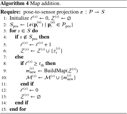
This section describes scenarios in which a new map is added. For a sensor \(s\), if all poses from that sensor continue to be excluded from the useful pose set \(\mathcal{P}_{\mathrm{pos}}\) for a certain period, localization with sensor \(s\) is difficult using the current map set \(\mathcal{M}^{(s)}\), and a new map is constructed and added to the map set \(\mathcal{M}^{(s)}\).
Algorithm 4 is used to determine whether a new map should be added to the map set \(\mathcal{M}^{(s)}\) of sensor \(s\), and if necessary, a new map should be added. First, using the mapping \(\pi\), each pose \(\mathbf{p}_t^{(n)}\) in \(\mathcal{P}_{\mathrm{pos}}\) is associated with the sensor that generated it. Consequently, a set of useful sensors \(\mathcal{S}_{\mathrm{pos}}\) is obtained as the set of sensors that generate at least one useful pose.
Next, for each sensor \(s\) in \(\mathcal{S}\), we determine whether \(s\) is included in the useful sensor set \(\mathcal{S}_{\mathrm{pos}}\). If \(s \notin \mathcal{S}_{\mathrm{pos}}\), the current map set \(\mathcal{M}^{(s)}\) for sensor \(s\) is considered insufficient for accurate localization. At this time, the counter \(\ell^{(s)}\), which represents the duration for which sensor \(s\) has not been classified into a useful sensor set \(\mathcal{S}_{\mathrm{pos}}\), is incremented. In addition, the current observation \(z_t^{(s)}\) is added to the observation buffer \(\mathcal{Z}^{(s)}\) such that observations during that period can later be used for map construction.
However, if \(s \in \mathcal{S}_{\mathrm{pos}}\), the current map set \(\mathcal{M}^{(s)}\) for sensor \(s\) is determined to be sufficient for the correct localization. If the counter \(\ell^{(s)}\) exceeds the threshold \(t_{\mathrm{th}}\), in the environment during that period, correct localization cannot be achieved using the current map set \(\mathcal{M}^{(s)}\) of sensor \(s\). Therefore, using the observation buffer \(\mathcal{Z}^{(s)}\), a new map is constructed and added to the map set \(\mathcal{M}^{(s)}\) of sensor \(s\). Finally, when sensor \(s\) can localize correctly, the counter \(\ell^{(s)}\) is reset to 0 and \(\mathcal{Z}^{(s)}\) is initialized as an empty set.
4. Experiments Using LILocBench Datasets
4.1. Experimental Overview
The LILocBench dataset evaluates long-term localization performance in indoor environments where condition changes occur. It was collected in a real-world environment 40. In this dataset, data labeled as static and long-term changes (hereafter, lt_changes) were used. Static data represent static environments or static environments in which natural changes may occur in daily life, such as slight chair or human movements. The lt_changes data represent environments in which condition changes, such as the appearance or rearrangement of cardboard boxes and furniture and the opening and closing of doors, occur relative to the static environments. In this dataset, the data were collected in an indoor environment, as shown in Fig. 2(a) using the robot shown in Fig. 2(b). The robot platform is based on an omnidirectional mobile robot (Clearpath Robotics Dingo) equipped with two 2D LiDARs (SICK TIM781S) and three RGB-D cameras (Intel RealSense D455). In this experiment, the front 2D LiDAR (blue), the rear 2D LiDAR (green), the front RGB-D camera (red), and wheel odometry as proprioceptive sensors were used. For the localization methods, Cartographer 41 was used for the 2D LiDARs, and ORBSLAM2 42 was used for the RGB-D camera. The parameters used in this experiment were \(\alpha=0.8\), \(\omega=100\), \(e_{\mathrm{th}}=0.5\), and \(t_{\mathrm{th}}=25\).
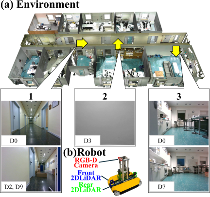
Fig. 2. Experimental environment and robot.
| Data | Data label | Description |
| D0 | static_0 | Static environment. |
| D1 | static_2 | Static environment. |
| D2 | lt_changes_5 | Environment including object arrangements completely inconsistent with the static environment. |
| D3 | static_4 | Static environment. |
| D4 | lt_changes_3 | Environment in which the doors of all rooms were closed. |
| D5 | static_1 | Static environment. |
| D6 | static_6 | Static environment including natural changes. |
| D7 | lt_changes_1 | Environment with rearranged furniture and placed cardboard boxes. |
| D8 | static_5 | Static environment including natural changes. |
| D9 | lt_changes_4 | Environment including object arrangements completely inconsistent with the static environment. |
| D10 | static_3 | Static environment. |
| D11 | lt_changes_2 | Environment in which cardboard boxes were placed. |
| D12 | lt_changes_0 | Environment with rearranged furniture and placed cardboard boxes. |
The 13 datasets used in the experiments (static_0–static_6 and lt_changes_0–lt_changes_5) were assigned to D0–D12, as listed in Table 1. Because D0 was used to construct the initial map, it was set to static_0, which covered the entire environment and corresponded to a static environment.
The initial maps for the 2D LiDARs and RGB-D camera were constructed using D0, and localization was performed on D1–D12. In this experiment, the ground truth (gt) was defined as the localization using the integrated point clouds of the front and rear 2D LiDARs using a map constructed from the same data used for localization.
4.2. Experimental Results
4.2.1. Map Configurations for Each Run
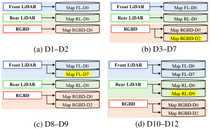
Fig. 3. Map configurations for each dataset.
-
1.
D1–D2 In D1–D2, localization was performed using the map configuration shown in Fig. 3(a), which corresponds to the initial state. In D1, no map addition was deemed necessary. In D2, map addition was deemed necessary for the RGB-D camera. Therefore, Map RGBD-D2 was added to the map set of the RGB-D camera for subsequent localization. This was caused by the appearance of cardboard boxes and partitions in the corridor in D2 compared with D0, in which the initial map was constructed, as indicated by callout 1 in Fig. 2.
-
2.
D3–D7 In D3–D7, localization was performed using the map configuration shown in Fig. 3(b). In D7, map addition was deemed necessary for the front 2D LiDAR. Therefore, Map FL-D7 was added to the map set of the front 2D LiDAR for subsequent localization. This was caused by the change in the room layout in D7 compared with D0, in which the initial map was constructed, as indicated by callout 3 in Fig. 2.
-
3.
D8–D9 In D8 and D9, localization was performed using the map configuration shown in Fig. 3(c). In D9, map addition was deemed necessary for the rear 2D LiDAR. Therefore, Map RL-D9 was added to the map set of the rear 2D LiDAR for subsequent localization. This was caused by the appearance of cardboard boxes and partitions in the corridor in D9 compared with D0, in which the initial map was constructed, as indicated by callout 1 in Fig. 2.
-
4.
D10–D12 In D10–D12, localization was performed using the map configuration shown in Fig. 3(d). In D12, we determined that a new map must be added.
4.2.2. Evaluation of Localization Robustness
| Data | Proposed |
Map FL-D0 |
Map RL-D0 |
Map RGBD-D0 |
| D1 |
1.00 0.114 0.080 |
1.00 0.122 0.076 |
1.00 0.141 0.086 |
0.93 0.733 0.224 |
| D2 |
1.00 0.177 0.061 |
1.00 0.164 0.075 |
1.00 0.235 0.065 |
0.63 0.471 0.160 |
| D3 |
1.00 0.099 0.036 |
1.00 0.063 0.021 |
1.00 0.110 0.050 |
0.87 0.781 0.259 |
| D4 |
1.00 0.132 0.037 |
1.00 0.075 0.022 |
1.00 0.198 0.050 |
0.90 0.499 0.147 |
| D5 |
1.00 0.142 0.046 |
1.00 0.095 0.037 |
1.00 0.133 0.059 |
0.97 0.474 0.176 |
| D6 |
1.00 0.145 0.048 |
1.00 0.145 0.066 |
1.00 0.205 0.047 |
0.96 0.540 0.167 |
| D7 |
1.00 0.274 0.105 |
1.00 8.443 0.739 |
1.00 0.291 0.112 |
0.84 0.723 0.156 |
| D8 |
1.00 0.091 0.045 |
1.00 0.098 0.038 |
1.00 0.116 0.056 |
0.99 0.242 0.134 |
| D9 |
1.00 0.240 0.067 |
1.00 11.770 0.295 |
1.00 3.723 0.202 |
0.75 0.797 0.208 |
| D10 |
1.00 0.172 0.078 |
1.00 0.120 0.062 |
1.00 0.172 0.087 |
0.94 0.749 0.220 |
| D11 |
1.00 0.200 0.060 |
1.00 0.289 0.052 |
1.00 0.130 0.046 |
0.99 0.479 0.167 |
| D12 |
1.00 0.467 0.079 |
0.99 1.801 0.127 |
1.00 8.035 0.260 |
0.84 0.335 0.132 |
The robustness of the localization was evaluated by comparing four localization sources on D1–D12: the proposed system and three initial maps, namely Maps FL-D0, RL-D0, and RGBD-D0.
Table 2 lists the completion rate (ratio of time steps for which pose information is available), maximum localization error, and average localization error of the proposed system and Maps FL-D0, RL-D0, and RGBD-D0 for D1–D12. From top to bottom, the values in each cell represent the completion rate, maximum localization error, and average localization error.
Focusing on the completion rate, the proposed system, Map FL-D0, and Map RL-D0 did not experience any localization failures (no pose information was available) even once over all 12 datasets. Note that the value of Map FL-D0 in D12 was 0.99 because the initial localization took somewhat longer, during which the pose information could not be obtained. In contrast, for Map RGBD-D0, localization failures caused by motion blur owing to robot rotation, condition changes, and white walls were confirmed in all 11 run datasets except for D8. The value of Map RGBD-D0 in D8 was 0.99 because the initial localization was somewhat longer.
| Method | MLE [m] | ALE [m] |
|
Map FL-D0 (D1, D3, D5, D10) |
0.063–0.122 | 0.021–0.076 |
|
Map RL-D0 (D1, D3, D5, D10) |
0.110–0.172 | 0.050–0.087 |
|
Map RGBD-D0 (D1, D3, D5, D10) |
0.474–0.781 | 0.176–0.259 |
|
Proposed (D1–D12) |
0.091–0.467 | 0.036–0.105 |
Next, the robustness of the localization was examined from the perspectives of the maximum and average localization errors. In this experiment, the localization errors obtained in D1, D3, D5, and D10, which were the same environments used to construct Maps FL-D0, RL-D0, and RGBD-D0, were used as reference values to evaluate the localization robustness. Table 3 summarizes the ranges of the maximum and average localization errors for the proposed method (D1–D12) and for Maps FL-D0, RL-D0, and RGBD-D0 (D1, D3, D5, and D10), based on the results presented in Table 2.
Focusing on the maximum localization error in Table 2, large localization errors were confirmed for Map FL-D0 in D7, D9, and D12, i.e., 8.443, 11.770, and 1.801 m, respectively, and for Map RL-D0 in D9 and D12, namely 3.723 m and 8.035 m, respectively. In contrast, as shown in Table 3, the maximum localization errors of the proposed method over D1–D12 ranged from 0.091 to 0.467 m. Although these values were slightly larger than those of the reference 2D LiDAR-based localization methods in the reference environments, the proposed method maintained bounded localization errors over all datasets, including environments where large localization errors were observed for individual localization sources. Furthermore, all maximum localization errors remained below the robot dimensions (front-back direction: 0.686 m, left-right direction: 0.517 m), indicating that they were unlikely to cause hazardous scenarios such as collisions.
Next, focusing on the average localization error in Table 3, the proposed method achieved average localization errors ranging from 0.036 m to 0.105 m over D1–D12. As shown in Table 3, these values indicated that the proposed method maintained a stable localization performance over all datasets, demonstrating robustness against the environmental dependency of sensors and the condition dependency of maps.
These results confirmed that the proposed system achieved robust localization against the environmental dependency of sensors and the condition dependency of maps over all datasets while maintaining localization availability and bounded localization errors.
4.2.3. Case with the Environmental Dependency of Sensors
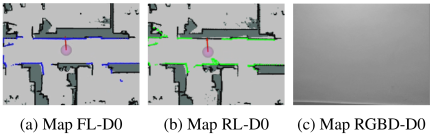
Fig. 4. Localization in D3.
In D3, as shown in Fig. 2, feature points could not be obtained from the camera images in a certain period because of a white wall, and RGB-D camera localization (Map RGBD-D0 (Fig. 4(c)), Map RGBD-D2) failed. Fig. 4(c) shows the ORB-SLAM2 debugging view, confirming that visual tracking was lost during this period. During this period, Maps FL-D0 and RL-D0 could perform localization because the maps and observations are appropriately matched, as shown in Figs. 4(a) and (b). Here, the maps represent occupancy grid maps, where the black regions indicate occupied cells corresponding to environmental structures, whereas the observations represent LiDAR point clouds shown in blue or green. Thus, robust localization was achieved against the environmental dependency of the RGB-D camera by complementing it with the front and rear 2D LiDARs.
4.2.4. Case with the Condition Dependency of Maps
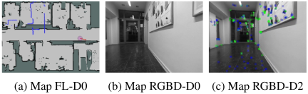
Fig. 5. Localization in D9.
In D9, as shown in Fig. 2, condition changes occurred compared with D0, in which the initial map was constructed, such as the appearance of cardboard boxes and partitions in the corridor. In this environment, the front 2D LiDAR (Map FL-D0 (Fig. 5(a)), Map FL-D7) and rear 2D LiDAR (Map RL-D0) incorrectly matched the map and observations, causing large localization errors. Here, the maps represent occupancy grid maps, where the black regions indicate occupied cells corresponding to environmental structures, whereas the observations represent LiDAR point clouds shown in blue. In addition, for the RGB-D camera (Map RGBD-D0 (Fig. 5(b))), the map and observations did not match, and localization failed. However, in this environment, the RGB-D camera (Map RGBD-D2) was appropriately matched to the map and observations, as shown in Fig. 5(c), and localization was possible. Although no tracked feature points are observed in Fig. 5(b), numerous matched feature points (shown in green) are visible in Fig. 5(c), indicating successful matching between the observations and the map.
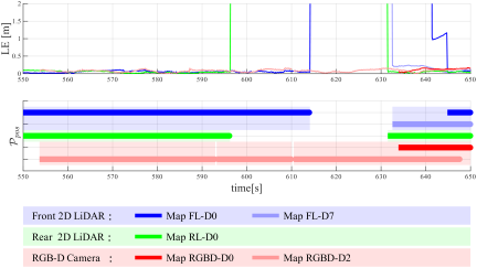
Fig. 6. Time-series data of the LE and \(\mathcal{P}_{\mathrm{pos}}\) in D9.
The time-series data of the localization error (LE) and \(\mathcal{P}_{\mathrm{pos}}\) in D9, shown in Fig. 6, also confirmed that the map addition module in the MSMS contributes to robust localization against the condition dependency of maps. As described above, large localization errors were observed for the front 2D LiDAR (Maps FL-D0 and FL-D7) and rear 2D LiDAR (Map RL-D0). In addition, the LE plot for the RGB-D camera (Map RGBD-D0) was interrupted, indicating a localization failure. The MSMS was used to detect these unreliable results and exclude them from \(\mathcal{P}_{\mathrm{pos}}\). Meanwhile, during the period in which Maps FL-D0, FL-D7, RL-D0, and RGBD-D0 were not useful, the RGB-D camera (Map RGBD-D2) was classified as \(\mathcal{P}_{\mathrm{pos}}\). During this period, Map RGBD-D2 achieved accurate localization, indicating that the RGB-D camera map added to D2 was effectively utilized.
Thus, the maps dynamically added by the map addition module enabled robust localization against the condition dependency of the maps.
5. Conclusion
To achieve robust localization against the environmental dependency of sensors and condition dependency of maps, we propose the MSMS. It consists of pose-usefulness evaluation, pose fusion, and map addition modules. The pose usefulness evaluation module determines the usefulness of the pose information obtained through sensor and map multiplexing. The pose fusion module determines which pose information should be fused based on the pose usefulness and computes the final estimated pose, thereby achieving stable localization. The map addition module adds a new map when all poses obtained from a sensor’s map set are deemed not useful, thereby enabling localization when the same conditions are encountered again. Through experiments using a dataset, the proposed system consistently achieved robust localization by complementing sensors with different characteristics to address the environmental dependency of sensors and by using added maps to address the condition dependency of maps.
Future studies should pursue the following three major directions. First, the assumptions adopted in this study should be relaxed. In this study, we assumed that at least one correct localization result exists among the available localization sources and that the proprioceptive sensor observations used for localization selection are reliable. Future studies should focus on relaxing these assumptions. Regarding the first assumption, the characteristics and applicable conditions of existing localization methods should be investigated in detail, and combinations of complementary methods that can cover as wide a range of environments and time periods as possible should be identified, such that at least one method remains effective. Regarding the second assumption, the reliability and robustness of the localization selection metric should be improved by integrating multiple proprioceptive sensors and incorporating existing odometry estimation methods based on exteroceptive sensors.
Second, map management should be addressed from the perspective of computational efficiency in practical applications. Although this study focused on a map addition framework, continuous map addition increases the number of maintained maps, which may result in increased computational costs during localization. Therefore, future studies should investigate map-management strategies, including the removal or integration of unnecessary maps. Furthermore, as the environmental region associated with each map can be identified during map construction, the computational cost can be reduced by dynamically selecting maps based on the current operating region. Other important aspects include imposing an upper limit on the number of maps maintained for each sensor and selecting localization algorithms that achieve a suitable balance between the computational cost and number of maps. Addressing these challenges is expected to improve the applicability and real-time performance of the MSMS in real-world environments.
Third, further comprehensive evaluations should be conducted under various environments and conditions. The generalization capability of the proposed framework was evaluated using a limited dataset. Therefore, future studies should conduct experiments using real-world datasets collected from various indoor and outdoor environments, including diverse sensor environmental and map condition dependencies. In addition, the computational cost, scalability, and real-time performance should be evaluated under different operating environments, sensor configurations, and localization algorithms because these factors are highly dependent on the experimental conditions. Such evaluations will provide a more comprehensive understanding of the applicability and limitations of MSMS in real-world environments.
- [1] J. Graeter, A. Wilczynski, and M. Lauer, “Limo: Lidar-monocular visual odometry,” 2018 IEEE/RSJ Int. Conf. on Intelligent Robots and Systems (IROS), pp. 7872-7879, 2018. https://doi.org/10.1109/IROS.2018.8594394
- [2] S. Khan, D. Wollherr, and M. Buss, “Modeling laser intensities for simultaneous localization and mapping,” IEEE Robotics and Automation Letters, Vol.1, No.2, pp. 692-699, 2016. https://doi.org/10.1109/LRA.2016.2516592
- [3] J. Biswas and M. Veloso, “Depth camera based indoor mobile robot localization and navigation,” 2012 IEEE Int. Conf. on Robotics and Automation, pp. 1697-1702, 2012. https://doi.org/10.1109/ICRA.2012.6224766
- [4] J. A. Castellanos, J. Neira, and J. D. Tardós, “Multisensor fusion for simultaneous localization and map building,” IEEE Trans. on Robotics and Automation, Vol.17, No.6, pp. 908-914, 2001. https://doi.org/10.1109/70.976024
- [5] H. T. Niknejad, M. Seiichi, H. Long, and H. Quoc, “Multi-sensor data fusion for autonomous vehicle navigation and localization through precise map,” Int. J. of Automotive Engineering, Vol.3, No.1, pp. 19-25, 2012. https://doi.org/10.20485/jsaeijae.3.1_19
- [6] T. Shan and B. Englot, “Lego-loam: Lightweight and ground-optimized lidar odometry and mapping on variable terrain,” 2018 IEEE/RSJ Int. Conf. on Intelligent Robots and Systems (IROS), pp. 4758-4765, 2018. https://doi.org/10.1109/IROS.2018.8594299
- [7] B. Yang and R. Yang, “Interactive particle filter with occlusion handling for multi-target tracking,” 2015 12th Int. Conf. on Fuzzy Systems and Knowledge Discovery (FSKD), pp. 1945-1949, 2015. https://doi.org/10.1109/FSKD.2015.7382246
- [8] A. Bajcsy, S. L. Herbert, D. Fridovich-Keil, J. F. Fisac, S. Deglurkar, A. D. Dragan, and C. J. Tomlin, “A scalable framework for real-time multi-robot, multi-human collision avoidance,” 2019 Int. Conf. on Robotics and Automation (ICRA), pp. 936-943, 2019. https://doi.org/10.1109/ICRA.2019.8794457
- [9] H. Liu, H. Huang, S.-K. Yeung, and M. Liu, “360ST-Mapping: An Online Semantics-Guided Topological Mapping Module for Omnidirectional Visual SLAM,” 2022 IEEE/RSJ Int. Conf. on Intelligent Robots and Systems (IROS), pp. 802-807, 2022. https://doi.org/10.1109/IROS47612.2022.9982142
- [10] J. Wang, B. Tian, R. Zhang, and L. Chen, “ULSM: Underground Localization and Semantic Mapping with Salient Region Loop Closure under Perceptually-Degraded Environment,” 2022 IEEE/RSJ Int. Conf. on Intelligent Robots and Systems (IROS), pp. 1320-1327, 2022. https://doi.org/10.1109/IROS47612.2022.9982170
- [11] R. Long, C. Rauch, T. Zhang, V. Ivan, T. L. Lam, and S. Vijayakumar, “RGB-D SLAM in Indoor Planar Environments with Multiple Large Dynamic Objects,” IEEE Robotics and Automation Letters, Vol.7, No.3, pp. 8209-8216, 2022. https://doi.org/10.1109/LRA.2022.3186091
- [12] Y. Wang, K. Xu, Y. Tian, and X. Ding, “DRG-SLAM: A Semantic RGB-D SLAM Using Geometric Features for Indoor Dynamic Scene,” 2022 IEEE/RSJ Int. Conf. on Intelligent Robots and Systems (IROS), pp. 1352-1359, 2022. https://doi.org/10.1109/IROS47612.2022.9981238
- [13] K. Gunji, K. Ohno, S. Kojima, R. Bezerra, Y. Okada, M. Konyo, and S. Tadokoro, “LayoutSLAM: Object Layout based Simultaneous Localization and Mapping for Reducing Object Map Distortion,” 2022 IEEE/RSJ Int. Conf. on Intelligent Robots and Systems (IROS), pp. 2825-2832, 2022. https://doi.org/10.1109/IROS47612.2022.9981492
- [14] A. Papadimitriou, I. Kleitsiotis, I. Kostavelis, I. Mariolis, D. Giakoumis, S. Likothanassis, and D. Tzovaras, “Loop Closure Detection and SLAM in Vineyards with Deep Semantic Cues,” 2022 Int. Conf. on Robotics and Automation (ICRA), pp. 2251-2258, 2022. https://doi.org/10.1109/ICRA46639.2022.9812419
- [15] J. Liu, K. Chen, R. Liu, Y. Yang, Z. Wang, and J. Zhang, “Robust and Accurate Multi-Agent SLAM with Efficient Communication for Smart Mobiles,” 2022 Int. Conf. on Robotics and Automation (ICRA), pp. 2782-2788, 2022. https://doi.org/10.1109/ICRA46639.2022.9812366
- [16] Y. Huang, T. Shan, F. Chen, and B. Englot, “DiSCo-SLAM: Distributed Scan Context-Enabled Multi-Robot LiDAR SLAM with Two-Stage Global-Local Graph Optimization,” IEEE Robotics and Automation Letters, Vol.7, No.2, pp. 1150-1157, 2022. https://doi.org/10.1109/LRA.2021.3138156
- [17] M. Frosi and M. Matteucci, “ART-SLAM: Accurate Real-Time 6DoF LiDAR SLAM,” IEEE Robotics and Automation Letters, Vol.7, No.2, pp. 2692-2699, 2022. https://doi.org/10.1109/LRA.2022.3144795
- [18] Z. Liao, Y. Hu, J. Zhang, X. Qi, X. Zhang, and W. Wang, “SO-SLAM: Semantic Object SLAM with Scale Proportional and Symmetrical Texture Constraints,” IEEE Robotics and Automation Letters, Vol.7, No.2, pp. 4008-4015, 2022. https://doi.org/10.1109/LRA.2022.3148465
- [19] A. Zhang and M. M. Atia, “Comparison of 2D localization using radar and LiDAR in long corridors,” 2020 IEEE SENSORS, 2020. https://doi.org/10.1109/SENSORS47125.2020.9278684
- [20] X. Deng, Z. Zhang, A. Sintov, J. Huang, and T. Bretl, “Feature-constrained Active Visual SLAM for Mobile Robot Navigation,” 2018 IEEE Int. Conf. on Robotics and Automation (ICRA), pp. 7233-7238, 2018. https://doi.org/10.1109/ICRA.2018.8460721
- [21] G. Nützi, S. Weiss, D. Scaramuzza, and R. Siegwart, “Fusion of IMU and vision for absolute scale estimation in monocular SLAM,” J. of Intelligent & Robotic Systems, Vol.61, No.1, pp. 287-299, 2011. https://doi.org/10.1007/s10846-010-9490-z
- [22] E. López, R. Barea, A. Gómez, Á. Saltos, L. M. Bergasa, E. J. Molinos, and A. Nemra, “Indoor SLAM for micro aerial vehicles using visual and laser sensor fusion,” Robot 2015: Second Iberian Robotics Conf. pp. 531-542, 2015. https://doi.org/10.1007/978-3-319-27146-0_41
- [23] P. Carrasco, F. Cuesta, R. Caballero, F. J. Perez-Grau, and A. Viguria, “Multi-sensor fusion for aerial robots in industrial GNSS-denied environments,” Applied Sciences, Vol.11, No.9, Article No.3921, 2021. https://doi.org/10.3390/app11093921
- [24] Y. Wang and X. Li, “The IMU/UWB fusion positioning algorithm based on a particle filter,” ISPRS Int. J. of Geo-Information, Vol.6, No.8, Article No.235, 2017. https://doi.org/10.3390/ijgi6080235
- [25] R. Mascaro, L. Teixeira, T. Hinzmann, R. Siegwart, and M. Chli, “GOMSF: Graph-optimization based multi-sensor fusion for robust UAV pose estimation,” 2018 IEEE Int. Conf. on Robotics and Automation (ICRA), pp. 1421-1428, 2018. https://doi.org/10.1109/ICRA.2018.8460193
- [26] Y. Jia, H. Luo, F. Zhao, G. Jiang, Y. Li, J. Yan, Z. Jiang, and Z. Wang, “Lvio-fusion: A self-adaptive multi-sensor fusion SLAM framework using actor-critic method,” 2021 IEEE/RSJ Int. Conf. on Intelligent Robots and Systems (IROS), pp. 286-293, 2021. https://doi.org/10.1109/IROS51168.2021.9635905
- [27] N. Ohashi, Y. Funabora, S. Doki, and K. Doki, “Multisensor robust localization in various environment with correlation checking test,” ROBOMECH J., Vol.8, Article No.3, 2021. https://doi.org/10.1186/s40648-021-00190-9
- [28] T. Suzuki, Y. Funabora, S. Doki, K. Doki, and M. Yamazumi, “DSFS: Dynamic Sensor Fusion System for Robust Localization with Diverse Sensing Information,” J. Robot. Mechatron., Vol.37, No.5, pp. 1127-1136, 2025. https://doi.org/10.20965/jrm.2025.p1127
- [29] J. Lee, M. Ohata, H. Itoh, and E. Morimoto, “LiDAR–Camera Fusion for 3D Fruit Counting and Density Mapping in Horizontal Trellis Orchards,” J. Robot. Mechatron., Vol.38, No.2, pp. 449-459, 2026. https://doi.org/10.20965/jrm.2026.p0449
- [30] S. A. Rahok, R. Onozuka, H. Oneda, K. Inoue, Y. Tokoi, A. Tanaka, and K. Ozaki, “Global and Local Localizations Using an Environmental Magnetic Field and a Scan Matching Method,” J. Robot. Mechatron., Vol.37, No.6, pp. 1365-1373, 2025. https://doi.org/10.20965/jrm.2025.p1365
- [31] D. Avots, E. Lim, R. Thibaux, and S. Thrun, “A probabilistic technique for simultaneous localization and door state estimation with mobile robots in dynamic environments,” IEEE/RSJ Int. Conf. on Intelligent Robots and Systems, pp. 521-526, 2002. https://doi.org/10.1109/IRDS.2002.1041443
- [32] G. Pascoe, W. Maddern, M. Tanner, P. Piniés, and P. Newman, “NID-SLAM: Robust monocular SLAM using normalised information distance,” Proc. of the IEEE Conf. on Computer Vision and Pattern Recognition, pp. 1435-1444, 2017. https://doi.org/10.1109/CVPR.2017.158
- [33] P. Biber and T. Duckett, “Experimental analysis of sample-based maps for long-term SLAM,” The Int. J. of Robotics Research, Vol.28, No.1, pp. 20-33, 2009. https://doi.org/10.1177/0278364908096286
- [34] P. Biber and T. Duckett, “Dynamic maps for long-term operation of mobile service robots,” Proc. of Robotics: Science and Systems (RSS), pp. 17-24, 2005. https://doi.org/10.15607/RSS.2005.I.003
- [35] C. Stachniss and W. Burgard, “Mobile robot mapping and localization in non-static environments,” Proc. of the 20th National Conf. on Artificial Intelligence (AAAI’05) pp. 1324-1329, 2005.
- [36] M. Labbé and F. Michaud, “Multi-session visual SLAM for illumination-invariant re-localization in indoor environments,” Frontiers in Robotics and AI, Vol.9, Article No.801886, 2022. https://doi.org/10.3389/frobt.2022.801886
- [37] C. Linegar, W. Churchill, and P. Newman, “Work smart, not hard: Recalling relevant experiences for vast-scale but time-constrained localisation,” 2015 IEEE Int. Conf. on Robotics and Automation (ICRA), pp. 90-97, 2015. https://doi.org/10.1109/ICRA.2015.7138985
- [38] T. Morris, F. Dayoub, P. Corke, G. Wyeth, and B. Upcroft, “Multiple map hypotheses for planning and navigating in non-stationary environments,” 2014 IEEE Int. Conf. on Robotics and Automation (ICRA), pp. 2765-2770, 2014. https://doi.org/10.1109/ICRA.2014.6907255
- [39] T. Suzuki, Y. Funabora, S. Doki, and K. Doki, “Robust Localization using Map Selection from Multiple Maps Based on the Relative Pose Difference of Map and Interoceptive Sensor,” 2026 IEEE/SICE Int. Symposium on System Integrations (SII2026), 2026. https://doi.org/10.1109/SII64115.2026.11404656
- [40] N. Trekel, T. Guadagnino, T. Läbe, L. Wiesmann, P. Aguiar, J. Behley, and C. Stachniss, “Benchmark for Evaluating Long-Term Localization in Indoor Environments Under Substantial Static and Dynamic Scene Changes,” Proc. of the IEEE/RSJ Int. Conf. on Intelligent Robots and Systems (IROS), 2025. https://doi.org/10.1109/IROS60139.2025.11246416
- [41] W. Hess, D. Kohler, H. Rapp, and D. Andor, “Real-time loop closure in 2D LIDAR SLAM,” 2016 IEEE Int. Conf. on Robotics and Automation (ICRA), pp. 1271-1278, 2016. https://doi.org/10.1109/ICRA.2016.7487258
- [42] R. Mur-Artal and J. D. Tardós, “ORB-SLAM2: An Open-Source SLAM System for Monocular, Stereo, and RGB-D Cameras,” IEEE Trans. on Robotics, Vol.33, No.5, pp. 1255-1262, 2017. https://doi.org/10.1109/TRO.2017.2705103
This article is published under a Creative Commons Attribution-NoDerivatives 4.0 Internationa License.