
Paper:
Target Following for a Snake-Like Robot Using Rolling Locomotion via Deep Reinforcement Learning
Tsuyoshi Kimoto
 , Akio Yamano
, Satomi Suzuki, and Takashi Iwasa
Department of Aerospace Engineering, Graduate School of Engineering, Osaka Metropolitan University
1-1 Gakuen-cho, Naka-ku, Sakai, Osaka 599-8531, Japan

The turning motion of snake-like robots based on center of gravity shift has superior energy efficiency compared to the undulatory locomotion that simultaneously drives many joints, but precise guidance control has been difficult due to its nonlinear dynamic characteristics. In this paper, we propose a control method using deep reinforcement learning for following target points in all directions in the turning motion using center of gravity shift and ground reaction forces. The target direction is defined as a normalized vector in the body coordinate system. This allows us to present target direction information to the agent that is independent of changes in self-orientation, and we show that it can acquire a policy for accurate following in all directions. The results of motion analysis confirmed that the learned policy not only skillfully utilizes the ground reaction forces at the time of contact to make dynamic trajectory corrections, but also achieves target following by flexibly switching the turning strategy according to the target direction.
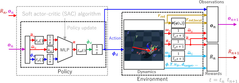
DRL framework for rolling locomotion
1. Introduction
Snake-like robots have robustness and stability, and can move in harsh environments such as narrow spaces, underwater, and uneven terrain where conventional wheeled robots cannot move. Therefore, they are expected to be used in a wide range of tasks such as support in disaster sites 1,2, inspection of pipes and other structures 3,4, work in factories 5, and planetary exploration 6,7.
Many papers have been written about the locomotion of snake-like robots, and most of them are about the undulatory locomotion of snakes. Tesch et al. described the joint angles as a sinusoidal function, which made it possible to generate complex undulatory locomotion of snakes using only a few important parameters 8. This greatly improved operability and simplified user control. Takemori et al. proposed a crawler gait that allows the body of the snake-like robot to act like a large crawler belt, making it easier to adapt to uneven terrain and enabling high-speed movement on uneven terrain 9,10. However, there are still some problems to be solved to make snake-like robots fully functional in uncertain environments. In particular, since many of the snake-like robot’s locomotion modes require the simultaneous driving of many actuators due to their operating principles, energy consumption is large. The problem of energy efficiency is an important issue to be solved.
Examples of searching for an appropriate driving method include Tesch et al., who attempted to find parameters for the undulatory locomotion of a snake-like robot moving on land and simultaneously optimize the stability of the head and the speed of the robot 11. Hasanzadeh and Tootoonchi used a genetic algorithm to find parameters for the undulatory locomotion of a snake-like robot moving on land that can achieve maximum speed while keeping the angle of the head link within a certain range 12. Crespi and Ijspeert used a heuristic optimization algorithm called the Powell method to optimize the running speed of the robot on land, in water, and on slopes 13. In recent years, research combining central pattern generators and deep reinforcement learning (DRL) has been actively conducted as a method that can cope with greater design freedom and feedback of observations from the environment to the motion 14,15,16.
However, the problem of energy efficiency due to the simultaneous driving of many actuators under load still remains, and it is considered difficult to further improve energy efficiency with undulatory locomotion. Furthermore, research on reconfigurable robots that can select locomotion modes according to the environment and improve mobility has been conducted, not limited to optimizing the locomotion of snake-like robots. Such robots can switch between multiple locomotion modes, such as crawling, quadrupedal walking, and rolling locomotion in a loop shape by connecting both ends of the body 17,18,19,20,21,22. In particular, rolling locomotion in a loop shape has a great advantage in terms of locomotion efficiency because it can move quickly on flat ground while suppressing friction with the ground. However, many of these deformation forms still require the continuous driving of many joints to maintain a specific shape, and a single loop shape is prone to tipping over against unevenness of the road surface, and there were also concerns about the risk of mechanical failure due to the intrusion of mud and sand.
Therefore, the authors proposed a new rolling locomotion method based on the principle of center of gravity shift in previous research, aiming for a fundamental improvement in locomotion efficiency and an increase in reliability 23. In this method, the robot is deformed into a tire shape like a parallel two-wheeled vehicle, and propulsion is achieved by utilizing the change in the center of gravity position and the gravitational torque caused by a slight displacement of the head or tail. This propulsion method improves locomotion efficiency and allows for stable running even in environments with unevenness, as it becomes a balanced two-wheeled shape, reducing the risk of tipping over compared to a single loop shape 17,18,19,24,25,26. In addition, it has a practical advantage in that it has an extremely simple shape that can be equipped with a waterproof cover, making it less likely to malfunction in harsh environments such as muddy terrain. However, this rolling locomotion based on center of gravity shift has high efficiency, but its dynamics are nonlinear and difficult to control.
In previous research, we have designed a specific steady joint trajectory using trial and error 23 and a multi-objective genetic algorithm 27, but these were mainly focused on stable running under constant conditions. There is a physical time delay until the change in the center of gravity appears as an actual rolling locomotion. Therefore, control methods for correcting the trajectory when the running direction deviates due to disturbances and for guiding to arbitrary target points have not been established.
In controlling such complex nonlinear systems, optimal control approaches such as model predictive control are one effective means. However, due to the difficulty of modeling and the high computational cost, there are many challenges in ensuring real-time control cycles. DRL is a method that can acquire robust control laws through trial and error in simulation, and has been widely adopted in the field of robot control in recent years. We have shown through simulation and experiments that robust straightness in rolling locomotion can be acquired by DRL with an observation buffer 28,29,30. Furthermore, through experiments in previous research 30, it has been quantitatively shown that this rolling locomotion based on center of gravity shift can reduce the number of simultaneously driven actuators and achieve high locomotion efficiency on smooth floors compared to conventional locomotion (side winding, linear progression, rectilinear progression).
In this study, we establish target-following control (target-reaching task) based on high-efficiency rolling locomotion by center of gravity shift using DRL. By designing a state space that incorporates the target direction as a normalized vector in the body coordinate system, we enable direct learning of the correlation between the robot’s self-orientation and the target position, and we introduce an observation buffer to stabilize learning in systems with time delays as before. We evaluate the effectiveness of the proposed method through simulation and demonstrate that accurate target following is possible. This study is based on a simulation environment calibrated with empirical data from previous research 30, and it is designed with consideration of the motion characteristics of the real environment, so reproducibility is expected in future applications to physical systems.
2. Simulation Model
2.1. Snake-Like Robot
An overview of the proposed snake-like robot is shown in Fig. 1. Other than the body link with an inertial measurement unit (IMU) and a single-board computer (SBC), the structure is the same as the previous research 23,27. The authors proposed a snake-like robot that can switch between undulatory locomotion and rolling locomotion by center of gravity shift. The rolling locomotion is generated by center of gravity shift using the deformation of multiple links, and it is a mode to realize high running efficiency on even ground. Undulatory locomotion such as sidewinding 31,32 and swimming 33,34 have high running performance on uneven terrain and in fluids, but they consume a lot of power.
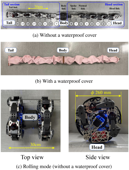
Fig. 1. Overview of the snake-like robot 28,29,30. (a) Without a waterproof cover. The number inside the circle represents the actuator index. (b) With a waterproof cover. (c) Rolling mode.
The specifications of the snake-like robot are shown in Table 1. The total length of the snake-like robot is 1.76 m, the mass is 5.76 kg, and it is a multi-link mechanism in which the axes of 16 actuators (B3M-SC-1170-A, KondoKagaku, Co., Ltd., Japan) are arranged so that they are perpendicular to each other (Fig. 1(a)). It has the same specifications as the previous research 23,27 except for the changes that the total length of the body link is increased by 100 mm and the mass is increased by 158 g. By covering the robot with a waterproof cover made of rubber and nylon, it maintains its waterproof and dustproof properties (Fig. 1(b)). By bending the joints in the dorsal and lateral directions, this robot performs undulatory locomotion like a snake.
Figure 1(c) shows the configuration in rolling locomotion. The shape of the parallel two wheel vehicle is achieved by deforming the head and tail links to the shape of the tire. The head and tail are designed to be on the same side when in the tire shape. This causes the head and tail to be directly below when deformed to the tire shape because they are more massive than the other links.
| Length: | ||
| Total | 1.76 m | |
| Head/tail link | 150 mm | |
| Normal link | 160 \(\mathrm{mm} \times 6\) | |
| Spoke link | 120 \(\mathrm{mm} \times 2\) | |
| Body link | 167 mm | |
| Mass: | ||
| Total | 5.76 kg | |
| Head/tail link | 420 g | |
| Battery | 391 g | |
| Normal link | 433 \(\mathrm{g} \times 6\) | |
| Spoke link | 198 \(\mathrm{g} \times 2\) | |
| Body link | 620 g | |
| Waterproof cover | 912 g | |
| Number of joints: | 16 | |
| Output torque: | 4.0 Nm (typical) 7.6 Nm (max) | |
| Mass: | ||
| \(m_5\) | 0.727 \(\mathrm{kg}\) | |
| \(m_i\) | 0.229 \(\mathrm{kg}\) | |
| \(m_3\) | 0.180 \(\mathrm{kg}\) | |
| \(m_1\) | 3.368 \(\mathrm{kg}\) | |
| Position vector: | ||
| \(\boldsymbol{s}_5\) | \([-67.36 \ \ -9.21 \ \ -7.18]^T \: \mathrm{mm}\) | |
| \(\boldsymbol{s}_i\) | \([-30.32 \ \ -0.20 \ \ -1.36]^T \: \mathrm{mm}\) | |
| \(\boldsymbol{s}_3\) | \([-27.14 \ \ 0.07 \ \ -5.04]^T \: \mathrm{mm}\) | |
| \(\boldsymbol{r}_{\mathrm{COG},1}\) | \([14.80 \ \ 34.39 \ \ 7.04]^T \: \mathrm{mm}\) | |
| \(\boldsymbol{t}_i\) | \([-49.68 \ \ 0.20 \ \ 1.36]^T \: \mathrm{mm}\) | |
| \(\boldsymbol{t}_3\) | \([-52.86 \ \ 0.08 \ \ 5.04]^T \: \mathrm{mm}\) | |
| \(\boldsymbol{t}_1\) | \([-14.79 \ \ -112.39 \ \ -87.24]^T \: \mathrm{mm}\) | |
| Inertia tensor: | ||
| \(\boldsymbol{J}_5\) | \(\left[ \begin{array}{ccc} 4.836 & -0.473 & -0.853\\ & 10.844 & -0.026\\ * & & 11.622\\ \end{array} \right] \times 10^{-4} \: \mathrm{kg \cdot m^2}\) | |
| \(\boldsymbol{J}_i\) | \(\left[ \begin{array}{ccc} 1.471 & -0.010 & -0.114\\ & 2.234 & -0.001\\ * & & 2.738\\ \end{array} \right] \times 10^{-4} \: \mathrm{kg \cdot m^2}\) | |
| \(\boldsymbol{J}_3\) | \(\left[ \begin{array}{ccc} 0.991 & 0.026 & -0.354\\ & 2.106 & 0.000 \\ * & & 1.868\\ \end{array} \right] \times 10^{-4} \: \mathrm{kg \cdot m^2}\) | |
| \(\boldsymbol{J}_1\) | \(\left[ \begin{array}{ccc} 303.42 & 51.26 & 4.18\\ & 252.51 & -30.85\\ * & & 281.01\\ \end{array} \right] \times 10^{-4} \: \mathrm{kg \cdot m^2}\) | |
2.2. Modelling in Physics Simulator
A numerical model based on the multi-body dynamics formulation is required to design a controller for rolling locomotion by the deep reinforcement learning algorithm. In this study, the physics engine Genesis (v0.2.1) was used to model the rolling locomotion by the multi-body dynamics formulation a. Table 2 shows the parameters used in the numerical analysis of the multi-link rigid body model. The physical parameters such as mass and moment of inertia of the snake-like robot shown in Fig. 1 are obtained from the 3D model. However, modeling all links as movable makes the degrees of freedom too high and learning difficult, so links other than those necessary for the rolling locomotion are modeled as rigid bodies as shown in Fig. 2(a). The subscripts in Table 2 correspond to the numbers in Fig. 2(a). Among these, the rigid body ① consists of multiple links, and it is assumed that this shape is maintained by the actuators. The links from ② to ④ are the normal links of the snake-like robot, and they are driven to move the link ⑤ greatly. Link ⑤ has a larger mass than the other links as shown in Table 2. By moving this link, the center of gravity moves and the rolling locomotion occurs. The parameters of numerical time integration and the controller of the actuators are shown in Table 3.
For motion analysis, the coordinate systems shown in Fig. 2 are defined. \(O_i\) (\(i \in \{1, 2, 3, 4, 5\}\)) are the coordinate systems representing the center of gravity position of each link. When each joint bends at an angle of \(\phi_i\) as shown in Fig. 2(b), the position of \(O_i\) also changes. The moments of inertia shown in Table 2 are defined with respect to these coordinate systems. To evaluate the motion of the robot, a local coordinate system fixed to the body link (the middle link in Fig. 1(a)) that changes according to the motion of the body is defined as the body coordinate system (\(O'\)-\(x'y'z'\)). In the body coordinate system, the \(x'\)-axis is defined as the longitudinal direction of the body link (the direction of the body-axis), the \(z'\)-axis is defined as the normal direction to the upper surface of the body link, and the \(y'\)-axis is defined as the axis orthogonal to them. As the posture of the body changes, the orientation of each axis of the body coordinate system as seen from the world coordinate system \(O\)-\(XYZ\) also changes according to the amount of rotation of the body. The position and posture of the robot are described by the position vector \(\boldsymbol{r}_{O'}(t)\) of the origin of the body coordinate system as seen from the world coordinate system and a quaternion.
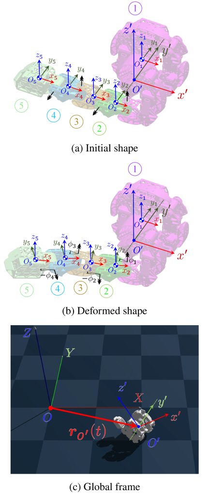
Fig. 2. Definition of coordinate systems 30. (a) Initial shape of the robot. The joint frame is defined for each joint. (b) Deformed shape of the robot. The joint frame changes according to the deformation of the robot. (c) Global frame. The world coordinate system is fixed to the ground, and the body coordinate system is fixed to the body link of the robot and changes according to the motion of the body.
| Calculation conditions: | ||
| Solver | Implicit fast | |
| Time step | \(\Delta t\) | \(2.0 \times 10^{-3} \: \mathrm{s}\) |
| Control period | \(\Delta T\) | \(50.0 \times 10^{-3} \: \mathrm{s}\) |
| Precision | FP32 | |
| Position gain | \(k_\mathrm{p}\) | 100 Nm/rad |
| Velocity gain | \(k_\mathrm{v}\) | 1.0 Nms/rad |
| Joint damping | 2.0 Nms/rad |
3. Reinforcement Learning Framework for Rolling Locomotion
We formulate the target reaching task in the rolling locomotion of a snake-like robot as a Markov decision process (MDP) in which an agent learns the optimal action through interaction with the environment. An MDP is defined as a tuple \(\mathcal{M} = \left( \mathcal{S}, \mathcal{A}, \mathcal{T}, r, \gamma \right)\), where the state space \(\mathcal{S}\) is a set of observations such as joint angles and angular velocities of the robot and the relative orientation vector of the target as seen from the body coordinate system, and the action space \(\mathcal{A}\) is a set of continuous actions that determine the target angular velocity of each joint. The transition probability \(\mathcal{T}\) represents the probability distribution \(P(s' | s, a)\) of transitioning to the next state \(s' \in \mathcal{S}\) when taking action \(a \in \mathcal{A}\) in the current state \(s \in \mathcal{S}\), and the physics simulator Genesis is responsible for its dynamics in this study. The reward function \(r\) defines the immediate reward \(r = R(s, a)\) obtained from the environment when selecting action \(a\) in state \(s\), and the discount factor \(\gamma \in [0, 1)\) is a coefficient that converts future rewards into present value. The goal of the agent is to acquire an optimal policy \(\pi(a|s)\) that maximizes the expected cumulative discounted reward \(E [\sum_{t=0}^{\infty} \gamma^t r_t]\) through a series of trials. The rolling locomotion by center of gravity shift targeted in this study involves a physical delay before the driving of the actuators manifests as the actual body behavior. Therefore, this system needs to be treated as a delayed Markov decision process35. The details of the treatment will be described in the explanation of the state space.
3.1. Action Space
The action is defined as in the previous research 28,30. The angle range and angular velocity of the actuators have physical limitations. To satisfy the driving angle range constraint \(\phi_{\mathrm{min},l} \leq \phi_{\mathrm{d},l}(t) \leq \phi_{\mathrm{max},l}\) and the angular velocity constraint \(\left| \mathrm{d} _t \phi_{\mathrm{d},l}(t)\right| \leq \omega_\mathrm{max}, \: l \in \{1,\ldots, N_\mathrm{body}-1\}\), the following action expressions are introduced,
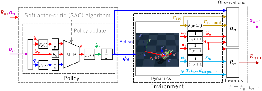
Fig. 3. Overview of the reinforcement learning framework for rolling locomotion. The agent receives the observation \(\boldsymbol{o}(t)\) from the environment and outputs the action \(\boldsymbol{a}(t)\) to the environment at each control step. The action is converted to the target joint angle \(\boldsymbol{\phi}_\mathrm{d}(t)\) by Eqs. (1)–(3), and the robot moves according to the target joint angle. The reward is calculated based on the state of the robot and the target location, and the agent learns to maximize the expected value of the discounted reward.
| Angular velocity constraints | \(\omega_\mathrm{max}\) | \(\dfrac{\pi}{2} \: \mathrm{rad/s}\) |
| Angle constraints | \(\phi_{\mathrm{min},1}\) | \(-\dfrac{\pi}{12} \: \mathrm{rad}\) |
| \(\phi_{\mathrm{min},2}\) | \(-\dfrac{\pi}{2} \: \mathrm{rad}\) | |
| \(\phi_{\mathrm{min},3}\) | \(-\dfrac{\pi}{3} \: \mathrm{rad}\) | |
| \(\phi_{\mathrm{min},4}\) | \(-\dfrac{\pi}{2} \: \mathrm{rad}\) | |
| \(\phi_{\mathrm{max},k}\) | \(\dfrac{\pi}{2} \: \mathrm{rad}\) |
3.2. State Space
The body link of the snake-like robot are equipped with an accelerometer and a gyroscope (BNO055, Bosch Sensortec GmbH, Germany). The orientation of the gravity acceleration measured by the accelerometer can be used to determine the rotation angle, and the value of the angular velocity measured by the gyroscope can be used to evaluate the moving direction. Therefore, the gravity and angular velocity are included in the state space. The time integration of the target joint angle \(\boldsymbol{\phi}_\mathrm{d}\) shown in Eq. (2) may cause drift. To avoid this, the target joint angle shown in Eq. (1) is also included in the observed values as input to the MLP (Fig. 3). Since the observed gravity acceleration \(\boldsymbol{a}_\mathrm{o}(t)\) and angular velocity \(\boldsymbol{\omega}_\mathrm{o}(t)\) contain noise, the values \(\tilde{\boldsymbol{a}}_\mathrm{o}(t)\) and \(\tilde{\boldsymbol{\omega}}_\mathrm{o}(t)\) obtained by passing through a first-order lag low-pass filter are used as observed values. Here, the time constant of the low-pass filter is \(\Delta T/T_a = 0.2, \ \Delta T/T_\omega = 0.2\). This system is a system in which the action \(\boldsymbol{a}\) corresponds to the target angular velocity \(\dot{\boldsymbol{\phi}}_\mathrm{d}\) of the actuator, and the rolling locomotion is generated by the center of gravity shift due to the deformation of the movable link and the reaction force from the floor. Therefore, it becomes a system in which the change of the action acts with a time delay, and it is necessary to treat it as a Markov decision process with a time delay 35. Therefore, in order to improve the convergence of the reinforcement learning of this system, we introduce a buffered observation 36. In this system, the action \(\boldsymbol{a}\) corresponds to the target angular velocity \(\dot{\boldsymbol {\phi}}_\mathrm{d}\) of the actuator, and the rolling locomotion is generated by the center of gravity shift due to the deformation of the movable link and the reaction force from the floor. Since the rolling lags behind the movement of the links, these observations are buffered and treated as time-series information 36.
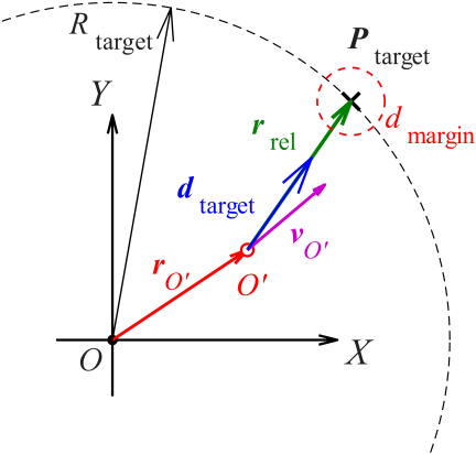
Fig. 4. Geometric definitions of the target-following task. The target \(P_{\text{target}}\) is placed on a circle of radius \(R_{\text{target}}\). The relative vector \({\boldsymbol{r}}_{\text{rel}}\) and the target direction unit vector \({\boldsymbol{d}}_{\text{target}}\) are defined based on the current position \({\boldsymbol{r}}_{O'}\) of the body link center \(O'\). \({\boldsymbol{v}}_{O'}\) represents the current velocity vector of the body link.
The above observations are the same as those used in previous studies for rolling straight 28,30. Since the purpose of this study is to design a controller capable of not only linear motion but also turning motion, the information indicating the target reaching direction is added to the state space. The overview of the added observations is shown in Fig. 4. The target location \(P_{\mathrm{target}}\) is randomly placed on the circumference of the fixed radius \(R_{\mathrm{target}}\). Since the center of gravity changes continuously due to the movement of the links, the geometric center \(O'\) of the body link is adopted as the physical reference point in the simulation instead of the center of gravity of the robot. The relative vector between the target location and the center of the body link \(O'\) is defined as \(\boldsymbol{r}_{\mathrm{rel}} := P_{\mathrm{target}} - \boldsymbol{r}_{O'}\), and the value obtained by normalizing this relative vector \(\boldsymbol{r}_{\mathrm{rel}}\) by the radius \(R_{\mathrm{target}}\) is added to the state space. To learn the spatial positional relationship, this relative vector \(\boldsymbol{r}_{\mathrm{rel}}\) is transformed into the body coordinate system \(\boldsymbol{r}_{\mathrm{rel,local}}\) using the inverse rotation of the quaternion \(\boldsymbol{q}\) representing the current pose of the robot. The resulting vector, normalized by the radius \(R_{\mathrm{target}}\), is used as the relative bearing vector \(\boldsymbol{o}_5(t_{n})\). This allows the agent to directly observe the relative bearing of the target with respect to its own direction of travel (\(x'\)-axis) rather than the absolute position in the world coordinate system.
Finally, the observations are defined as follows:
3.3. Reward Function
The total reward \(R_n\) at each step is defined as the sum of the step reward \(r_{\mathrm{step},n}\) defined by the product of multiple performance indices, the potential reward \(r_{\mathrm{pot},n}\) based on the change in distance to the target location, and the time penalty \(\rho_{\mathrm{time},n}\) as follows:
3.3.1. Rolling Velocity Reward
The rolling velocity reward is an index for evaluating the forward performance of the robot’s rolling locomotion. It is defined as follows using the angular velocity around the pitch axis in the body coordinate system obtained from the gyro attached to the torso link, \(\tilde{\omega}_{\mathrm{o},2}\), and the radius \(R_{\mathrm{body}}\) when the robot deforms into a tire shape.
3.3.2. Directionality Reward
The directionality reward is an index for evaluating how accurately the robot’s direction of travel is oriented towards the target location. As shown in Fig. 4, it is defined using the cosine similarity of the velocity vector of the body link in the world coordinate system, \(\boldsymbol{v}_{\mathrm{o'}}\), and the unit vector in the direction from the current position to the target location, \(\boldsymbol{d}_{\mathrm{target}}\), as follows:
3.3.3. Stability Reward
The stability reward is an index for evaluating the stability of the motion and the maintenance of the ideal tire shape during movement. This index is defined as a weighted average using a weight vector \(\boldsymbol{w} = [0.5 \ 1.0 \ 1.0 \ 1.0]^\mathrm T\) for the following four evaluation indices \(p_{n,i}\):
3.3.4. Left Turn Correction
The robot used in this study needs to move the links laterally with respect to the rotation direction when shifting the center of gravity, and it tends to be physically more difficult to turn left than right when rotating in the forward direction. To compensate for this physical bias and encourage learning smooth guidance in all directions, a correction factor is introduced that amplifies the reward only when the target is located on the left side of the robot and the robot is facing the target direction. Let \(\theta_{\mathrm{azimuth}}\) be the azimuth angle of the target location as seen from the robot, then it is defined as follows:
3.3.5. Potential Reward
To encourage steady approach to the target location and to mitigate reward sparsity, a potential reward \(r_{\mathrm{pot},n}\) based on the change in distance to the target location is introduced. Let \(d(t_n)\) be the distance between the robot’s body link and the target location at time \(t_n\), then it is defined as follows:
3.3.6. Goal Achievement Reward and Time Penalty
When the distance \(d_n\) from the center of the body link to the target location in the world coordinate system reaches a certain tolerance \(d_{\mathrm{margin}}\), it is judged that the target has been reached. The value of \(d_{\mathrm{margin}}\) is set to 0.3 m, which is based on the width of the robot’s body in the turning mode (the horizontal width in the top view of Fig. 1(c)) and indicates the range within which it can be considered that the robot has sufficiently reached the target location. At the point when the achievement is judged, the episode ends and the following goal achievement reward is given as a success reward for the episode.
The coefficients in Eq. (18) are determined by a logical design philosophy based on the stepwise promotion of learning and the motion characteristics of previous studies. The constant term in the first term is an incentive for achieving the goal itself in the early stages of learning, and there is a trade-off in that if this is too small, it may fall into a local solution where it does not reach the target and earns step rewards along the way, while if it is too large, the discontinuous large reward can destabilize the estimation of the value function and cause learning to collapse. The coefficient related to the remaining time in the second term is designed to encourage more rapid dynamic path selection after achieving the minimum arrival. This coefficient is determined based on the performance in the straight-line simulation in a previous study 28, which took about 7 seconds to move 3 m, and the estimate that it would be possible to reach in about 7 seconds in this task involving turning if an ideal path is selected. With a maximum episode length of 30 seconds, if it reaches in the fastest time (7 seconds), the remaining time would be 23 seconds, and by setting the coefficient to 2, it provides a balance such that the additional bonus does not become excessively dominant compared to the constant reward, while still providing a sufficient slope to optimize rapidity.
On the other hand, to suppress unnecessary stagnation, a uniform time penalty of \(\rho_{\mathrm{time}} = 0.05\) is imposed on each step until reaching the target. Also, if the robot is judged to have fallen (when the acceleration other than the pitch axis exceeds a threshold), a negative reward is given and the episode is forced to end.
3.4. Policy Structure
The policy of the agent is constructed using a MLP. The structure of the network inherits the configuration of a previous study that has an effective observation buffer for systems with time delays. Both the policy network and the value function network consist of fully connected networks with 2 hidden layers of 256 units each. The input observation vector \(\boldsymbol{o}(t_n)\) and the output action \(\boldsymbol{a}(t_n)\) are defined as follows:
4. Controller Design by Reinforcement Learning
4.1. Simulation Setup
To train and evaluate the proposed reinforcement learning algorithm, the physics simulation environment Genesis (v0.2.1) was adopted. Genesis is a physics engine that enables fast computation of multibody dynamics and can simulate the motion model of the snake-like robot described in Section 2. Within the simulator, the interaction between the robot and the floor is calculated based on rigid body dynamics. Considering the stability of the calculations, the time step for physics calculations was set to \(\Delta t = 2.0 \times 10^{-3}\,\mathrm{s}\). On the other hand, the control cycle for policy updates and action decisions by the agent was set to \(\Delta T = 50.0 \times 10^{-3}\,\mathrm{s}\) (\(20\,\mathrm{Hz}\)), which is designed to account for the response characteristics of the actual actuators and the computational load on a SBC. The maximum episode time was set to \(T_{\max} = 30.0\,\mathrm{s}\). However, to improve learning efficiency, if the robot is judged to have fallen, a negative reward is given and the episode is set to end early. The robot is defined as having fallen when the value obtained by passing the acceleration in the \(y'\)-axis (longitudinal direction of the robot) in the body coordinate system through a low-pass filter exceeds 80% of the gravitational acceleration \(g\).
Regarding the observation buffer size used for constructing the state space, \(N_d = 20, N_{\mathrm{skip}} = 2\) was set. The targeted rolling locomotion of the snake-like robot involves a time lag from the driving of the joints to the actual rolling behavior of the robot, so using only the latest observation (\(N_d = 1\)) makes it difficult to learn the causal relationship and degrades movement performance 28,29,30. In particular, when the buffer size \(N_d\) is small, the lack of past information to compensate for the time delay causes large oscillations in the joint angles and reduces the rolling speed. On the other hand, expanding the buffer size allows for more accurate learning of causal relationships with time delays, and it has been quantitatively demonstrated in previous research 30 that this results in increased cumulative rewards through the generation of smooth movements.
The physical parameters and contact dynamics model used for the analysis are based on the estimation results in a previous study 30 that conducted rolling locomotion experiments using a snake-like robot referenced in this research. Specifically, the friction coefficient \(\mu = 0.10\) and contact resolution time \(\tau_c = 0.01\) s in the contact model were obtained by fitting the time series data of the rotation angle obtained from a free rotation experiment where the snake-like robot was manually rolled on a smooth and flat floor surface with the behavior of the simulation. The reason for narrowing down the environmental characteristics to this single condition is to fix the physical environment that can be physically reproduced and executed as a basis for future verification experiments using the robot. By fixing the environment based on an established experimental setup, the main scope of this paper is to verify the effectiveness of the proposed omnidirectional guidance strategy. While it is difficult to perfectly model the physical contact phenomena and friction characteristics with the ground in the simulation, these identified parameters provide an equivalent contact model that can reproduce the rolling locomotion, and the reproducibility has been experimentally demonstrated in the previous study 30.
4.2. Hyperparameters and Training Settings
The soft actor-critic (SAC) algorithm, an off-policy DRL algorithm, is used for policy learning 37,38,39. SAC has the characteristic of maximizing the policy’s entropy in addition to maximizing the expected reward, which leads to high exploration efficiency and less susceptibility to local optima. The learning is performed using stable baseline3 (SB3, v2.4.0), and the specific hyperparameters are shown in Table 5 40. The learning rate for both the policy network and the value function network is set to \(3 \times 10^{-4}\), and the size of the replay buffer for storing past experiences is set to \(1.0 \times 10^{6}\). The discount factor for rewards is set to \(\gamma = 0.99\), and a batch of 256 samples is extracted for learning at each update step. By introducing an automatic temperature adjustment parameter for entropy adjustment, it maintains appropriate exploration according to the progress of learning. These parameter values are based on those used in a previous study on the SAC algorithm 39. The training continues until the total reward converges and the success rate of reaching the target location stabilizes sufficiently.
| Parameter | Value |
| Learning rate | \(3.0 \times 10^{-4}\) |
| Replay buffer size | \(1.0 \times 10^{6}\) |
| Entropy regularization coefficient | Auto |
| Batch size | 256 |
| Discount factor (\(\gamma\)) | 0.99 |
| Gradient steps per update | 1 |
4.3. Initialization
At the beginning of each episode, the \(x'\)-, \(y'\)-coordinates of the center of the robot’s body link \(O'\) are initialized to coincide with the origin \((X, Y) = (0, 0)\) of the world coordinate system. As a reference for the initial orientation, the longitudinal direction of the robot is set to the positive \(X\)-axis direction of the world coordinate system, but the following initial conditions are set to enhance the robustness of learning. The pitch angle of the body is given a random variation based on a uniform distribution in the range of \(\pm 30°\) (\(\pm \pi/6\) rad). This allows the operation to start from different body inclinations for each episode.
5. Results and Discussion
5.1. Learning Performance and Convergence
To evaluate the effectiveness of the proposed target-following control method, reinforcement learning was conducted on the physics simulator Genesis. To assess the convergence and stability of learning, five independent learning trials were conducted using different random seeds, and the transition of cumulative rewards is shown in Fig. 5. The solid line in the figure represents the average of the five trials, and the shaded area represents the standard deviation. Examining the learning curves, it can be confirmed that in all trials, the reward stabilizes at a high value (around 270 or above) around \(4.0 \times 10^6\) steps, indicating convergence. Although the target is randomly placed in all directions (azimuth angle \(\theta_{\mathrm{target}} \in [-\pi, \pi)\)) from the early stages of learning, the reward increases smoothly without stagnation, demonstrating that the proposed method has high learning efficiency even for the complex task of omnidirectional target following. This is considered to be because the unit vector of the target direction (from \(\boldsymbol{o}_4\) to \(\boldsymbol{o}_5\)) introduced in the state space can directly and efficiently present the relative directional information of the target location with respect to the agent’s heading direction. Furthermore, the extremely small variance between trials in the later stages of learning indicates that the proposed reward design and network structure have robust learning performance that is not dependent on the initial values.
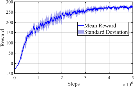
Fig. 5. Reward curve of the SAC agent.
To evaluate the validity of the convergence value of the total reward around 270, based on the environment specification that the episode ends immediately upon reaching the target, we estimate the theoretical maximum potential of the reward when reaching the target location at the highest speed. As shown later in Fig. 9 (in Section 5.4), the actual arrival time with the acquired policy is about 7 s (equivalent to 350 steps with a control cycle of \(\Delta t = 0.02\,\mathrm{s}\)), at which point the environment resets. With a maximum episode length of 30 s, the remaining time at the point of arrival would be 23 s, resulting in a goal achievement bonus of \(66.0\) and a cumulative time penalty of \(-17.5\) according to Eq. (18). Also, the cumulative potential reward \(r_{\mathrm{pot}}\) when reaching the target location from an initial distance of 3.0 m is calculated as \(50 \times (3.0 - 0) = 150.0\) under the weight coefficient \(w_{\mathrm{pot}} = 50\), as the intermediate term mathematically cancels out. Including the scaling factor \(\alpha = 2\) and considering a good cruising orientation error (\(J_{\mathrm{dir}} = [0.8 \ 1.0]\)) based on the cumulative performance of 20 s in a previous study, which is time-converted to 7 s for this task involving turning, the maximum upper limit estimate of the cumulative step reward \(r_{\mathrm{step}}\) is \(132.3\) (\(49.0 \times 0.9 \times 3.0\)) considering the dynamic characteristics that \(J_{\mathrm{dir}} = 1.0\) cannot be simultaneously satisfied and is limited to about 0.9 in the turning phase where the left turn correction coefficient \(\beta_{\mathrm{left}} = 3.0\) functions due to geometric constraints. Thus, the overall theoretical upper limit range is derived to be approximately 237.7 to 330.8. The fact that the actual learning curve converges around 270, which is a reasonable score range within the upper limit range (247.5 for pure straight cruising), indicates that the acquired control policy has highly learned and utilized the difficult left turn incentive, and has achieved a good balance between rapidity and orientation accuracy in approaching the target location.
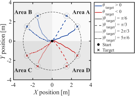
Fig. 6. Trajectories of the body link for five independent learning trials. The target location is indicated by a red star, and the trajectories are shown in different colors for each trial.
5.2. Analysis of Body Link Trajectories
In this section, to evaluate the characteristics of the paths selected by the trained agent for targets in all directions, the trajectories of the body link are analyzed. Fig. 6 shows the body link trajectories when the target is placed at eight target angles (\(\pm \pi/6, \pm \pi/3, \pm 2\pi/3, \pm 5\pi/6\) rad) covering all quadrants centered on the initial position. First, in the forward area where the target exists in the forward direction of the robot (Area A: \(+\pi/6, +\pi/3\) rad and Area D: \(-\pi/6, -\pi/3\) rad), the robot smoothly transitions from the initial forward state to a turning motion, reaching the target location by drawing an arc close to the shortest distance. As the target angle moves away from \(0°\) (approaching the true side), it is confirmed that the turning radius is appropriately adjusted and converges to the target without overshooting.
On the other hand, when the target is placed in the rear area (Area B: \(-2\pi/3, -5\pi/6\) rad and Area C: \(+2\pi/3, +5\pi/6\) rad), the agent selects a characteristic path. In these cases, instead of performing a forward roll and making a large turn, the agent skillfully manipulates the center of gravity shift and the reaction force from the floor to directly orient towards the target direction by rolling backward. Even when the target position changes from the front to the rear, the smoothness of the trajectory is maintained, demonstrating that the proposed method can learn a seamless movement space for all directions without forcing the agent to be aware of discontinuous state changes such as forward or backward. Comparing the trajectories for all eight directions, a high degree of symmetry in the left and right directions can be observed, and there is no bias towards a specific turning direction. This indicates that the policy has overcome the physical characteristic of the robot that tends to turn towards the right direction.
5.3. Motion Analysis Using Snapshots
To clarify the specific control strategies acquired by the trained agent, the behavior of the robot is analyzed using snapshots during the simulation. The turning motion is examined to understand how it is achieved.
5.3.1. Area A (Forward Rolling and Left Turn)
Figure 7 shows a series of snapshots of the turning motion in Area A. This area is a turning phase centered on forward movement, where the robot attempts to turn left while extending the movable link on the right side of the body. By confirming the initial states at \(t=0.30\) s and \(0.63\) s just after the start of the motion, it can be observed that the robot generates turning torque by using specific links as support and achieves rapid heading changes towards the target direction. This tendency can also be confirmed in Fig. 6, where the trajectory extends from the origin towards the target direction even though the robot is initially placed parallel to the \(x\)-axis.
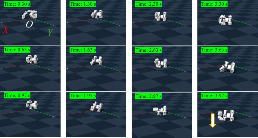
Fig. 7. Snapshots of the rolling locomotion in Area A.
Due to the physical structure of the robot, when the links are extended significantly in the direction of movement for center of gravity shift, a force that deflects towards the right direction naturally acts due to inertia and mass bias. However, in the snapshots at \(t=1.97\) and \(3.97\) s, it was observed that the timing of the leading link contacting the ground is precisely controlled. This control can also be confirmed in Fig. 6, where the trajectory changes sharply towards the target direction at the timing of contact. By converting the ground reaction force obtained at the moment of this contact into a propulsive force towards the left direction, it is considered that the right deflection due to the physical structure is canceled out, allowing for dynamic trajectory correction.
5.3.2. Area C (Backward Rolling and Left Turn)
Next, the analysis results of the left turn motion with backward rolling, which is Area C, are shown in Fig. 8. In this area as well, it can be confirmed that the robot performs heading changes towards the target direction at a very early stage immediately after the start of the motion, achieving rapid direction changes through interaction with the environment. Notably, compared to the snapshots in Area A, it can be observed that even at the same time, the robot has moved to a position closer to the target from the initial position. This is considered to be because Area C is a phase where the robot turns towards the left side where the movable link exists, allowing for more direct and efficient utilization of the mass inertia of the link as a turning moment. Unlike in Area A, the absence of the need for directional adjustment when the movable link contacts the ground is also considered to be one of the factors that enables more efficient turning. In fact, the trajectory in Area C is smoother compared to the trajectory in Area A, and there is no sudden change in direction. Instead, by extending the movable link in the lateral direction, the center of gravity shifts significantly, allowing for heading changes towards the target direction.
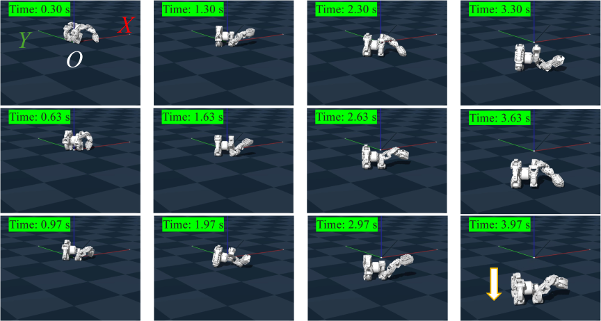
Fig. 8. Snapshots of the rolling locomotion in Area C.
5.4. Time-Series Analysis of Joint Angles
The time-series of joint angles \(\phi_{i}\) (\(i=1, \dots, 4\)) during the turning motion for target locations in all eight directions are analyzed to evaluate how the policy manipulates the center of gravity to achieve guidance. Fig. 9 shows the responses of each joint at the time of reaching the target, particularly for the four directions that require significant turning (\(\pm \pi/3, \pm 2\pi/3\) rad) in each area (Areas A–D). Since it is expected that the motion differs for forward or backward rolling and for left or right turns in each quadrant, these four directions were selected for analysis. A characteristic observation is that the time to reach the target in Area D is slower than in the other areas. While it may seem faster to turn right while rolling forward to reach Area D, the robot performs a motion where it rotates more than 90° around the \(Z\)-axis in place in a leftward direction before rolling backward. This motion causes the time to reach the target to be longer.
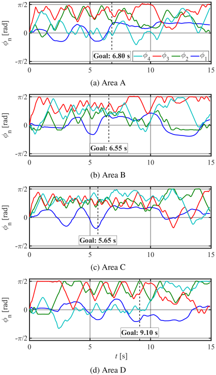
Fig. 9. Time-series of joint relative angles for target locations in Areas A–D.
A common aspect of all motions is that at the start of the motion, the third joint moves with a larger amplitude compared to the other joints. At this time, the robot is performing a direction change near the origin, and as shown in the first snapshot in Figs. 7 and 8, it is supporting itself by contacting the tip of the movable link with the ground. Also, focusing on the time-series of the third joint, it takes time for Areas B and D to enter a periodic state. Since the movable link is good at performing direction changes by receiving a reaction force that kicks the ground in the opposite direction of the robot, it is considered that it is easier to transition from the initial position to the targets in Areas A and C.
Next, comparing the results of Areas A and B, while the previous study only verified forward rolling, in Area B, the target is reached by rolling backward. Although the time to reach the target is almost the same, there is a significant difference in the time-series of joint angles between Area A and Area B. In Area A, the second joint moves significantly, while in Area B, the fourth joint moves significantly. However, this difference in joint movement is not considered to be due to the difference between forward and backward rolling, but rather simply due to the difference in target position. Area D reaches the target by rolling backward, but the waveforms of the joints are similar to Area A. From this, it is considered that the difference between forward and backward rolling is not directly related to the difference in joint movements. Rather, the fact that Area A, which is rolling forward, and Area D, which is rolling backward, have similar time-series of joint angles shows that the same joint movements can lead to reaching the target even with forward or backward rolling.
Finally, regarding the behavior after reaching the target, since the episode ends simultaneously with reaching the target during learning, the behavior after reaching the target is outside the scope of learning. However, it can be confirmed that the joint angles continue to change even after reaching the target. This is because there is no guarantee that the tip of the link is positioned directly under the robot at the time of reaching the target, and rather, it is often the case that the tip of the link is positioned in front or behind the target even after reaching it. Therefore, if the link is suddenly stopped, the robot rotates in a direction away from the target location. To suppress that rotation, it can be confirmed that the link continues to change its joint angles without stopping even after reaching the target location.
6. Conclusions
In this study, we proposed an omnidirectional target-following control method for snake-like robots based on center of gravity shift and ground reaction forces, using DRL, and verified its effectiveness. The main findings obtained from this study are as follows.
-
・
Realization of Omnidirectional Following Control: By introducing the relative azimuth vector of the target with respect to the body coordinate system into the observation space, it was shown that the agent can utilize the directional information to learn the following control even for targets placed in all directions.
-
・
Evaluation of Convergence and Stability: In five independent learning trials, the reward stabilized at high values in all trials, confirming that the proposed method has robust, high learning performance for the omnidirectional target-following task.
-
・
Compensation for Physical Bias: The policy acquired through learning automatically compensates for the rightward deflection characteristic due to the robot’s structure, achieving symmetric turning performance that is independent of the target azimuth.
-
・
Trajectory Correction through Timing of Ground Contact: As a result of motion analysis, it was observed that the agent precisely controls the timing of specific links contacting the ground, converting the ground reaction force at the moment of contact into propulsive force for turning.
These findings represent an important step towards realizing omnidirectional target-following control for snake-like robots using center of gravity shift and ground reaction forces, and future research is expected to further develop this by applying it to real machines and evaluating performance in more complex environments. In particular, to further enhance the robustness against uncertain environments by absorbing and overcoming the simulation-to-reality modeling errors that arise in unknown surface properties, the introduction of domain randomization that diversifies physical parameters such as friction coefficients and joint torque limits during learning is an important future task.
Acknowledgments
This study was supported by the Mazda Foundation, Japan, JSPS Grant-in-Aid for Scientific Research (C), Japan, No. 25K07667 and JST SPRING, Japan, No. JPMJSP2139.
- [1] X. Zang, Y. Liu, Z. Lin, C. Zhang, and S. Iqbal, “Two multi-linked rescue robots: Design, construction and field tests,” J. of Advanced Mechanical Design, Systems, and Manufacturing, Vol.10, No.6, Article No.JAMDSM0089, 2016. https://doi.org/10.1299/jamdsm.2016jamdsm0089
- [2] T. Kamegawa, T. Akiyama, S. Sakai, K. Fujii, K. Une, Y. Wang, Y. Matsumura, T. Kishutani, E. Nose, Y. Yoshizaki, and A. Gofuku, “Development of a separable search-and-rescue robot composed of a mobile robot and a snake robot,” Advanced Robotics, Vol.34, No.2, pp. 132-139, 2020. https://doi.org/10.1080/01691864.2019.1691941
- [3] F. Enner, D. Rollinson, and H. Choset, “Motion estimation of snake robots in straight pipes,” 2013 IEEE Int. Conf. on Robotics and Automation, pp. 5168-5173, 2013. https://doi.org/10.1109/ICRA.2013.6631316
- [4] I. N. Ismail, A. Anuar, K. S. M. Sahari, M. Z. Baharuddin, M. Fairuz, A. Jalal, and J. M. Saad, “Development of in-pipe inspection robot: A review,” 2012 IEEE Conf. on Sustainable Utilization and Development in Engineering and Technology (STUDENT), pp. 310-315, 2012. https://doi.org/10.1109/STUDENT.2012.6408425
- [5] N. Matsumoto, M. Tanaka, M. Nakajima, M. Fujita, and K. Tadakuma, “Development of a folding arm on an articulated mobile robot for plant disaster prevention,” Advanced Robotics, Vol.34, No.2, pp. 89-103, 2020. https://doi.org/10.1080/01691864.2019.1689167
- [6] X. Hou, Y. Shi, L. Li, Y. Tian, Y. Su, T. Ding, and Z. Deng, “Revealing the Mechanical Characteristics via Kinematic Wave Model for Snake-Like Robot Executing Exploration of Lunar Craters,” IEEE Access, Vol.8, pp. 38368-38379, 2020. https://doi.org/10.1109/ACCESS.2020.2971221
- [7] T. S. Vaquero, G. Daddi, R. Thakker et al., “EELS: Autonomous snake-like robot with task and motion planning capabilities for ice world exploration,” Science Robotics, Vol.9, No.88, Article No.eadh8332, 2024. https://doi.org/10.1126/scirobotics.adh8332
- [8] M. Tesch, K. Lipkin, I. Brown, R. Hatton, A. Peck, J. Rembisz, and H. Choset, “Parameterized and Scripted Gaits for Modular Snake Robots,” Advanced Robotics, Vol.23, No.9, pp. 1131-1158, 2009. https://doi.org/10.1163/156855309X452566
- [9] T. Takemori, M. Tanaka, and F. Matsuno, “Hoop-Passing Motion for a Snake Robot to Realize Motion Transition Across Different Environments,” IEEE Trans. on Robotics, Vol.37, No.5, pp. 1696-1711, 2021. https://doi.org/10.1109/TRO.2021.3063438
- [10] T. Takemori, M. Tanaka, and F. Matsuno, “Gait design of a snake robot by connecting simple shapes,” 2016 IEEE Int. Symposium on Safety, Security, and Rescue Robotics (SSRR), pp. 189-194, 2016. https://doi.org/10.1109/SSRR.2016.7784297
- [11] M. Tesch, J. Schneider, and H. Choset, “Expensive multiobjective optimization for robotics,” 2013 IEEE Int. Conf. on Robotics and Automation, pp. 973-980, 2013. https://doi.org/10.1109/ICRA.2013.6630691
- [12] S. Hasanzadeh and A. A. Tootoonchi, “Ground adaptive and optimized locomotion of snake robot moving with a novel gait,” Autonomous Robots, Vol.28, pp. 457-470, 2010. https://doi.org/10.1007/s10514-010-9179-y
- [13] A. Crespi and A. J. Ijspeert, “Online Optimization of Swimming and Crawling in an Amphibious Snake Robot,” IEEE Trans. on Robotics, Vol.24, No.1, pp. 75-87, 2008. https://doi.org/10.1109/TRO.2008.915426
- [14] S. Jiang, A. Salagame, A. Ramezani, and L. L. S. Wong, “Snake Robot with Tactile Perception Navigates on Large-scale Challenging Terrain,” 2024 IEEE Int. Conf. on Robotics and Automation (ICRA), pp. 5090-5096, 2024. https://doi.org/10.1109/ICRA57147.2024.10611384
- [15] S. Jiang, A. Salagame, A. Ramezani, and L. L. Wong, “Hierarchical RL-Guided Large-scale Navigation of a Snake Robot,” 2024 IEEE Int. Conf. on Advanced Intelligent Mechatronics (AIM), pp. 1347-1352, 2024. https://doi.org/10.1109/AIM55361.2024.10637006
- [16] J. Naish, J. Rodriguez, J. Zhang, B. Jones, G. Daddi, A. Orekhov, R. Royce, M. Paton, H. Choset, M. Ono, and R. Thakker, “Reinforcement learning-driven parametric curve fitting for snake robot gait design,” Proc. of the 6th Annual Learning for Dynamics & Control Conf., pp. 1715-1727, 2024.
- [17] H. Kurokawa, A. Kamimura, E. Yoshida, K. Tomita, S. Murata, and S. Kokaji, “Self-reconfigurable modular robot (M-TRAN) and its motion design,” 7th Int. Conf. on Control, Automation, Robotics and Vision (ICARCV 2002) pp. 51-56, 2002. https://doi.org/10.1109/ICARCV.2002.1234789
- [18] J. Zhao, X. Cui, Y. Zhu, and S. Tang, “A new self-reconfigurable modular robotic system UBot: Multi-mode locomotion and self-reconfiguration,” 2011 IEEE Int. Conf. on Robotics and Automation, pp. 1020-1025, 2011. https://doi.org/10.1109/ICRA.2011.5980293
- [19] X. Wang, H. Jin, Y. Zhu, B. Chen, D. Bie, Y. Zhang, and J. Zhao, “Serpenoid polygonal rolling for chain-type modular robots: A study of modeling, pattern switching and application,” Robotics and Computer-Integrated Manufacturing, Vol.39, pp. 56-67, 2016. https://doi.org/10.1016/j.rcim.2015.12.003
- [20] A. Salagame, N. Bhattachan, A. Caetano et al., “How Strong a Kick Should be to Topple Northeastern’s Tumbling Robot?,” 2024 IEEE Int. Conf. on Advanced Intelligent Mechatronics (AIM), pp. 76-81, 2024. https://doi.org/10.1109/AIM55361.2024.10637166
- [21] A. Salagame, H. Noyes, E. Sihite, A. Kalantari, and A. Ramezani, “Crater Observing Bioinspired Rolling Articulator (COBRA),” Advanced Intelligent Systems, Vol.8, No.3, Article No.2500352, 2026. https://doi.org/10.1002/aisy.202500352
- [22] K. Miki, C. W. Chin, and M. Tanaka, “Snake Robot with Opposing Helix Gait for Transporting Cylindrical Objects,” IEEE Robotics and Automation Letters, Vol.11, No.2, pp. 2098-2105, 2026. https://doi.org/10.1109/LRA.2025.3645515
- [23] A. Yamano, Y. Ikeda, K. Imai, and M. Chiba, “Efficient rolling motion for snake-like robots utilizing center of gravity shift,” Mechatronics, Vol.94, Article No.103024, 2023. https://doi.org/10.1016/j.mechatronics.2023.103024
- [24] Y. Sugiyama and S. Hirai, “Crawling and Jumping by a Deformable Robot,” The Int. J. of Robotics Research, Vol.25, Nos.5-6, pp. 603-620, 2006. https://doi.org/10.1177/0278364906065386
- [25] Y. Wang, C. Wu, L. Yu, and Y. Mei, “Trajectory planning of a rolling robot of closed five-bow-shaped-bar linkage,” Robotics and Computer-Integrated Manufacturing, Vol.53, pp. 81-92, 2018. https://doi.org/10.1016/j.rcim.2018.03.004
- [26] Y. Wang, C. Wu, L. Yu, and Y. Mei, “Dynamics of a rolling robot of closed five-arc-shaped-bar linkage,” Mechanism and Machine Theory, Vol.121, pp. 75-91, 2018. https://doi.org/10.1016/j.mechmachtheory.2017.10.010
- [27] A. Yamano, T. Kimoto, and M. Chiba, “Design of Rolling Motion for Snake-like Robots using Center-of-Gravity Shift,” J. of Mechanisms and Robotics, Vol.17, No.6, Article No.061011, 2025. https://doi.org/10.1115/1.4067307
- [28] T. Kimoto, S. Suzuki, A. Yamano, and T. Iwasa, “Rolling Motion Control in a Snake Robot Using Center-of-Mass Shift and Reinforcement Learning-Based Motion Exploration,” 2025 JSME Conf. on Robotics and Mechatronics, Vol.2025, Article No.2P1-P11, 2025 (in Japanese). https://doi.org/10.1299/jsmermd.2025.2P1-P11
- [29] S. Suzuki, A. Yamano, T. Kimoto, and T. Iwasa, “Study on the Rolling Motion of a Snake-Like Robot That Transforms into a Parallel Two-Wheeled Vehicle Using Deep Reinforcement Learning,” 2025 25th Int. Conf. on Control, Automation and Systems (ICCAS), pp. 1485-1490, 2025. https://doi.org/10.23919/ICCAS66577.2025.11301120
- [30] A. Yamano, S. Suzuki, T. Kimoto, and T. Iwasa, “Deep reinforcement learning-based design with observation buffer of rolling motion for snake-like robots,” Robotics and Autonomous Systems, Vol.199, Article No.105370, 2026. https://doi.org/https://doi.org/10.1016/j.robot.2026.105370
- [31] H. C. Astley, C. Gong, J. Dai, M. Travers, M. M. Serrano, P. A. Vela, H. Choset, J. Mendelson III, D. Hu, and D. Goldman, “Modulation of orthogonal body waves enables high maneuverability in sidewinding locomotion,” PNAS, Vol.112, No.19, pp. 6200-6205, 2015. https://doi.org/10.1073/pnas.1418965112
- [32] R. Ariizumi and F. Matsuno, “Dynamic Analysis of Three Snake Robot Gaits,” IEEE Trans. on Robotics, Vol.33, No.5, pp. 1075-1087, 2017. https://doi.org/10.1109/TRO.2017.2704581
- [33] E. Kelasidi, P. Liljebäck, K. Y. Pettersen, and J. T. Gravdahl, “Experimental investigation of efficient locomotion of underwater snake robots for lateral undulation and eel-like motion patterns,” Robotics and Biomimetics, Vol.2, Article No.8, 2015. https://doi.org/10.1186/s40638-015-0029-4
- [34] A. Yamano, K. Shimizu, M. Chiba, and H. Ijima, “Fluid force identification acting on snake-like robots swimming in viscous fluids,” J. of Fluids and Structures, Vol.106, Article No.103351, 2021. https://doi.org/10.1016/j.jfluidstructs.2021.103351
- [35] K. V. Katsikopoulos and S. E. Engelbrecht, “Markov decision processes with delays and asynchronous cost collection,” IEEE Trans. on Automatic Control, Vol.48, No.4, pp. 568-574, 2003. https://doi.org/10.1109/TAC.2003.809799
- [36] J. Ikemoto and T. Ushio, “Application of Deep Reinforcement Learning to Control Problems,” The Brain & Neural Networks, Vol.26, No.4, pp. 135-144, 2019 (in Japanese). https://doi.org/10.3902/jnns.26.135
- [37] T. Haarnoja, S. Ha, A. Zhou, J. Tan, G. Tucker, and S. Levine, “Learning to Walk via Deep Reinforcement Learning,” ArXiv preprint, arXiv:1812.11103, 2018. https://doi.org/10.48550/arXiv.1812.11103
- [38] T. Haarnoja, A. Zhou, K. Hartikainen, G. Tucker, S. Ha, J. Tan, V. Kumar, H. Zhu, A. Gupta, P. Abbeel, and S. Levine, “Soft Actor-Critic Algorithms and Applications,” ArXiv preprint, arXiv:1812.05905, 2018. https://doi.org/10.48550/arXiv.1812.05905
- [39] T. Haarnoja, A. Zhou, P. Abbeel, and S. Levine, “Soft Actor-Critic: Off-Policy Maximum Entropy Deep Reinforcement Learning with a Stochastic Actor,” ArXiv preprint, arXiv:1801.01290, 2018. https://doi.org/10.48550/arXiv.1801.01290
- [40] A. Raffin, A. Hill, A. Gleave, A. Kanervisto, M. Ernestus, and N. Dormann, “Stable-Baselines3: Reliable Reinforcement Learning Implementations,” J. of Machine Learning Research, Vol.22, No.268, pp. 1-8, 2021.
- [a] G. Authors, “Genesis: A Generative and Universal Physics Engine for Robotics and Beyond,” 2024. https://github.com/Genesis-Embodied-AI/genesis-world [Accessed October 1, 2026]
This article is published under a Creative Commons Attribution-NoDerivatives 4.0 Internationa License.