
Paper:
Three-Dimensional Characterization of AC Electrothermal Flow in Microfluidic Devices
Daisuke Ichimura*, Akihiko Ishida*, and Masahiro Motosuke**,***

*Department of Mechanical Engineering, Graduate School of Engineering, Tokyo University of Science
6-3-1 Niijuku, Katsushika-ku, Tokyo 125-8585, Japan
**Department of Mechanical Engineering, Faculty of Engineering, Tokyo University of Science
6-3-1 Niijuku, Katsushika-ku, Tokyo 125-8585, Japan
***Water Frontier Research Center, Research Institute for Science and Technology, Tokyo University of Science
1-3 Kagurazaka, Shinjuku-ku, Tokyo 162-8601, Japan

In microfluidic systems, liquid flow structure near the substrate is crucial for regulating the mechanical microenvironment of cells cultured on the surface and mass transport toward the substrate. Therefore, externally induced flow is expected not only to enhance surface reactions but also to modulate cellular responses through controlled shear stress. However, the direct evaluation of the velocity component normal to the substrate remains challenging in monolithic microfluidic devices. In this study, a three-dimensional (3D) flow velocity measurement method based on orthogonal-plane micro-particle image velocimetry (micro-PIV) was developed to evaluate alternating-current electrothermal flow modulation. The 3D velocity field was reconstructed from two orthogonal velocity fields obtained by scanning with different observation planes: one parallel to the bottom and the other perpendicular to the bottom through a sidewall of a polydimethylsiloxane microchannel. The validity of the orthogonal-plane micro-PIV was confirmed through measurements of three-component velocities in a tilted rectangular channel. Using this method, alternating-current electrothermal (ACET) flow generated by temperature-dependent gradients in fluid properties under an electric field was investigated. The results revealed a 3D circular stirring flow that transports fluid from the bulk region toward the surface. This flow structure enhances the transport of suspended species toward the interface and is expected to modulate the local shear environment, demonstrating that ACET-driven 3D flow can simultaneously enhance surface reactions and regulate the cellular mechanical environment in microfluidic systems.
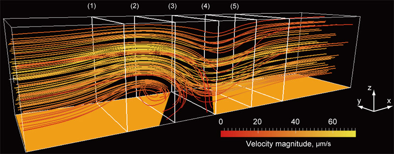
3D ACET flow in a microchannel
1. Introduction
Mass transport over reactive solid surfaces is a widely used physical and chemical phenomenon that forms the basis of several engineering, biochemical, and medical applications. Biosensors used in immunoassays have been developed to investigate surface modifications, antibody–antigen binding, and deoxyribonucleic acid hybridization without fluorescent labeling 1. The efficiency of surface reactions is determined not only by the association and dissociation kinetics of the binding process but also by mass transport kinetics, including convective transport in the surrounding fluid. In microfluidic systems, miniaturization increases the surface-to-volume ratio and potentially improves reaction throughput; however, the Peclet number decreases with a decrease in system size, resulting in diffusion-dominated transport conditions. In such diffusion-limited regimes, externally induced convective flow toward the reactive interface is effective in enhancing mass transport and improving surface reaction efficiency.
In addition to mass transport, the flow structure near the substrate is crucial for regulating the mechanical microenvironment of cells cultured in microfluidic devices. Fluid motion near the wall generates hydrodynamic shear stress that directly affects cell adhesion, morphology, proliferation, differentiation, and signal transduction 2,3. Consequently, microfluidic platforms have been widely used not only to deliver biochemical stimuli but also to impose well-defined mechanical stimuli on cells, driving the quantitative studies on cell adhesion and mechanobiology 4,5. Thus, the local flow field should be considered a critical design parameter when microfluidic systems are used for sensor-based information acquisition from cells and tissues because it directly affects analyte delivery, sensor response, and cellular behavior. In this context, the quantitative characterization of 3D near-wall flows is essential to evaluate how active flow modulation affects the sensing performance at reactive interfaces and mechanical stimulation applied to cultured cells.
The active modulation of fluid motion by external fields is a promising strategy to control transport and mechanical environments in microfluidic systems. Among various actuation methods, alternating current (AC) electrokinetic (ACEK) phenomena are attractive because fluid motion can be generated and tuned locally by adjusting electrode geometry, applied voltage, and frequency without requiring mechanical pumps or moving components. ACEK-based actuation has been used to induce microscale mixing, pumping 6, and particle manipulation 7. In addition, AC electrothermal (ACET) flow, which is an ACEK mechanism, can operate effectively in relatively high-conductivity liquids because it originates from Joule heating-induced gradients in electrical properties under an applied electric field 8. This feature is advantageous for biological and cell-related microfluidic applications where culture media and physiological buffers have higher ionic conductivities than dilute electrolyte solutions. Recently, on-chip ACET chips have been developed to demonstrate the pulsatile perfusion of human mesenchymal stem cells 9. ACET flows often have 3D structures near the electrodes and walls, and quantitative 3D characterization is necessary to evaluate their actual effect on surface reactions, sensor responses, and cellular stimulation.
Micron-resolution particle image velocimetry (micro-PIV) reported by Santiago et al. 10 has become an essential tool to measure velocity profiles in microfluidic systems. Thus far, several techniques have been proposed to extend the capability of micro-PIV. Ensemble averaging of the cross-correlation function in image processing 11 improves spatial resolution and measurement accuracy under steady flow conditions. However, conventional micro-PIV has an inherent limitation in that the measurable velocity field is two-dimensional (2D) with two velocity components (2D–2C). To overcome this limitation and obtain full three-dimensional velocity information (3D–3C), several advanced measurement techniques have been developed to investigate microscale fluid dynamics.
Stereoscopic micro-PIV 12 can measure all three velocity components in a 2D observation plane using a stereoscopic microscope with dual optical paths to observe the measurement region from two different viewing angles. The three velocity components are reconstructed by combining displacement vectors obtained from the two views using a mapping and calibration process. The successful application of stereoscopic micro-PIV was demonstrated for 3D flow in a T-shaped micromixer 12. Bown et al. 13 validated the experimentally measured 3D flow over a microscale backward-facing step through comparison with computational fluid dynamics results. Another approach to 3D velocity measurement is holographic micro-PIV. Holography can record volumetric flow information by storing interference patterns of light in a photosensitive medium. Yang and Chuang developed the first holographic micro-PIV system using multiplexed optical holography 14, whereas Kim and Lee used digital holography to measure laminar flow in a microtube 15. Moreover, Ooms et al. applied holographic techniques to a T-shaped micromixer 16. Although these holographic methods provide true volumetric flow measurements, they require complex optical setups and computationally intensive reconstruction procedures; furthermore, the resolution of out-of-plane velocity components remains lower than that of in-plane components. The use of defocused particle images to extract depth information has become a powerful approach for 3D particle tracking in microfluidics 17. Among these techniques, astigmatism particle-tracking velocimetry (PTV) has attracted considerable attention because it can estimate the out-of-plane position of tracer particles from a single camera view by intentionally introducing optical aberration into the imaging system. Using a cylindrical lens, the particle image shape becomes depth-dependent, enabling 3D particle positions and velocities to be reconstructed with a relatively simple optical setup compared to those of stereoscopic or holographic methods 18. Although astigmatic PTV provides a compact approach for 3D particle tracking, its performance is highly sensitive to calibration quality, signal-to-noise ratio, particle image characteristics, and seeding density, which limit the accuracy of depth reconstruction.
In this study, a 3D velocity measurement method based on twin-view scanning 2D–2C micro-PIV with orthogonal observation planes was developed. This method reconstructs the 3D velocity field by combining velocity measurements obtained from two orthogonal planes. All three velocity components of laminar flow in a tilted straight microchannel were measured to evaluate the validity of this technique. Furthermore, the 3D flow field induced by ACEK phenomenon, specifically ACET flow, was investigated. The 3D flow structure generated by ACET was analyzed to evaluate its contribution to enhanced mass transport toward the reactive surface and to the generation of localized shear stimulation near the substrate. These results demonstrate the potential of ACET-driven flow to simultaneously enhance surface reactions and regulate cellular mechanical environments in microfluidic systems.
2. Orthogonal-Plane Micro-PIV
Micro-PIV determines the 2D–2C velocity field from successive images of fluorescent tracer particles recorded within the focal plane of a microscope objective 10,19. The most straightforward approach to extend the measurement dimension is to use a scanning scheme along the direction normal to the focal plane. The volumetric distribution of the in-plane velocity components can be obtained by sequentially acquiring velocity fields at different focal depths. However, this method provides only two velocity components at each measurement plane and does not directly yield the out-of-plane velocity component.
In this study, a pair of measurement planes intersecting orthogonally was employed to obtain the out-of-plane velocity component and reconstruct the 3D–3C velocity field. An arbitrary velocity vector \(\mathbf{u}\) in 3D Euclidean space can be expressed as
By projecting this velocity vector onto planes formed by combinations of orthogonal basis vectors, projected velocity fields in the \(xy\)-, \(yz\)-, and \(xz\)-planes can be expressed as
These projections confirm that all three components of the original velocity vector can be determined from at least two projected vectors obtained from orthogonal observation planes.
Two scanning micro-PIV measurements were performed independently using orthogonal focal planes to reconstruct the 3D velocity field within the measurement volume. Fig. 1 illustrates the configuration of measurement planes corresponding to the \(xy\)- and \(xz\)-views. The \(xy\)-plane observation was performed through the bottom of the microfluidic device with the focal plane parallel to the channel wall, while the \(xz\)-plane observation was conducted through the sidewall of the channel with the focal plane perpendicular to the substrate.
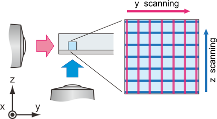
Fig. 1. Schematic of 3D velocimetry using orthogonal-plane micro-PIV. 3D–3C information of a velocity field in a microchannel can be obtained by orthogonal twin-view observation and focal-plane scanning.
The measurement volume was discretized into a predefined regular grid for facilitating post-processing and data merging. Velocity components obtained from each observation plane were linearly interpolated onto grid points. The bottom and sidewalls of the channel were used as reference features to define a common coordinate system. The overlapping \({u}\)-components obtained from both views were averaged to minimize measurement uncertainty. Consequently, the reconstructed 3D velocity field with three velocity components (\({u}\), \({v}\), \({w}\)) was obtained as
The \(xy\)- and \(xz\)-plane measurements were performed independently and sequentially. Therefore, the reconstructed 3D–3C velocity field assumes that the flow field remains steady during the acquisition of both orthogonal views. In this study, the pressure-driven flow conditions, applied AC voltage, and frequency were kept constant during measurements, and the velocity fields used for reconstruction were obtained after the flow reached a steady state. The flow regime in this study is laminar, and therefore, flow fluctuations are considered negligible.
3. Experimental Setup
3.1. Microfluidic Device
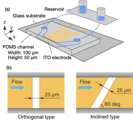
Fig. 2. Schematic of microfluidic device. (a) Bird’s-eye view and (b) electrode geometries on the bottom substrate.
A schematic of the microfluidic device used in this study is shown in Fig. 2(a). The device consists of a polydimethylsiloxane (PDMS) microchannel bonded to a glass substrate with patterned coplanar electrodes. The PDMS microchannel has a straight rectangular cross-section with a width and height of 100 and 50 μm, respectively.
For the optical observation of fluorescent particles through the sidewall of the channel, the wall must be sufficiently thin and optically flat. The sidewall thickness is set to 117 μm, which is optimized to obtain clear particle images without leakage. The outer surface of the sidewall is fabricated to be as flat as a coverslip because it is commonly used as the bottom substrate in micro-PIV measurements. During the molding process in softlithography, a flat glass plate was used as part of the mold to achieve the required surface flatness. In addition, an objective lens with a correction collar is used to reduce spherical aberration caused by differences in the optical path length between the sample and objective lens. The \(xy\)- and \(xz\)-plane observations through the glass substrate and PDMS sidewall exhibit different optical paths; therefore, the correction collar is adjusted for each observation direction to improve the particle-image quality. This adjustment is important for reducing view-dependent optical aberrations in the sidewall observation.
The electrodes were fabricated from indium tin oxide (ITO) by sputtering and patterned using a wet-etching process. The ITO film is highly transparent in the visible wavelength range; therefore, optical measurements can be performed through a glass substrate with ITO pattern beneath the microfluidic device. Two types of electrode patterns were used, as shown in Fig. 2(b). One pattern has an electrode gap oriented perpendicular to the direction of the main flow, while the other has an inclined gap with an angle of 60° relative to the main flow direction.
Ultrapure Milli-Q water and an aqueous KCl solution were used as the working fluids to measure pressure-driven laminar and electrokinetic flows, respectively. The pressure drop in the microchannel was generated by the difference in liquid levels between the inlet and outlet reservoirs. The electrical conductivity of the KCl solution (Wako) was adjusted to 1.5 S/m. Fluorescent polystyrene particles with a diameter of 0.5 μm (Fluoro-Max G500, ThermoFisher) were added as tracer particles. The excitation and emission wavelengths of the fluorescent particles were 505 and 515 nm, respectively.
3.2. Measurement System and Procedure
Figure 3 illustrates the schematic of the experimental setup. The measurement system was based on an inverted microscope equipped with common components for fluorescence imaging, including an objective lens, a filter set, an illumination source, a camera, and a motorized stage.
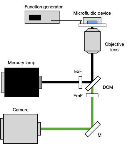
Fig. 3. Measurement system used in this study.
The objective lens (Nikon, CFI Plan Fluor 40\(\times\)) had a magnification of 40\(\times\) and a numerical aperture of 0.6. A continuous mercury lamp (Nikon, C-HGFL) was used as an illumination source. Fluorescence emitted from tracer particles was recorded using a scientific complementary metal-oxide-semiconductor camera (Hamamatsu, ORCA-Flash2.8) with a pixel size of 3.63 μm, an image resolution of \(1920 \times 1440\) pixels, and a 16-bit dynamic range. The target stage was controlled to scan the focal plane with a positioning accuracy of 0.1 μm. Electrodes on the bottom wall of the microfluidic device were connected to a function generator (Tektronix, AFG3102) to apply an AC voltage with controlled amplitude and frequency (5–10 V\(_\textrm{p-p}\) at 1 MHz).
In the correlation-based micro-PIV analysis, the calculated particle displacement represents the spatially averaged displacement of tracer particles within an interrogation window. The measurement plane in micro-PIV has a finite depth determined by the optical characteristics of the imaging system. Therefore, the interrogation region can be considered a measurement volume. In the present experiments, the measurement depth 20 was 7 μm based on the optical parameters of the objective lens and fluorescence wavelength. The remaining analysis parameters were set similar to those used in conventional micro-PIV. The horizontal spatial resolution defined by the interrogation window size used in the correlation analysis was set to \(7.08 \times 7.08\) μm\(^2\), which is comparable to the measurement depth. Therefore, the spatial resolution of the reconstructed 3D–3C velocity field can be considered nearly isotropic.
Fluorescent images were acquired under low-particle-concentration conditions to improve the signal-to-noise ratio of recorded images. Before the correlation analysis, background noise reduction and image superposition were performed to enhance particle visibility. Finally, 100 instantaneous velocity fields were averaged to reduce uncertainty caused by the inherent Brownian motion of tracer particles in the fluid.
4. Results and Discussion
4.1. Verification of 3D Velocity Reconstruction
In this study, the validity of the developed orthogonal-plane micro-PIV technique was verified prior to the measurement of electrokinetic flow under an AC electric field in the microfluidic device. As a preliminary experiment, a tilted rectangular microchannel was employed as a reference flow. In this configuration, the microfluidic device was tilted with respect to the \(z\)-axis, as illustrated in Fig. 4. Subsequently, the focal plane of the objective lens was scanned along the depth direction to obtain the volumetric velocity field.
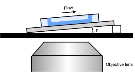
Fig. 4. Tilted arrangement of the microchannel for the preliminary validation of the orthogonal-plane micro-PIV.
The analytical solution of the streamwise velocity \(u_{0}(y,z)\) for fully developed laminar flow in a rectangular straight channel without tilt is given as 21
In a simple pressure-driven flow in a horizontally aligned microchannel, only the streamwise velocity component is nonzero. However, a \({z}\)-component of velocity \({w}\) appears and increases with increasing tilt angle when the channel is tilted by an angle \(\gamma\) with respect to the \({z}\) direction. Therefore, velocity components in the tilted channel (\(u_{\gamma}\), \(w_{\gamma}\)) can be expressed as
Figure 5 shows the velocity distribution measured in the center plane of the microchannel. The circles represent the experimentally measured velocities, while the solid line represents the analytical laminar velocity profile calculated using Eqs. (7) and (8), respectively. In this experiment, the pressure gradient \({dp}/{dx}\) was not directly measured; however, fitting the analytical velocity distribution to the measured velocity profile using \({dp}/{dx}\) as a fitting parameter is sufficient to evaluate measurement accuracy 21.
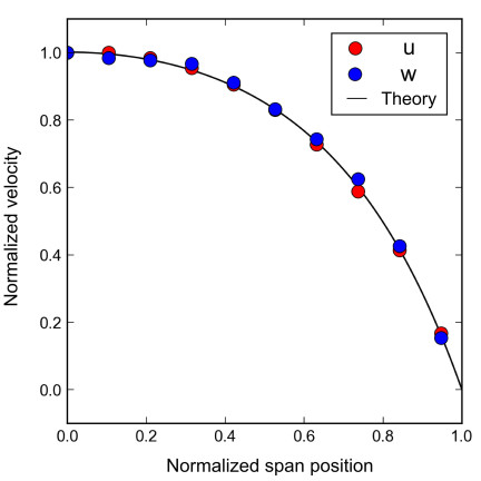
Fig. 5. Velocity profile in a rectangular straight channel with a tilt angle of 2.6° with respect to the \(z\) direction. Plots and lines represent measured results and fitted analytical solutions, respectively.
Experimental results agreed well with the analytical solutions, with deviations of 3.8% and 5.5% for the \({u}\) and \(w\) components, respectively. These deviations are smaller than the typical measurement uncertainty reported in the literature, which is \(\sim\)10% 13. Moreover, the tilt angle estimated from measured velocity components was in good agreement with the actual tilt angle of 2.64°. These results confirm the validity of the orthogonal-plane micro-PIV technique for 3D velocity measurements in microfluidic platforms.
4.2. Characterization of AC Electrothermal Flow
The ACET effect is a fluid motion induced by ACEK phenomena. Under an AC electric field, the fluid is locally heated by Joule dissipation, which produces spatial gradients in the electrical conductivity and permittivity of the fluid because of their intrinsic temperature dependence. In the presence of these property gradients and an applied electric field, an electrohydrodynamic body force acts on the fluid, resulting in ACET flow. According to theory 8, the ACET body force \(\mathbf{F}_{ET}\ \)can be expressed as
The volumetric heat generation in the fluid caused by Joule heating can be expressed as
Joule heating becomes more significant in conductive liquids; therefore, ACET flow is effectively generated in relatively high-conductivity solutions. The characteristic ACET velocity is proportional to the fourth power of the applied voltage \({V}\). Under the present experimental conditions, the temperature increase in the fluid is \(\sim\)1 K, indicating that the effects of heating on the electrolysis, evaporation, and chemical degradation are negligible.
Side-view measurements are performed using an orthogonal electrode device to observe the fundamental 2D structure of ACET flow. Fig. 6 shows the velocity field in the \({xz}\)-plane at the spanwise center of the channel under an applied voltage of 9 V\(_\textrm{p-p}\) at 1 MHz. A circular stirring flow was observed along the electrode gap, conveying fluid from the bulk region to the bottom surface of the microchannel. The flow field results from the superposition of the pressure-driven main and ACET flows. For the velocity field shown in Fig. 6, pressure-driven and ACET flows are considered to be of the same order of magnitude, resulting in the observed wavy flow pattern with rotational flow structures; this reflects a comparable contribution of ACET. The contribution of this vertical transport represented by the \({z}\)-component velocity is induced by the electric field; therefore, the average \(z\)-component velocity in the region \(-5 < x < 5\) μm and \(15 < z < 25\) μm was evaluated to quantify the voltage dependence of ACET flow. As shown in Fig. 7, the measured velocity followed a power-law dependence on the applied voltage with an exponent of 4.01, which is in excellent agreement with the theoretical \({V}^{4}\) scaling because Joule heating scales with \({V}^{2}\) and the electrohydrodynamic body force scales with \({E}^{2}\).
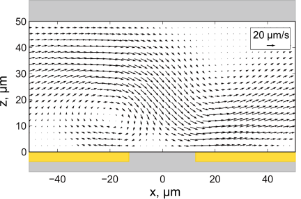
Fig. 6. ACET flow field with the applied voltage of 9 V\(_\textrm{p-p}\) and at a frequency of 1 MHz over an electrode gap placed perpendicular to the mainstream.
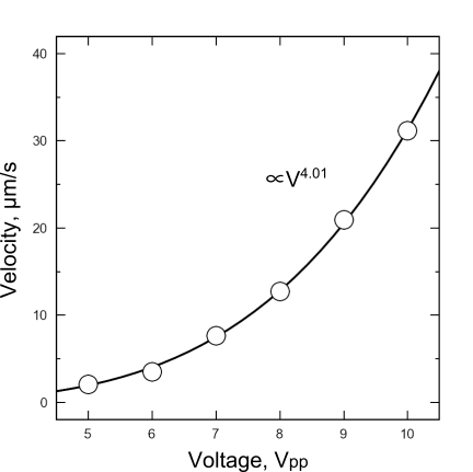
Fig. 7. Measured \(z\)-component velocity of ACET flow under different voltages from 5 to 10 V\(_\textrm{p-p}\) and correlation with the power law.
Furthermore, this result indicates that the observed flow was dominated by ACET rather than by other ACEK phenomena. For example, AC electroosmosis (ACEO) and dielectrophoresis (DEP) scale with the square of the applied voltage \({V}^{2}\). In addition, ACEO is prominent at considerably lower frequencies in the order of several kilohertz 22, whereas the experiments in this study were performed at 1 MHz. Under this condition, the DEP-induced motions of tracer particles were negligibly small. Therefore, the contribution of other ACEK mechanisms can reasonably be neglected.
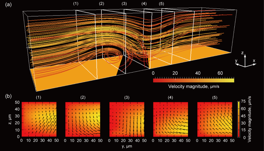
Fig. 8. 3D flow structure of ACET over an inclined-electrode-gap device with an applied voltage of 10 V\(_\textrm{p-p}\) at a frequency of 1 MHz. (a) Streamlines showing characteristic circular motion and (b) velocity fields at each cross-section.
A strong 3D ACET flow was generated in the channel when the inclined electrode geometry was employed. Fig. 8(a) shows the reconstructed 3D flow field in an inclined-electrode device at 10 V\(_\textrm{p-p}\) and 1 MHz; only half of the channel width is shown. A characteristic stirring motion was observed along the inclined electrode gap, and the inclination of the electrode introduced an additional spanwise component of fluid motion, as shown in Fig. 8(b). Consequently, the overall flow field was formed by the superposition of the pressure-driven laminar mainstream and inclined ACET-induced secondary flow.
In terms of mass transport, this 3D stirring motion enhanced the delivery of suspended analytes from the bulk fluid toward the reactive surface or adhered cell. The additional spanwise and wall-normal transport reduced local transport limitations near the bottom and increased the probability of interaction between suspended species and immobilized molecules on the surface. This mechanism explains the enhancement in the surface reaction efficiency induced by ACEK actuation.
Meanwhile, the present results suggest an additional implication for cell-based microfluidic systems. The ACET-induced flow introduces wall-normal recirculation and modifies the near-wall velocity gradient, and therefore, it locally alters the shear environment experienced by cells cultured on the substrate. Thus, the 3D flow structure that enhances surface transport can also provide localized mechanical stimulation to adherent cells through shear stress. The near-wall shear rate was estimated from the velocity distribution shown in Fig. 8. The inclined ACET flow increased the maximum near-wall velocity gradient by up to approximately twofold compared with the condition without voltage application. This is important in microphysiological systems and cell culture platforms, where cellular behavior is strongly affected not only by biochemical transport but also by hydrodynamic stimuli. A recent study 9 demonstrated that ACET flow modulation can enhance the osteogenic differentiation of human mesenchymal stem cells by generating pulsatile stimulation of adherent cells on a chip. However, the underlying 3D flow structure has not been characterized.
Consequently, the reconstructed 3D–3C velocity field is valuable for understanding reaction enhancement by ACEK flow and for quantitatively discussing how flow modulation by the ACEK effect contributes to localized shear stimulation near the culture surface.
5. Conclusion
A 3D–3C velocity measurement technique based on orthogonal observation planes combined with focal-plane scanning was developed. The validity of the proposed method was verified by comparing the measured velocity field in a tilted rectangular microchannel with the corresponding analytical solution for fully developed laminar flow. The maximum deviations for the horizontal and vertical velocity components were 3.8% and 5.5%, respectively, demonstrating the sufficient accuracy of the proposed technique for 3D flow measurements in microfluidic systems.
Using this method, the 3D velocity field of ACET flow was measured successfully. The results revealed that electrode geometry induced electrokinetically driven spanwise and wall-normal convective motions, resulting in a characteristic 3D stirring flow in the channel. Such flow distortion enhances analyte transport from the bulk toward the substrate and promotes localized reactions, indicating the strong potential of AC electrokinetic actuation for improving surface reaction efficiency.
Moreover, the results suggest that AC electrokinetic flow can modify the near-wall hydrodynamic environment and mass transport. The wall-normal recirculation and locally enhanced velocity gradients generated by ACET flow are expected to contribute to the localized shear stimulation on cells cultured on the substrate. Therefore, the present 3D–3C measurement approach provides a useful tool not only for evaluating transport enhancement in surface reactions but also for understanding and designing electrokinetically controlled mechanical microenvironments in microfluidic cell culture systems.
Acknowledgments
This work was financially supported by JSPS KAKENHI (Grant Number JP 25K01179). Part of the microfabrication was supported by the “Advanced Research Infrastructure for Materials and Nanotechnology in Japan (ARIM)” of the Ministry of Education, Culture, Sports, Science, and Technology (MEXT) (Proposal number JPMXP1224UT1163).
- [1] S. Scarano, M. Mascini, A. P. F. Turner, and M. Minunni, “Surface plasmon resonance imaging for affinity-based biosensors,” Biosensors and Bioelectronics, Vol.25, No.5, pp. 957-966, 2010. https://doi.org/10.1016/j.bios.2009.08.039
- [2] G. Chen, Y. Lv, P. Guo, C. Lin, X. Zhang, L. Yang, and Z. Xu, “Matrix mechanics and fluid shear stress control stem cells fate in three dimensional microenvironment,” Current Stem Cell Research & Therapy, Vol.8, No.4, pp. 313-323, 2013. https://doi.org/10.2174/1574888X11308040007
- [3] C. P. Gayer and M. D. Basson, “The effects of mechanical forces on intestinal physiology and pathology,” Cell Signalling, Vol.21, No.8, pp. 1237-1244, 2009. https://doi.org/10.1016/j.cellsig.2009.02.011
- [4] W. J. Polacheck, R. Li, S. G. M. Uzel, and R. D. Kamm, “Microfluidic platforms for mechanobiology,” Lab on a Chip, Vol.13, No.12, pp. 2252-2267, 2013. https://doi.org/10.1039/C3LC41393D
- [5] H. Lu, L. Y. Koo, W. M. Wang, D. A. Lauffenburger, L. G. Griffith, and K. F. Jensen, “Microfluidic shear devices for quantitative analysis of cell adhesion,” Analytical Chemistry, Vol.76, No.18, pp. 5257-5264, 2004. https://doi.org/10.1021/ac049837t
- [6] X. Gao and Y. Li, “Biofluid pumping and mixing by an AC electrothermal micropump embedded with a spiral microelectrode pair in a cylindrical microchannel,” Electrophoresis, Vol.39, Issue 24, pp. 3156-3170, 2018. https://doi.org/10.1002/elps.201800162
- [7] A. Abdelghany, K. Yamasaki, Y. Ichikawa, and M. Motosuke, “Efficient nanoparticle focusing utilizing cascade AC electroosmotic flow,” Electrophoresis, Vol.43, Issues 16-17, pp. 1755-1764, 2022. https://doi.org/10.1002/elps.202200054
- [8] A. Ramos, H. Morgan, N. G. Green, and A. Castellanos, “AC electrokinetics: a review of forces in microelectrode structures,” J. of Physics D: Applied Physics, Vol.31, pp. 2338-2353, 1998. https://doi.org/10.1088/0022-3727/31/18/021
- [9] I. Kawata, S. Kobayashi, Y. Ichikawa, and M. Motosuke, “On-chip AC electrothermal pump for pulsatile perfusion,” Micromachines, Vol.17, No.4, Article No.492, 2026. https://doi.org/10.3390/mi17040492
- [10] J. G. Santiago, S. T. Wereley, C. D. Meinhart, D. J. Beebe, and R. J. Adrian, “A particle image velocimetry system for microfluidics,” Experiments in Fluids, Vol.25, pp. 316-319, 1998. https://doi.org/10.1007/s003480050235
- [11] C. D. Meinhart, S. T. Wereley, and J. G. Santiago, “A PIV algorithm for estimating time-averaged velocity fields,” J. of Fluids Engineering, Vol.122, No.2, pp. 285-289, 2000. https://doi.org/10.1115/1.483256
- [12] R. Lindken, J. Westerweel, and B. Wieneke, “Stereoscopic micro particle image velocimetry,” Experiments in Fluids, Vol.41, pp. 161-171, 2006. https://doi.org/10.1007/s00348-006-0154-5
- [13] M. R. Bown, J. M. MacInnes, R. W. K. Allen, and W. B. J. Zimmerman, “Three-dimensional, three-component velocity measurements using stereoscopic micro-PIV and PTV,” Measurement Science and Technology, Vol.17, pp. 2175-2185, 2006. https://doi.org/10.1088/0957-0233/17/8/017
- [14] C.-T. Yang and H.-S. Chuang, “Measurement of a microchamber flow by using a hybrid multiplexing holographic velocimetry,” Experiments in Fluids, Vol.39, pp. 385-396, 2005. https://doi.org/10.1007/s00348-005-1022-4
- [15] S. Kim and S. J. Lee, “Measurement of 3D laminar flow inside a micro tube using micro digital holographic particle tracking velocimetry,” J. of Micromechanics and Microengineering, Vol.17, No.10, pp. 2157-2162, 2007. https://doi.org/10.1088/0960-1317/17/10/030
- [16] T. A. Ooms, R. Lindken, and J. Westerweel, “Digital holographic microscopy applied to measurement of a flow in a T-shaped micromixer,” Experiments in Fluids, Vol.47, pp. 941-955, 2009. https://doi.org/10.1007/s00348-009-0683-9
- [17] R. Barnkob and M. Rossi, “General defocusing particle tracking: fundamentals and uncertainty assessment,” Experiments in Fluids, Vol.61, Article No.110, 2020. https://doi.org/10.1007/s00348-020-2937-5
- [18] Y. Ichikawa, R. Kikuchi, K. Yamamoto, and M. Motosuke, “Determining particle depth positions and evaluating dispersion using astigmatism PTV with a neural network,” Applied Optics, Vol.60, Issue 22, pp. 6538-6546, 2021. https://doi.org/10.1364/AO.427571
- [19] C. D. Meinhart, S. T. Wereley, and J. G. Santiago, “PIV measurements of a microchannel flow,” Experiments in Fluids, Vol.27, pp. 414-419, 1999. https://doi.org/10.1007/s003480050366
- [20] C. D. Meinhart, S. T. Wereley, and M. H. B. Gray, “Volume illumination for two-dimensional particle image velocimetry,” Measurement Science and Technology, Vol.11, No.6, pp. 809-814, 2000. https://doi.org/10.1088/0957-0233/11/6/326
- [21] F. M. White, “Viscous Fluid Flow,” p. 123, McGraw-Hill, 1974.
- [22] M. Motosuke, K. Yamasaki, A. Ishida, H. Toki, and S. Honami, “Improved particle concentration by cascade AC electroosmotic flow,” Microfluidics and Nanofluidics, Vol.14, No.6, pp. 1021-1030, 2013. https://doi.org/10.1007/s10404-012-1109-1
This article is published under a Creative Commons Attribution-NoDerivatives 4.0 Internationa License.