
Paper:
Obstacle Avoidance Using Population Vector Code-Based SNN-CPG Controller for Robotic Fish in Unknown Environment
Takumi Asada*
 , Hideo Furuhashi**
, Kenta Tabata*
, Renato Miyagusuku*
, and Koichi Ozaki*
, Hideo Furuhashi**
, Kenta Tabata*
, Renato Miyagusuku*
, and Koichi Ozaki*
*Graduate School of Engineering, Utsunomiya University
7-1-2 Yoto, Utsunomiya, Tochigi 321-8585, Japan
**Department of Electronics and Electrical Engineering, Aichi Institute of Technology
1247 Yachigusa, Yakusa-cho, Toyota, Aichi 470-0392, Japan

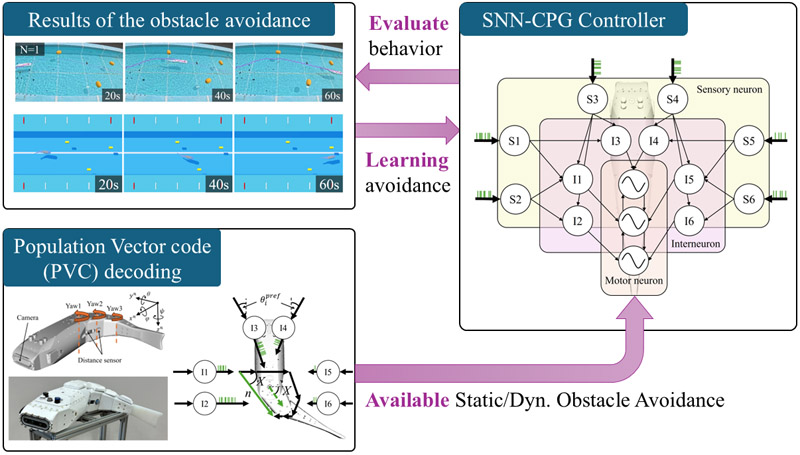
Neurorobotics, which incorporates neuromorphic computing into robotic systems, can emulate biological intelligence and behaviors. The characteristics of neural responses and behavioral patterns are reproduced using spiking neural networks. Many applications utilize mobility robots; however, applications with multiple joints, such as robotic fish, remain limited. The main challenge is that shape types and joint numbers vary among biological organisms, and disturbances affect them in underwater environments. The neural circuit mechanisms used by multi-jointed robots for obstacle avoidance have not yet been clarified. In this study, we propose an obstacle avoidance architecture realized exclusively through neural circuits. The fundamental obstacle avoidance performance of a robotic fish was systematically evaluated, including ablation studies, varying conditions, and the physical environment.
Conceptual overview of PVC-based SNN-CPG controller
1. Introduction
In vertebrates, locomotor neural circuits are distributed throughout the spinal cord, midbrain, and higher brain regions. The spinal cord plays a crucial role in locomotor control by utilizing central pattern generators (CPGs) and multiple reflex loops that provide feedback mechanisms 1. Stimulation of the midbrain activates locomotor output scaling with stimulation intensity 2. This feature is evolving as an integration of neuromorphic and robotic technologies 3. Neurorobotics development studies have focused on the utilization of neuromorphic computing and spiking neural networks (SNNs) in robotic applications 4. SNNs are composed of neural models based on local learning rules, event-driven processing, spike-based binary communication, and biological synaptic plasticity. These characteristics have attracted attention as computational models for SNNs that have low power consumption and computational cost, and closely resemble biological neural systems. Learning capabilities also enable mobile and biomimetic robots to acquire adaptive control and behavior. Their ability to adjust synaptic connections enables complex task performance and behavioral learning 5,6,7. Obstacle avoidance using SNNs has been attempted in behavioral tasks. The use of LiDAR data enables obstacle avoidance based on SNNs and kinematic state vectors that are directly mapped to robot commands 8. A neuromorphic vision sensor-based deep reinforcement learning (DRL) approach using SNNs achieved dynamic obstacle avoidance 9. Biologically-motivated SNNs have been evaluated for goal-directed collision avoidance 10. SNN-based obstacle avoidance is primarily utilized in mobile robot applications, with limited use in robotic fish applications. Many obstacle-avoidance systems for fish-like robots require that avoidance scenarios and models be defined in advance 11. Motion control technology has been implemented in robotic fish using SNN and CPG to enable adaptation to different scenarios 12,13. The actions acquired also depend on the number of joints (multi-joint) and the shape type (caudal or pectoral fin) of the robotic fish. Neural circuitry also differs depending on the joint structure. Additionally, obstacle avoidance using SNNs is a challenging task in underwater environments owing to disturbances such as waves. Closed-loop control with feedback from sensory inputs enables various movement patterns and the avoidance of static and dynamic obstacles 14. Therefore, it is crucial for SNN-based systems to incorporate the robot’s shape, joint configuration, and sensor inputs.
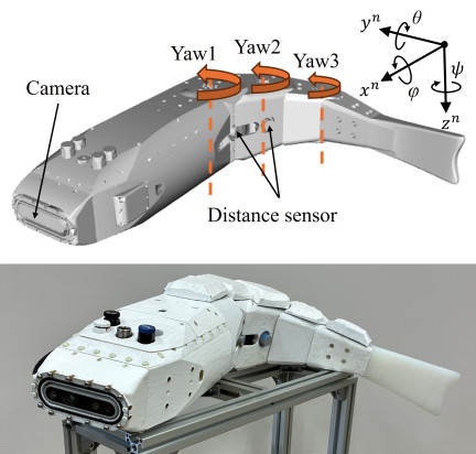
Fig. 1. Model of the robotic fish.
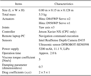
Table 1. Technical specifications of the robotic fish.
To achieve obstacle avoidance using SNNs in a robotic fish, we propose a population vector code (PVC)-based SNN-CPG method. Population vector algorithm converts neural activity from external stimuli into behavior, contributing to object localization 15,16. The neural representation of external stimuli in space-time enables the construction of neuromorphic architectures in SNNs. In addition, SNNs can adaptively update synaptic weights by learning rules via hierarchization. This enables the acquisition of obstacle avoidance behaviors in response to environmental changes. The contribution of this study is the evaluation of the performance of a three-layer architecture combining the PVC and SNN-CPG for obstacle avoidance. Obstacle avoidance performance was evaluated according to the preferred direction of the PVC, with or without SNN training. The effectiveness of the proposed method is demonstrated experimentally using physical hardware and simulation environment.
2. Modeling of the Robotic Fish
2.1. Hardware Modeling
The robotic fish used to evaluate the proposed method is shown in Fig. 1, and its specifications are listed in Table 1. The dimensions of the robot are 0.80 m in length, 0.15 m in width, and 0.128 m in height. The robotic fish had three yaw-axis joints in the tail fin. The total weight of the model was set to 5.5 kg, and it was designed to float on water. The viscous torque, damping, and drag force coefficients were specified by the designer, considering previous Sim2Real evaluation studies 17 and the robot model size. The fluid dynamics model used in the simulation assumed a laminar flow with uniform density, viscosity, and flow velocity. Flow phenomena such as turbulence and vortex shedding were not explicitly modeled. To improve the expected accuracy of both the simulation and the physical robot, the fluid dynamic parameters were adjusted based on experiments of fundamental movements performed by physical robot. Therefore, it is assumed that the gap between the physical and model parameters is small. The robot is equipped with a camera mounted on the head component and four distance sensors on the lateral components, with two sensors on each side. The distance sensor is an ultrasonic type with a measurement range of 0.02–3.0 m and a field of view of 5°–10°. The input image is divided into left and right frames. The shortest distance between the camera and the object detected within the frame is used as the distance measurement for the left and right sides. Distance values were corrected for underwater measurements. Six inputs comprising the left and right frames from the camera and four distance sensors were used as inputs for the sensory neurons.
2.2. Robotic Fish Dynamics and Kinematics
The dynamics of a robotic fish use Fossen’s model, which is widely applied in underwater robotics. This study considers the motion in a three-degree-of-freedom (3-DOF) system (surge, sway, yaw), following Fossen’s model 18. The added mass and drag matrix terms in Fossen’s model are assumed to follow Lamb’s k-factor definition 19. The kinematic model of a fish robot with three yaw-axes has been widely used in the literature 20,21; therefore, this robot adopts the existing formulation, and focuses on the proposed control framework.
3. Hierarchical SNN Architecture
Figure 2 shows the SNN configuration, which imitates the locomotor neural circuits of a robotic fish. These consist of three-layers: sensory neurons that detect external stimuli, interneurons that connect the sensory and motor systems, and motor neurons that generate motor outputs.
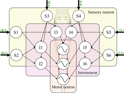
Fig. 2. Diagram of hierarchical SNN architecture.
3.1. Rate Encoding for Sensory Neurons
The external stimuli are encoded by sensory neurons as Poisson spike trains. To account for uncertainty, sensory noise, and the neural effective refractory period, we use a Poisson process with dead-time (PPD) 22. The standard Poisson process is as follows:
3.2. Spiking Neuron Model for Interneurons
The spikes from each sensory neuron are integrated into the interneurons and converted into motor outputs. Each neuron is connected to other neurons via excitatory synapses, as shown in Fig. 2, and bilaterally symmetrical inhibitory synapses. The input spike excites the synapse. We define the synaptic input as the sum of the post-synaptic currents (PSCs) as follows:
Interneurons use the Izhikevich model to integrate post-synaptic currents and generate diverse spike firing patterns 24. The membrane potential \(v_i\) and recovery variable \(u_i\) of the \(i\)-th interneuron can be expressed as follows:
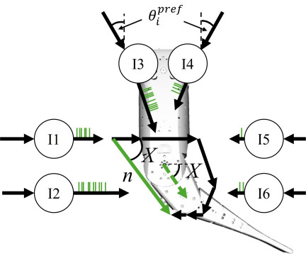
Fig. 3. PVC-based decoding of motor neuron output.
3.3. Population Vector Code for Motor Neurons
Spike trains are integrated and decoded in the PVC, and utilized for motor neuron output. We focused on the property that stimulus responses differ depending on the preferred direction 25. Fig. 3 shows the calculation method for the PVC and its effect on motor neurons. The population vector \(\mathbf{n}\) for the entire system can be defined as the set of preferred direction vectors \(\mathbf{e}_i\), and the momentary firing rates \(v_i\), of each neuron:
The population vector determined by the PVC is decoded and outputted to the motor neuron as follows:
3.4. Learning SNN with r-STDP
The three-layer architecture utilizes SNN learning rules to enable obstacle avoidance in unknown environments. Spike-timing-dependent plasticity (STDP) is a Hebbian-based learning rule for SNNs. The idea of implementing biological RL is reward modulated STDP (r-STDP) 29, which adjusts the determined weights and demonstrates superior performance compared with STDP 30. Therefore, the synaptic weights between sensory neurons and interneurons are designed to be enhanced or weakened via the r-STDP rules to achieve optimal weights for obstacle avoidance.
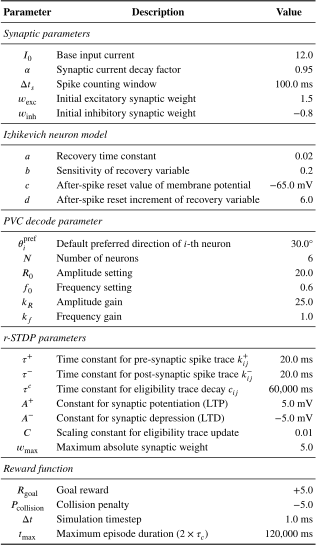
The architecture adapting PVC to the SNN-CPG structure is a novel method capable of consistently reproducing the neural circuitry from external stimuli to the motor output. The ability to adapt to obstacle avoidance by learning the synaptic connection strength between sensory neurons and interneurons using the r-STDP rule was evaluated.
Table 2. Parameters of hierarchical SNN architecture.
4. Simulation Evaluation of Architecture
4.1. Preparing the Verification Environment
The proposed method was validated in an underwater simulation environment of Webots. The simulation environment is illustrated in Fig. 4. The underwater experimental pool was 6 m long, 2 m wide, and 0.45 m deep. In this experiment, we focused on motion in the horizontal plane (\(x\)-\(y\) plane) and did not consider motion in the vertical direction. The robot was positioned at the center of the yellow start area and maneuvered toward the red target area, 4 m ahead. External stimuli are transmitted to motor neurons via interneurons, obstacles are identified, and propulsion is executed through neural circuits alone. Dynamic obstacles were placed in the regions around \((2,0.5)\) and \((4,-0.5)\), with the start position set to \((x,y)=(0,0)\) as shown in Fig. 4(a). The dynamic obstacles were modeled as a school of fish-like agents moving at a constant speed of 0.04 m/s. The static obstacle uses a yellow buoy with a diameter of 0.103 m and a total length of 0.177 m, as shown in Fig. 4(b). Prior to the evaluation, the robot was trained under dynamic obstacle avoidance scenarios for 500 episodes using the proposed method.
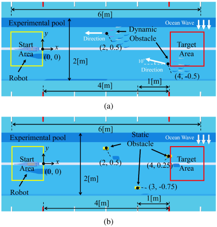
Fig. 4. Experimental environment for obstacle avoidance. (a) Dynamic obstacle avoidance. (b) Static obstacle avoidance.
The fundamental performance of the method was evaluated under five scenarios: wall-only (no obstacles), dynamic obstacles with and without ocean waves, and static obstacles with and without ocean wave. A comprehensive evaluation was conducted, including ablation studies with and without r-STDP learning, ocean wave disturbances, changes in PVC parameters, and comparisons between enclosed and open ocean environments. The testing was conducted 100 times and evaluated based on success rate (SR), coefficient of variation (CV), failure quality (FQ), mean steps to success (MSS), and failure (MSF).
4.2. Results with and Without Learning
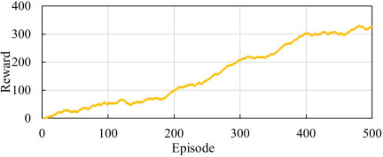
Fig. 5. Rewards for learning episode of the dynamic obstacle without ocean wave.
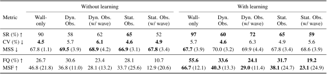
The relationship between episodes and rewards after learning for 500 episodes in a dynamic obstacle environment without ocean wave is shown in Fig. 5. Learning terminates when a predefined number of episodes is reached, or the reward variation satisfies the threshold. After each episode, the weights of the synaptic connections were updated using the r-STDP rule. Fig. 6 shows representative snapshots of the validation results for each scenario using the synaptic connection weights after learning. A performance comparison with and without learning of obstacle avoidance in each scenario is shown in Table 3. In this table, ↑ and ↓ indicate higher is better and lower is better, respectively. With learning, the wall-only (no obstacles) scenario achieved a 97\(\%\) SR in reaching the target area without colliding with walls. For dynamic obstacle avoidance, the robot reached the target area without collision at an SR of 60\(\%\) without ocean waves and 72\(\%\) with ocean waves. For the static obstacles, the target area was reached with an SR of 65\(\%\) without ocean waves and 59\(\%\) with ocean waves. These results demonstrate that the trained model achieved a higher SR than the model without learning. This proves that the proposed method successfully acquires basic obstacle avoidance behavior. The PVC-based SNN-CPG architecture achieved static and dynamic obstacle avoidance using only neural circuits. In highly critical safety scenarios, integrating high-level control as a path planning method into the proposed method is expected to improve the SR. The CV at success, with or without learning, showed stable performance with small variations. Stable avoidance performance without the presence of waves or static/dynamic obstacles indicates the capability to perform robust avoidance behaviors when integrated with path planning. The response to obstacle avoidance improved with learning. Hence, both the variation and MSS step counts increase, representing a trade-off relationship. Both FQ and MSF improved through learning. This indicates that the architecture can learn behaviors using only neural circuits. The relatively low FQ value indicates that the proposed method has learned the basic local avoidance behavior; however, its long-term planning capability remains insufficient.
4.3. Effect of PVC Parameter Variations
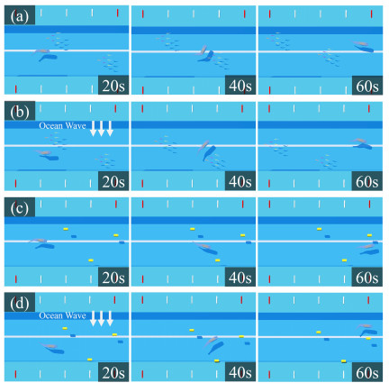
Fig. 6. Representative snapshots of experimental results. (a) Dynamic obstacle. (b) Dynamic obstacle with ocean wave. (c) Static obstacle. (d) Static obstacle with ocean wave.
Table 3. Performance comparison with and without r-STDP learning under different obstacle avoid scenarios. MSS and MSF is reported as mean (SD) in units of \(10^3\) steps.
The metrics for each scenario were evaluated to verify the effectiveness of the PVC direction preference in an experimental pool environment. Fig. 7 shows the relationship between PVC parameters variation and corresponding metrics. The SR tends to increase up to 30° as the preferred direction increases in Fig. 7(a). A positive correlation was observed between the CV and an increase in the preferred direction, as shown in Fig. 7(b). As the preferred direction increases, the sensitivity to stimuli from obstacles around the robot increases. Therefore, the SR increases to quickly detect obstacles that should be avoided and perform avoidance behaviors, leading to larger variance. The FQ value exhibits no significant change in response to variations in the preferred direction, as shown in Fig. 7(c). This implies that the failure patterns are limited by the shape of the robot and environment configuration. The narrow environment of the enclosed experimental pool is considered to be a limiting factor. Therefore, the PVC parameters need to be appropriately defined based on the SR and the quality of obstacle avoidance.
4.4. Performance Under Different Environmental Scenarios
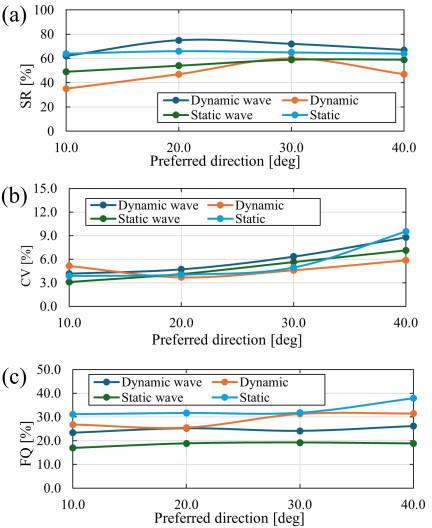
Fig. 7. Effect of PVC parameter variations on metric performance: (a) SR, (b) CV, and (c) FQ.
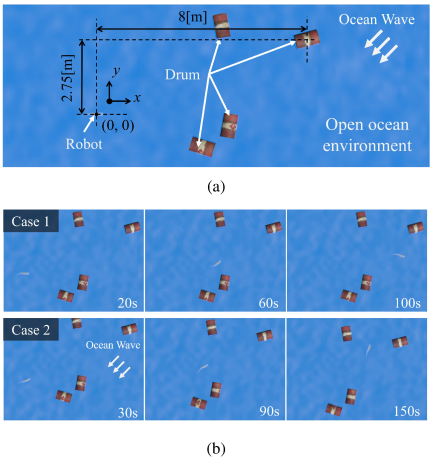
Fig. 8. Open ocean experiments. (a) Overview of open ocean. (b) Result of performance with and without ocean wave.
The effectiveness of the proposed method was evaluated through simulations assuming an open ocean environment. The system parameters for this scenario used default settings and trained weights. The results of the experiments conducted in open ocean environments with and without ocean waves are shown in Fig. 8. In the open ocean environment, an ocean wave with a stronger flow of 0.05 m/s in the diagonal flow direction was applied compared to the enclosed environment. In both case 1 (without ocean waves) and case 2 (with ocean waves), it was confirmed that the robot could proceed without colliding with the obstacles. The three-layer architecture can perform avoidance behaviors in unknown environments because of its various parameters and learning capabilities. It is also expected to be practical, based on its obstacle avoidance performance in simulated environments with ocean waves.
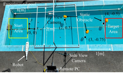
Fig. 9. Experimental outdoor environment.
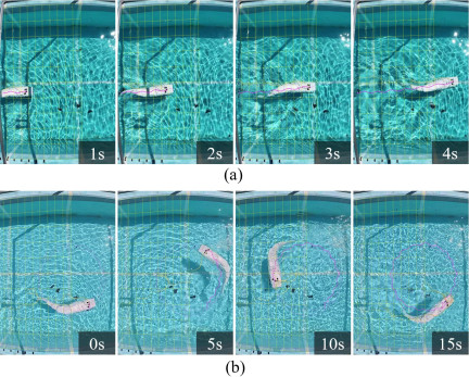
Fig. 10. Snapshots of the fundamental locomotion. (a) Forward motion, (b) yaw rotation.
5. Experiments in a Physical Environment
5.1. Results of the Fundamental Locomotion
To evaluate the proposed method, experiments are conducted on the fundamental locomotion of robots. Fig. 9 shows the experimental outdoor environment used for each evaluation of fundamental locomotion and obstacle avoidance. The onboard system of the robot executes the motor and sensor drivers to detect obstacles. On the remote PC, navigation commands are executed up to the sensory neurons, interneurons, and PVC motor neurons. For obstacle avoidance in the outdoor environment, the obstacles were placed in the same manner as those in the simulation environment. Fundamental locomotion was measured using a top-view camera mounted above an outdoor environment. The surge velocity was measured by varying the frequency of the forward motion from 0.6 Hz to 1.6 Hz in 0.2 Hz increments. The angular velocity was measured by varying the yaw rotation frequency in 0.2 Hz increments between 0.6 and 1.2 Hz. Measurements were conducted twice for each frequency, time-averaged, and then ensemble-averaged. Fig. 10 shows snapshots of the forward movement at 1.6 Hz and yaw rotation at 1.2 Hz, respectively. The variations in the surge and angular velocities of the yaw rotation with respect to frequency are shown in Fig. 11. As shown in Figs. 10(a) and 11(a), the surge velocity increased with higher frequencies, and achieved a maximum of 0.32 m/s. As shown in Figs. 10(b) and 11(b), the angular velocity of the yaw rotation reached a maximum of 0.41 rad/s. This indicates that swimming ability is required for both static and dynamic obstacle avoidance. In addition, fundamental studies of different environmental scenarios were conducted (Appendix A).
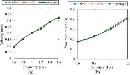
Fig. 11. Results of the fundamental locomotion. (a) Surge velocity, (b) yaw rotation.
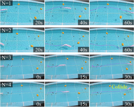
Fig. 12. Results of the obstacle avoidance.
5.2. Results of the Obstacle Avoidance
To verify the effectiveness of the proposed method, the static obstacle avoidance performance was evaluated using the trained weights. The preferred direction for the PVC was set to 30°, which achieved high SR values in each scenario, as shown in Fig. 7(a). The experiment was conducted four times as a part of an outdoor experiment. The results of the obstacle avoidance experiment are shown as a snapshot in Fig. 12. In the cases of \(N=1\) to \(N=3\), the robot was observed adjusting its locomotion to avoid static obstacles and walls as it approached them. The results of the experimental results demonstrated that the robot could reach the target area while avoiding obstacles. This substantiates the idea that stimuli from each sensory neuron adjust motor neurons via PVCs. When \(N=4\), the robot collides with the third static obstacle after avoiding the second static obstacle. This involves a variety of factors, including the detection of obstacles within the water and the velocity of the robot.
5.3. Limitations
The proposed method has the potential to achieve obstacle avoidance in unknown environments using only neural circuits, but it faces the following challenges:
-
The strength of the synaptic connections and the excitatory and inhibitory settings in the weight matrix require appropriate determination and learning based on the shape and velocity of the robot.
-
The proposed obstacle avoidance was performed at the neural circuit level; therefore, it is recommended that a high-level controller be integrated to ensure SR and stability.
Biologically feasible and robust behaviors can be expected through the incorporation of local and global path planners. Long-term memory enables the stability of long-term operational planning. The proposed vector-coding scheme is adaptable to different types of biomimetic robots.
6. Conclusions
An obstacle avoidance method using a PVC-based SNN-CPG architecture, inspired by locomotor neural circuits was proposed. This architecture consistently reproduces the neural circuit from the external stimuli to the motor neurons by adapting the PVC to the SNN-CPG structure. Obstacle avoidance skills can be acquired by learning the synaptic connection strengths using the r-STDP rule. This consistent architecture of the neural circuit enables the acquisition and learning of avoidance behaviors in unknown environments. To evaluate obstacle avoidance capability, experiments were conducted across five scenarios in a simulation environment. We conducted a comprehensive evaluation of ablation studies with and without learning, parameter effects, and experiments in different environments. Experiments were also conducted to verify the effectiveness of the obstacle avoidance capabilities in outdoor environments. The neural circuit alone exhibited fundamental obstacle avoidance capabilities in an unknown environment with static and dynamic obstacles and with or without ocean waves. These results indicate that the proposed three-layer architecture is capable of obstacle avoidance, and can adapt to unknown environments. The results demonstrated the ability to avoid obstacles in outdoor physical environments.
The novelty of this study is that obstacle avoidance was achieved using only reflexive movements, without relying on specific scenario environments or avoidance behavior models. Compared to previous studies, this study demonstrated that decoding using PVC and the three-layer SNN-CPG architecture performs the roles of reflexes, learning, and motor control within the architectural structure. By incorporating neural circuits into higher-level applications, it is expected to adapt to underwater robots with diverse shapes and numbers of joints and enable bio-inspired behaviors. In future works, we will investigate the neural circuits for dynamic obstacle avoidance in unknown environments with flowing seawater currents. To achieve robust avoidance behavior, each scenario requires an accurate selection of the preferred direction. The integration of neural circuits with path planning methods aims to achieve obstacle avoidance behavior that incorporates biological reflex mechanisms.
Appendix A. Aquarium Environment
Fundamental locomotion behaviors under different environmental scenarios were verified. The experiment was conducted in an aquarium environment, specifically focusing on yaw rotation. Fig. 13 shows the environment and yaw rotation performance at a frequency of 0.6 Hz. This robot was confirmed to be capable of moving in various environments, including freshwater and seawater. This additional experiment was necessary to evaluate the performance of the robot, both for use in different experiments and for learning purposes.
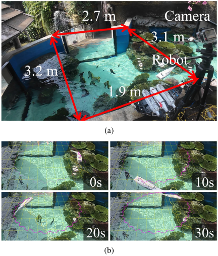
Fig. 13. Experiments in a aquarium environment. (a) Overview of the aquarium environment, (b) result of yaw rotation performance.
Acknowledgments
The authors would like to thank the Nakagawa Aquatic Park, Otawara, Tochigi, Japan, for their cooperation.
- [1] A. J. Ijspeert and M. A. Daley, “Integration of feedforward and feedback control in the neuromechanics of vertebrate locomotion: A review of experimental, simulation and robotic studies,” J. of Experimental Biology, Vol.226, No.15, Article No.jeb245784, 2023. https://doi.org/10.1242/jeb.245784
- [2] M. G. Sirota, G. V. Di Prisco, and R. Dubuc, “Stimulation of the mesencephalic locomotor region elicits controlled swimming in semi-intact lampreys,” European J. of Neuroscience, Vol.12, No.11, pp. 4081-4092, 2000. https://doi.org/10.1046/j.1460-9568.2000.00301.x
- [3] X. Zhang, Y. Cao, J. Huang, J. Liu, and Z.-Q. Zhang, “A systematic review of spiking neural networks for human-robot interaction in rehabilitative wearable robotics,” IEEE Trans. on Cognitive and Developmental Systems, Vol.8, No.1, pp. 6-21, 2026. https://doi.org/10.1109/TCDS.2025.3599432
- [4] M. Aitsam, S. Davies, and A. Di Nuovo, “Neuromorphic computing for interactive robotics: A systematic review,” IEEE Access, Vol.10, pp. 122261-122279, 2022. https://doi.org/10.1109/ACCESS.2022.3219440
- [5] J. Liu, H. Lu, Y. Luo, and S. Yang, “Spiking neural network-based multi-task autonomous learning for mobile robots,” Engineering Applications of Artificial Intelligence, Vol.104, Article No.104362, 2021. https://doi.org/10.1016/j.engappai.2021.104362
- [6] H. Lu, J. Liu, Y. Luo, Y. Hua, S. Qiu, and Y. Huang, “An autonomous learning mobile robot using biological reward modulate STDP,” Neurocomputing, Vol.458, pp. 308-318, 2021. https://doi.org/10.1016/j.neucom.2021.06.027
- [7] Z. Bing, C. Meschede, G. Chen, A. Knoll, and K. Huang, “Indirect and direct training of spiking neural networks for end-to-end control of a lane-keeping vehicle,” Neural Networks, Vol.121, pp. 21-36, 2020. https://doi.org/10.1016/j.neunet.2019.05.019
- [8] Z. Ali, L. Al-Amir, and A. Safa, “On the Importance of Neural Membrane Potential Leakage for LIDAR-based Robot Obstacle Avoidance using Spiking Neural Networks,” arXiv preprint, arXiv:2507.09538, 2025. https://doi.org/10.48550/arXiv.2507.09538
- [9] Y. Wang, B. Dong, Y. Zhang, Y. Zhou, H. Mei, Z. Wei, and X. Yang, “Event-enhanced multi-modal spiking neural network for dynamic obstacle avoidance,” Proc. of the 31st ACM Int. Conf. on Multimedia, pp. 3138-3148, 2023. https://doi.org/10.1145/3581783.3612147
- [10] M. S. Shim and P. Li, “Biologically inspired reinforcement learning for mobile robot collision avoidance,” 2017 Int. Joint Conf. on Neural Networks (IJCNN), pp. 3098-3105, 2017. https://doi.org/10.1109/IJCNN.2017.7966242
- [11] J. Chen, B. Yin, C. Wang, F. Xie, R. Du, and Y. Zhong, “Bioinspired closed-loop CPG-based control of a robot fish for obstacle avoidance and direction tracking,” J. of Bionic Engineering, Vol.18, No.1, pp. 171-183, 2021. https://doi.org/10.1007/s42235-021-0008-0
- [12] L. Zuo, M. Wang, Y. Gong, R. Wang, Q. Zhao, X. Zheng, and H. Gao, “SNN-CPG Hierarchical Control Enhanced Motion Performance of Robotic Fish Based on STDP,” Int. Conf. on Neural Computing for Advanced Applications, pp. 422-436, 2024. https://doi.org/10.1007/978-981-97-7001-4_30
- [13] M. Wang, Y. Zhang, and J. Yu, “An SNN-CPG hybrid locomotion control for biomimetic robotic fish,” J. of Intelligent & Robotic Systems, Vol.105, No.2, Article No.45, 2022. https://doi.org/10.1007/s10846-022-01664-7
- [14] I. Polykretis, M. Aanjaneya, and K. P. Michmizos, “Bioinspired Dynamic Control of Amphibious Articulated Creatures with Spiking Neural Networks,” Proc. of Graphics Interface 2023, 2022.
- [15] J. L. van Hemmen and A. B. Schwartz, “Population vector code: A geometric universal as actuator,” Biological Cybernetics, Vol.98, No.6, pp. 509-518, 2008. https://doi.org/10.1007/s00422-008-0215-3
- [16] R. Levi and J. M. Camhi, “Population vector coding by the giant interneurons of the cockroach,” J. of Neuroscience, Vol.20, No.10, pp. 3822-3829, 2000. https://doi.org/10.1523/JNEUROSCI.20-10-03822.2000
- [17] T. Asada, T. Oki, H. Furuhashi, K. Tabata, R. Miyagusuku, and K. Ozaki, “Performance Evaluation Using Sim2Real of a Robotic Dolphin with Multi-link Body Mechanism and CPG-based Controller,” IEEE Access, Vol.13, pp. 190304-190316, 2025. https://doi.org/10.1109/ACCESS.2025.3624365
- [18] T. I. Fossen, “Handbook of Marine Craft Hydrodynamics and Motion Control, 2nd ed.,” John Wiley & Sons, 2021.
- [19] H. Lamb, “Hydrodynamics,” Cambridge University Press, 1924.
- [20] X. Liao, C. Zhou, Q. Zou, J. Wang, and B. Lu, “Dynamic modeling and performance analysis for a wire-driven elastic robotic fish,” IEEE Robotics and Automation Letters, Vol.7, No.4, pp. 11174-11181, 2022. https://doi.org/10.1109/LRA.2022.3197911
- [21] H. Yang, Z. Yan, W. Zhang, Q. Gong, Y. Zhang, and L. Zhao, “Trajectory tracking with external disturbance of bionic underwater robot based on CPG and robust model predictive control,” Ocean Engineering, Vol.263, Article No.112215, 2022. https://doi.org/10.1016/j.oceaneng.2022.112215
- [22] M. Deger, M. Helias, C. Boucsein, and S. Rotter, “Statistical properties of superimposed stationary spike trains,” J. of Computational Neuroscience, Vol.32, No.3, pp. 443-463, 2012. https://doi.org/10.1007/s10827-011-0362-8
- [23] R. R. Buss and P. Drapeau, “Synaptic drive to motoneurons during fictive swimming in the developing zebrafish,” J. of Neurophysiology, Vol.86, No.1, pp. 197-210, 2001. https://doi.org/10.1152/jn.2001.86.1.197
- [24] E. M. Izhikevich, “Which model to use for cortical spiking neurons?,” IEEE Trans. on Neural Networks, Vol.15, No.5, pp. 1063-1070, 2004. https://doi.org/10.1109/TNN.2004.832719
- [25] J. Moran and R. Desimone, “Selective attention gates visual processing in the extrastriate cortex,” Science, Vol.229, No.4715, pp. 782-784, 1985. https://doi.org/10.1126/science.4023713
- [26] H. Bleckmann and R. Zelick, “Lateral line system of fish,” Integrative Zoology, Vol.4, No.1, pp. 13-25, 2009. https://doi.org/10.1111/j.1749-4877.2008.00131.x
- [27] J. Engelmann and H. Bleckmann, “Coding of lateral line stimuli in the goldfish midbrain in still and running water,” Zoology, Vol.107, No.2, pp. 135-151, 2004. https://doi.org/10.1016/j.zool.2004.04.001
- [28] E. Angelidis, E. Buchholz, J. Arreguit, A. Rougé, T. Stewart, A. von Arnim, A. Knoll, and A. Ijspeert, “A spiking central pattern generator for the control of a simulated lamprey robot running on SpiNNaker and Loihi neuromorphic boards,” Neuromorphic Computing and Engineering, Vol.1, No.1, Article No.014005, 2021. https://doi.org/10.1088/2634-4386/ac1b76
- [29] R. V. Florian, “Reinforcement learning through modulation of spike-timing-dependent synaptic plasticity,” Neural Computation, Vol.19, No.6, pp. 1468-1502, 2007. https://doi.org/10.1162/neco.2007.19.6.1468
- [30] M. Mozafari, S. R. Kheradpisheh, T. Masquelier, A. Nowzari-Dalini, and M. Ganjtabesh, “First-spike-based visual categorization using reward-modulated STDP,” IEEE Trans. on Neural Networks and Learning Systems, Vol.29, No.12, pp. 6178-6190, 2018. https://doi.org/10.1109/TNNLS.2018.2826721
- [31] M. Akl, Y. Sandamirskaya, D. Ergene, F. Walter, and A. Knoll, “Fine-tuning deep reinforcement learning policies with r-STDP for domain adaptation,” Proc. of the Int. Conf. on Neuromorphic Systems 2022, Article No.14, 2022. https://doi.org/10.1145/3546790.3546804
This article is published under a Creative Commons Attribution-NoDerivatives 4.0 Internationa License.