Paper:
Orchard Navigation of UGVs Using UAV-LiDAR-Based Semantic Costmap
Soki Nishiwaki, Shuhei Yoshida, and Takanori Emaru
Faculty and Graduate School of Engineering, Hokkaido University
Kita 13, Nishi 8, Kita-ku, Sapporo, Hokkaido 060-8628, Japan

This study proposes a costmap generation method for orchard navigation that integrates both semantic and geometric information from point clouds acquired using unmanned aerial vehicle (UAV)-based light detection and ranging (LiDAR). Conventional approaches often rely on aerial imagery, which cannot capture the internal structures of tree crowns, or on ground-based mapping, which is inefficient and typically limited to height-based costmaps. In this study, orchard-scale three-dimensional point clouds were acquired using UAV-LiDAR, and RandLA-Net was applied for semantic segmentation to classify tree trunks, crowns, and ground. Based on this classification, we constructed a semantic costmap that incorporates obstacle height and shape and integrated it into the Navigation2 framework for unmanned ground vehicle (UGV) navigation. Simulation experiments (20 trials) achieved an 85% success rate, significantly higher than that of conventional methods (60%–65%). Furthermore, field experiments (15 trials) achieved a 93% success rate, demonstrating safe and efficient path planning even in densely canopied environments.
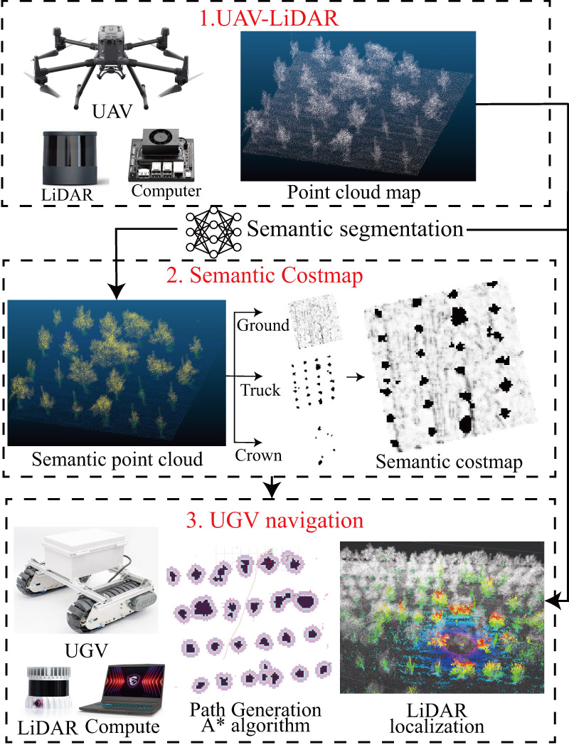
Orchard navigation pipeline
1. Introduction
Agriculture is currently facing two major global challenges: increasing food demand driven by population growth and a persistent labor shortage. According to the Food and Agriculture Organization, global primary crop production reached approximately 9.9 billion tons in 2023, with fruit production accounting for approximately 10\(\%\) of the total, representing a major agricultural sector a. Despite its importance, fruit production remains highly labor-intensive compared with large-scale grain production, where automated operations have been widely adopted. Core operations such as pruning, thinning, pest control, weeding, and harvesting still rely heavily on manual labor, resulting in a substantial economic burden. Reports from the United States Department of Agriculture Economic Research Service indicate that labor costs account for up to 38% of total production costs in fruit farming, posing a serious threat to long-term sustainability b. In addition to these global trends, the situation in Japan is particularly severe. Over the decade from 2005 to 2015, the average age of orchard operators increased from 61 to 77 years, highlighting rapid workforce aging c. This critical labor shortage, coupled with a lack of successors, has led to widespread orchard abandonment and a continuous decline in cultivated areas. Moreover, many Japanese orchards adopt traditional cultivation systems with complex tree geometries to maximize land-use efficiency. While effective for improving fruit quality, these systems significantly hinder the deployment of medium- and large-scale agricultural machinery.
Therefore, the development of compact robotic systems capable of autonomous operation and high maneuverability in narrow, semi-structured orchard environments is essential not only for labor reduction but also for sustaining fruit production systems 1.
This study focuses on supporting autonomous navigation for small-scale robotic platforms performing tasks such as fruit transportation and undergrowth mowing. These tasks require robots to operate while navigating between tree rows, making stable navigation and reliable self-localization indispensable.
In the orchards considered in this study, aisle widths are typically approximately 3 m, with narrow sections as small as 1 m. For a robot with a width of 0.5 m to traverse a 1 m aisle safely, the lateral deviation of the robot’s center from the aisle center must be maintained below 0.25 m. In this study, a goal tolerance of 0.5 m is adopted as a global criterion for goal-reaching evaluation to assess navigation performance without additional post-arrival alignment (e.g., corrective back-and-forth motions). However, this tolerance is used only for global-level performance evaluation and goal-reaching determination, and does not represent the allowable lateral deviation in the narrowest aisle. Safety in constrained regions is ensured through geometric constraints and LiDAR-based local obstacle avoidance.
Furthermore, safe navigation under such constraints requires path planning that explicitly accounts for obstacle distribution and spatial structure within tree rows. In particular, when robots operates beneath the canopy, they must avoid not only trunks but also branches and foliage.
Autonomous navigation has advanced considerably in structured environments, particularly in domains such as self-driving vehicles and logistics robots. These environments, characterized by designed features, such as lanes, walls, shelves, and corridors, offer regular and predictable layouts. As a result, simultaneous localization and mapping (SLAM) and path planning are more robust, and many practical systems have been realized 2.
In contrast, autonomous navigation in semi-structured environments such as orchards and farms remains a challenge 3. Although features such as tree rows and farm roads provide a degree of regularity, these environments are not fully organized due to overhanging branches, uneven ground, and other irregularities.
Consequently, navigation in orchards requires both precise map generation and safe path planning; however, existing approaches remain limited. For map generation, ground-based measurements using UGVs provide high accuracy but require significant time to cover large areas. In contrast, aerial measurements using UAVs equipped with image sensors—sensors, the most common approach—are efficient; however, they capture only surface information on tree crowns and fail to represent internal structures. In path planning, grid-based costmaps generally incorporate trunk positions but omit branches and foliage, leaving safety concerns unresolved. This limitation is particularly critical for small-scale robotic platforms, such as those used for fruit transport or weeding, which operate beneath the canopy and traverse crop rows. Therefore, the development of a costmap generation method that explicitly considers both trunks and crowns is essential for enabling the safe operation of such robotic platforms 4.
In our previous study, we developed a method for orchard mapping using UAV-LiDAR-based SLAM, enabling the acquisition of detailed three-dimensional (3D) structures at a low cost 5. In this study, we extend this work by constructing a costmap based on UAV-LiDAR point clouds and applying it to UGV localization and path planning. The proposed pipeline is illustrated in Fig. 1.
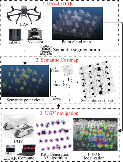
Fig. 1. Overview of the proposed pipeline for orchard navigation, including UAV-LiDAR mapping (Section 3.1), semantic segmentation (Section 3.2), costmap generation (Section 3.3), and UGV localization and path planning (Sections 3.5 and 3.6).
The effectiveness of the proposed approach was verified through field experiments in an actual orchard, where a 3D map generated using UAV-LiDAR was employed for UGV localization and path planning. We evaluated our method against two baselines: projection of the point cloud onto the \(XY\)-plane to simulate aerial imagery and an approach that considers only trunk point clouds. As a result, the proposed method successfully balances safety and efficiency in UGV path planning.
The main contributions of this study are as follows:
-
A novel costmap generation method is proposed that integrates spatial information from both trunks and crowns by introducing semantic labels into UAV-LiDAR point clouds. This approach explicitly represents the under-canopy space, which has been overlooked in conventional trunk-based or ground-projection costmaps.
-
A complete pipeline for UGV localization using pre-acquired UAV point clouds is developed and validated in real orchard environments, demonstrating both safety and efficiency.
3. Materials and Method
3.1. UAV 3D Mapping
In this study, we generated 3D orchard maps using the UAV-LiDAR system shown in Fig. 1(a), which consists of a DJI Matrice 300 RTK equipped with a Hesai QT-128 LiDAR sensor. For UAV flight control, the DJI Pilot application was used, and an NVIDIA Jetson Nano was employed for LiDAR data acquisition. The flight conditions were set to a speed of 2 m/s and an altitude of 10 m to ensure that the LiDAR scanning range sufficiently covered the entire field. The flight path was executed autonomously based on predefined waypoints, enabling efficient scanning of the entire field. These flight conditions were determined by balancing point-cloud density and flight efficiency. An altitude of 10 m was selected to ensure complete acquisition of both crown and trunk structures.
The collected data were subsequently processed using a LiDAR-SLAM algorithm 5 to generate a 3D point cloud map.
Table 1. Classification performance of RandLA-Net on the orchard dataset. Accuracy and IoU are reported for all classes (ground, trunk, crown).

3.2. Semantic-Segmentation of UAV-LiDAR Point Clouds
The 3D point cloud obtained from UAV-LiDAR was classified into three semantic categories: ground, trunk (including support poles), and crown. The trunk class includes both trunk points and supporting poles of the trees. For semantic segmentation, RandLA-Net 32,33 was employed because it is well suited for the efficient processing of large-scale point clouds using random sampling. A model pre-trained on the DALES dataset 34, an airborne LiDAR dataset, was used as the base model. For fine-tuning, an orchard dataset collected over a three-year period (2022–2024) was used. The original training set consisted of 501 annotated point cloud instances. To enhance model robustness and prevent overfitting, data augmentation was performed by randomly tilting the point clouds within a range of 0°–2° and rotating them by 90°, 180°, and 270° around the \(z\)-axis, resulting in a total of 1,935 training instances. Training was conducted on an NVIDIA RTX 4090 GPU with a mini-batch size of 12, an initial learning rate of 0.01, and a total of 300 epochs.
As shown in Table 1, the ground and crown classes were segmented with high accuracy (0.996 and 0.963, respectively) and high intersection over union (IoU) (0.993 and 0.947, respectively). In contrast, the trunk class achieved a moderate accuracy of 0.719 but a relatively low IoU of 0.445. This discrepancy indicates that although most trunk points were correctly classified in proportion to the entire dataset, a considerable number of trunk points were either missed (false negatives) or confused with the crown points (false positives). Because the accuracy reflects the ratio of correctly classified points over the entire dataset, it remains relatively high for the trunk class, which is a minority class. However, the IoU is more sensitive to class-specific errors; therefore, the trunk class exhibited a lower value. This quantitative result confirms that boundary misclassifications between trunks and crowns are the main factors degrading trunk metrics. As illustrated in Fig. 2, typical errors include low-lying crowns predicted as trunks and upper poles predicted as crowns. In both cases, the affected regions are still mapped as obstacles (either trunk or crown) on the \(XY\)-plane grid, indicating that the correctness of the costmap generation is preserved. A truly critical case would be the misclassification of ground points as trunks or crowns, which would cause traversable areas to be erroneously treated as obstacles. However, such cases were not observed in our experiments. Therefore, the impact of these segmentation errors on the UGV navigation was minimal.
3.3. Semantic Costmap Generation
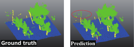
Fig. 2. Example results of semantic segmentation using RandLA-Net. Left: ground truth; right: prediction. Colors: ground (blue), trunk (yellow), and crown (green). Typical misclassifications include low crowns near the ground labeled as trunks and upper trunks labeled as crowns.
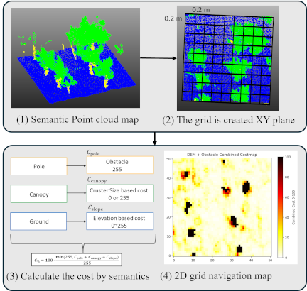
Fig. 3. Overview of semantic costmap generation. Costs are assigned to each cell based on semantic labels (e.g., ground, trunk, crown), and the resulting costmap is used for UGV navigation.
An overview of the proposed semantic costmap generation process is presented in Fig. 3. A two-dimensional grid covering the entire field was defined with a resolution of \(0.2~\mathrm{m}\), selected based on the approximate robot size (about \(0.5~\mathrm{m}\)) to provide spatial granularity corresponding to roughly half of the robot’s footprint. Each cell \((x,y)\) was assigned an initial cost based on the semantic classification of the UAV-LiDAR point cloud (ground, trunk, and crown).
The final normalized cost \(C_{\%}\) is defined as follows:
3.3.1. Trunk
The trunk point clouds were first filtered to remove points above a height of \(0.7~\mathrm{m}\) relative to the ground, considering the physical height of the UGV, to focus on the lower structures that pose a direct collision risk. The trunk point clouds were clustered using density-based spatial clustering of applications with noise (DBSCAN), and the centroid of each cluster \(P_c\) was computed as \(\mathbf{p}_c = (x_c, y_c)\). The minimum distance between clusters was defined as follows:
3.3.2. Crown
For crown point clouds, points were first filtered based on height above the ground, satisfying \(\Delta z = z_{\mathrm{crown}} - z_{\mathrm{ground}} \le \tau_z = 1.0~\mathrm{m}\). Considering the physical height of the UGV, points with \(\Delta z \le 0.7~\mathrm{m}\) were treated as obstacles, as the corresponding cells were assigned the maximum cost (255). Points with \(0.7~\mathrm{m} < \Delta z \le 1.0~\mathrm{m}\) were retained for clustering. These retained points were clustered using DBSCAN \((\varepsilon = 0.2~\mathrm{m},\, \text{min\_samples}=5)\), and the set of noise-removed crown clusters was denoted by \(\{C_c\}_{k=1}^K\). For each cluster \(C_c\), the points were projected onto the \(XY\)-plane, and the spatial extent was defined using Eq. \(\eqref{eq:cluster_extent}\):
3.3.3. Slope (Ground)
The local slope angle was defined as in Eq. \(\eqref{eq:slope_angle}\):
3.3.4. Merged Costmap
The final merged costmap \(C\) was obtained by summing the obstacle costs \(C_{\mathrm{trunk}}\), \(C_{\mathrm{crown}}\), and the slope cost \(C_{\mathrm{slope}}\), and clipping the resulting value to an upper bound \(255\).
To ensure compatibility with Navigation2 35 in ROS 2 [36, d], the final costmap \(C_{\mathrm{\%}}\) was normalized to a scale of \([0,100]\).
3.4. UGV Hardware System
The UGV used in this study was a CuboRex Cugo V3i, which employs a crawler-type drive system. This configuration provides high mobility in complex orchard environments, including rough terrain, muddy ground, and sloped areas.
An Ouster OS1-128 LiDAR sensor was mounted on the vehicle as the primary sensor. The OS1-128 is a 128-channel 3D LiDAR with a maximum measurement range of approximately 120 m and a field of view covering 360° horizontally and 45° vertically. It achieves centimeter-level measurement accuracy and can generate high-density point clouds at approximately 2.5 million points per second. In addition, its multi-return capability and intensity information are effective for distinguishing between different targets such as tree trunks, branches, foliage, and the ground surface.
For computation, a laptop PC (Core i7-13620H, 10 cores [6P+4E], 16 threads, NVIDIA RTX 4060 Laptop GPU) was used. The LiDAR-SLAM and path-planning algorithms were executed in an Ubuntu 22.04 LTS environment with ROS 2.
3.5. UGV Localization Using a 3D Map
For UGV localization, the lidarslam_ros2 package e for ROS 2 was used. This package uses a scan-matching method based on the normal distributions transform (NDT), which enables high-accuracy pose estimation by aligning real-time LiDAR scans with a prior 3D map. For initial pose estimation, odometry (odom) information from the encoders mounted on the Cugo V3i was utilized. In this study, a 3D point cloud map of the orchard, obtained using the UAV-LiDAR system on October 30, 2024, was used as a prior map. This prior map contains dense structural information about the orchard, such as trunks and crowns, and serves as a reference for NDT scan matching.
3.6. UGV Navigation
For UGV navigation, the Navigation2 package f of ROS 2 was employed. Navigation2 provides functions such as global path planning (planner server), local path following and obstacle avoidance (controller server), and integrates the proposed costmap generation method. The coordinate system followed the TF tree of map-odom-base_link. Obstacle information obtained from sensors was integrated into both global and local costmaps and reflected in path generation.
In this study, the semantic costmap generated from the UAV-LiDAR point cloud was integrated into Navigation2 as the global costmap. Furthermore, during navigation, dynamic obstacle detection from the Ouster LiDAR was incorporated into the local costmap. By combining a static map with dynamic sensor information, safe and efficient navigation was achieved.
The global path was generated using the standard Navigation2 planner based on the A\(^{*}\) algorithm g, while local path following was performed using the dynamic window approach (DWB) controller h. The DWB controller generates velocity samples considering the robot’s kinematics and determines optimal control inputs based on both path tracking accuracy and obstacle avoidance capability.
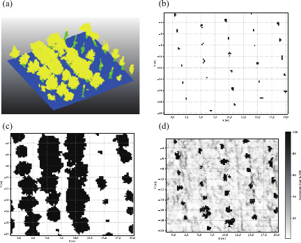
Fig. 4. Example of the costmaps: (a) orchard point cloud map, (b) Baseline 1 costmap, (c) Baseline 2 costmap, and (d) proposed costmap. In the proposed costmap, additional costs are assigned around tree trunks by accounting for obstructive canopy elements (e.g., leaves and branches), and ground cells are weighted according to terrain slope.
3.7. Experiment Setup
To evaluate the performance of our proposed pipeline against conventional approaches, UGV navigation experiments were conducted using three different types of costmaps.
-
Proposed: A semantic costmap explicitly representing trunks, crowns, and ground.
-
Baseline 1: A costmap constructed from point cloud height and density thresholds 25. Cells were regarded as obstacles when the point cloud density within a specified height range exceeded predefined thresholds, thereby producing a height and density based costmap.
-
Baseline 2: A costmap generated by projecting the point cloud onto the \(XY\)-plane to simulate information equivalent to UAV aerial imagery 23.
A comparison of these methods is presented in Fig. 4. To generate the costmaps for Baseline 1 and Baseline 2, ground points classified by semantic segmentation were removed. For Baseline 1, a height threshold of 0.7 m was applied, and following the method of Zhenyu et al. 25, cells containing more than three points within the height range of 0.3–0.5 m were treated as obstacles. For Baseline 2, the point cloud was projected onto the \(XY\)-plane, and cells containing points were defined as obstacle regions. The resulting projection was interpreted as aerial imagery.
For each method, the following metrics were evaluated.
-
Goal-reaching rate (goal-reaching/failure)
-
Navigation time (time from start to goal achievement [s])
A tolerance of 50 cm was set as the criterion for goal achievement, considering the approximate footprint of the robot. The robot was considered to have reached the goal when it arrived within this range of the target position.
4. Experiments and Results
4.1. Simulation Experiment Results
In this section, the navigation performance based on the three types of costmaps is evaluated in a simulation environment using the Gazebo software. The simulation environment, covering an area of approximately \(140 \times 130\) m, was constructed from point cloud data acquired in an apple orchard in Hokkaido on October 30, 2024, and it served as a virtual platform for reproducing and evaluating UGV navigation.
The experiments were conducted with 20 trials in total: scenarios 1–10 involved short-distance paths of approximately 10 m, while scenarios 11–20 consisted of long-distance paths of approximately 50 m that traversed approximately 10 crop rows. The results are summarized in Table 2. Baseline 1, Baseline 2, and the proposed method succeeded in 12, 13, and 17 of 20 trials, respectively.


Table 3 lists the travel times of the proposed method and its differences from Baselines 1 and 2. In scenarios 1–10, the proposed method was on average \(+\)6.102 s slower than Baseline 2, whereas it achieved shorter goal-reaching times in all seven comparable trials relative to Baseline 1. This is because Baseline 1 considers only trunks, allowing shorter paths to be generated. In longer scenarios (11–20), only three failures were observed with the proposed method, whereas eight and seven failures were recorded with Baselines 1 and 2, respectively. This outcome can be attributed to the fact that the proposed method incorporates not only trunks but also canopies (branches and foliage) into the costmap. Therefore, narrow inter-row passages and insufficient clearance beneath the crown are assigned high costs and avoided in advance.
In terms of failure cases, collisions were observed when saplings were not represented in the costmap generated at a resolution of 0.2 m and when insufficient LiDAR points were acquired to detect obstacles reliably. The results of scenario 15, in which a large difference in travel time was observed between the proposed method and Baseline 2, are shown in Fig. 5. In this scenario, Baseline 2 recognized the canopy as an obstacle and therefore selected a significantly detoured path. Furthermore, scenario 17 corresponds to the case in which only Baseline 2 successfully reaches the goal as a result of selecting such a detoured path.
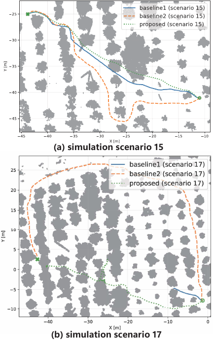
Fig. 5. UGV trajectories in simulation scenarios 15 and 17: (a) successful navigation example along a long-distance path, and (b) a long-distance path where only Baseline 2 successfully reached the goal.
4.2. Real-World Experimental Result
Field experiments were conducted on August 22, 2025, in an apple orchard in Hokkaido. Owing to time constraints, only short paths of approximately 10 m that traversed the crop rows were tested. For each costmap, 15 trials were conducted. In an orchard environment, fallen apples are present on the ground surfaces in certain areas. When a vehicle passes over fallen fruits, changes in wheel contact with the ground occasionally cause temporary disturbances in vehicle posture and heading. To prevent such effects from influencing the evaluation of the localization and navigation performance, fallen apples along the planned paths were removed in advance in all experimental trials.
An example of the experimental scenario is shown in Fig. 6. Scenarios 1–5 correspond to areas where the trees are still young and the crowns are not densely developed, whereas scenarios 6–15 correspond to areas with dense crowns and overhanging branches.
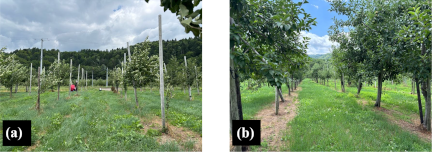
Fig. 6. Representative experimental scenarios: (a) scenarios 1–5 and (b) scenarios 6–15.


The goal-reaching rates of the experiments are summarized in Table 4, and the detailed results are presented in Table 5. Baselines 1 and 2 succeeded in 11 and 9 of 15 trials, respectively, whereas the proposed method succeeded in 14 of 15 trials. In scenarios 1–5, all three methods were successful in each trial. This indicates that, in environments where the trees are young and crowns are sparse, each method can work effectively. By contrast, in scenarios 6–15, the proposed method succeeded nine times, Baseline 1 succeeded seven times, and Baseline 2 succeeded only four times. The navigation trajectories of representative scenarios 1, 8, and 15 from an overhead perspective are illustrated in Fig. 7.
In scenario 1 (Fig. 7(a)), all three methods succeeded, and Baseline 1 reached the goal via the shortest path. This is because Baseline 1 does not account for the crowns, allowing it to generate the shortest route. In contrast, Baseline 2 and the proposed method treat regions containing crowns as obstacles, resulting in fewer direct routes.
In scenario 8 (Fig. 7(b)), Baseline 2 could not move from the start. In the Baseline 2 costmap, a large number of cells in densely clustered crown regions were recognized as obstacles, preventing the UGV from finding a traversable path, as shown in Fig. 8. In contrast, the costmaps of Baseline 1 and the proposed method allowed paths under the crowns where the UGV could pass, enabling both methods to successfully reach the goal.
In scenario 15 (Fig. 7(c)), Baseline 1 planned a more detoured route than the other methods, as it selected a path through regions where crowns did not overlap. For the Baseline 2 method, branches along the route acted as obstacles. Although the robot attempted to avoid them, it eventually failed to reach the goal. In contrast, the proposed method successfully reached the goal by generating a path based on a costmap that explicitly accounts for branches as show in Fig. 9.
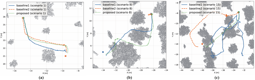
Fig. 7. UGV trajectories for scenarios 1, 8, 15 : (a) scenario 1, (b) scenario 8, and (c) scenario 15.
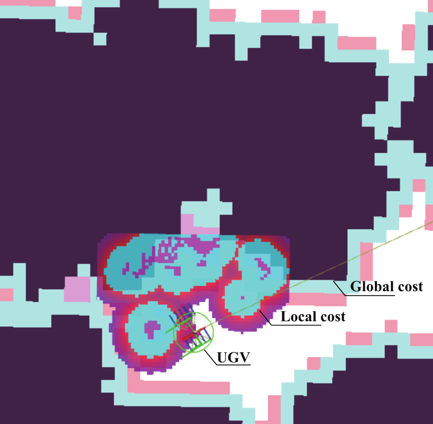
Fig. 8. Baseline 2 costmap in scenario 8, with the local costmap superimposed, showing the failure to generate a traversable path.
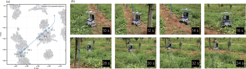
Fig. 9. UGV navigation in scenario 15: (a) navigation trajectory and (b) snapshots illustrating the navigation process at different time steps.
5. Discussion
Although the number of trials in this study was relatively modest (20 simulation runs and 15 field experiments), it is comparable to or exceeds those reported in related agricultural robotics studies 23,25,4. Importantly, the experiments covered diverse orchard layouts and canopy densities, and confidence intervals were reported in addition to the observed goal-reaching rates. Therefore, the evaluation is considered sufficient to demonstrate the effectiveness and robustness of the proposed method. However, larger-scale validation remains an important direction for future work.
In terms of the goal-reaching rate, the proposed method consistently outperformed the baseline methods in both simulations and real-world experiments. In simulation, the proposed method achieved an 85.0% goal-reaching rate (95% CI: 64.0–94.8), compared with 60.0% (38.7–78.1) for Baseline 1 and 65.0% (43.3–81.9) for Baseline 2. In the real-world experiments, the goal-reaching rate of the proposed method was 93.3% (70.2–98.8), compared with 73.3% (48.1–89.1) and 60.0% (35.7–80.2) for Baseline 1 and Baseline 2, respectively. The odds ratios were consistently greater than 1 across all comparisons, indicating a favorable trend toward the proposed method (e.g., \(\mathrm{OR} = 9.33\) vs. Baseline 2 in the real-world). However, the confidence intervals were wide and, in several cases, included one, reflecting the limited number of trials and the associated uncertainty. These results indicate that, although statistical significance at the 5% level cannot be established, the proposed method demonstrates a consistent performance advantage in terms of navigation reliability.
When considering only successful trials, the differences in travel times among the methods were less pronounced. Although variations in travel time are largely attributable to differences in path length, orchard environments often require local avoidance behaviors, such as in-place rotations, temporary stops, and re-planning. These behaviors can increase the total travel time without substantially affecting the overall path length. Therefore, travel time was employed as an evaluation metric to account for both global path characteristics and local navigation performance. In simulation, the proposed method showed a small reduction in travel time relative to Baseline 1 (mean difference: \(-8.0\) s, Cohen’s \(d=-0.37\)), while a larger numerical reduction was observed relative to Baseline 2 (\(-24.0\) s, \(d=-0.81\)). Similarly, in the real-world experiments, the proposed method tended to yield shorter travel times than both baselines (\(-5.8\) s vs. Baseline 1 and \(-3.8\) s vs. Baseline 2), with small effect sizes (\(d \approx -0.18\) to \(-0.31\)). However, the confidence intervals were wide and included zero, indicating that the differences in travel time were not statistically significant.
Overall, these findings suggest that the primary strength of the proposed method lies in its reliability and robustness, as evidenced by the consistently higher goal-reaching rates, rather than in achieving substantial reductions in travel time. The effect sizes indicated a tendency toward faster navigation, particularly compared with Baseline 2; however, additional experiments with larger sample sizes and greater scenario diversity are required to confirm these trends with statistical confidence. From a practical standpoint, ensuring successful task completion is more critical than marginal differences in travel time, especially in real-world agricultural robotics applications, where navigation failures can incur substantial operational costs. In both the simulation and real-world experiments, cases in which the UGV failed to reach the goal were observed. These failures were primarily caused by collisions with small-scale obstacles such as young saplings and thin supports scattered throughout the orchard.
The semantic costmap used in this study was configured with a grid resolution of 0.2 m to balance computational efficiency with navigation performance. At this resolution, thin crops and saplings with diameters of only a few centimeters are not explicitly projected onto the map, owing to grid discretization (quantization) effects. Furthermore, because these objects have small surface areas, the number of reflection points captured by the LiDAR sensor is extremely sparse. Consequently, there were instances in which such objects were not recognized as obstacles, leading to collisions (Fig. 10).
As shown in Table 3, there were scenarios in which only Baseline 2 succeeded, whereas the proposed method failed. This suggests that, although the proposed method effectively leverages major structures (e.g., trunks and rows) for navigation, it still faces limitations in local detection and avoidance capabilities for objects with low spatial occupancy.
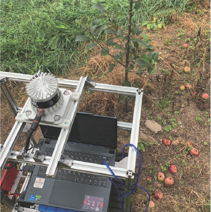
Fig. 10. Collision incident in real-world scenario 11, caused by failure to detect a thin tree due to sparse LiDAR point returns.
To address obstacles with difficult-to-capture geometries and further enhance robustness, it would be effective to expand the system toward a more integrated recognition framework. However, such a framework should not rely solely on LiDAR-based geometric data. Integrating additional sensing modalities, such as vision-based recognition, can improve the detection of minute obstacles. By incorporating semantic information alongside geometric features, it is possible to identify small or thin objects even when the point cloud data are sparse. Future work will focus on enabling safer and more precise navigation in complex agricultural environments by integrating diverse sensor information to improve obstacle detection.
While this study presents a proof-of-concept system for localization and navigation, the robustness to lateral deviations caused by ground disturbances (e.g., fallen objects) and vehicle vibrations remains a practical challenge for real-world deployment. An important next step is to quantitatively evaluate the vibration induced deviations under field conditions and derive specifications for the allowable lateral deviation required for safe and stable navigation. Future work should focus on achieving safer and more accurate navigation for real-world deployment through multi-modal sensing and improved motion control.
6. Conclusion
This study presents a novel costmap generation method that integrates spatial information from both trunks and crowns by incorporating semantic labels into 3D UAV-LiDAR point clouds. Unlike conventional height-based or aerial-imagery-based costmaps, the proposed approach explicitly represents under-canopy space, which is critical for safe navigation in orchards. Furthermore, the proposed method was implemented as a complete pipeline for UGV localization and path planning using a prior UAV-LiDAR map, and its effectiveness was validated through comparative experiments against two baseline methods. Both simulation and real-world experiments demonstrated that the proposed method consistently achieved higher success rates than the baselines, while maintaining comparable or shorter travel times. These results indicate that the primary strength of the proposed approach lies in its reliability and safety, enabling successful goal attainment even in narrow under-canopy spaces. The experiments demonstrate the practical advantage of explicitly modeling traversable space beneath the canopy, which has been overlooked in conventional approaches. Future work will focus on larger-scale validation across diverse orchard conditions and on further enhancing the adaptability of the proposed pipeline to different crop environments.
Acknowledgments
This work was supported by JST SPRING (Grant Number JPMJSP2119), the Azbil Yamatake Foundation, and JSPS KAKENHI (Grant Number 24K07413).
- [1] A. Jiang and T. Ahamed, “Navigation of an autonomous spraying robot for orchard operations using lidar for tree trunk detection,” Sensors, Vol.23, No.10, Article No.4808, 2023. https://doi.org/10.3390/s23104808
- [2] E. Yurtsever, J. Lambert, A. Carballo, and K. Takeda, “A survey of autonomous driving: Common practices and emerging technologies,” IEEE Access, Vol.8, pp. 58443-58469, 2020. https://doi.org/10.1109/ACCESS.2020.2983149
- [3] X. Li and Q. Qiu, “Autonomous navigation for orchard mobile robots: A rough review,” 2021 36th Youth Academic Annual Conf. of Chinese Association of Automation (YAC), pp. 552-557, 2021. https://doi.org/10.1109/YAC53711.2021.9486486
- [4] L. Ye, F. Wu, X. Zou, and J. Li, “Path planning for mobile robots in unstructured orchard environments: An improved kinematically constrained bi-directional RRT approach,” Computers and Electronics in Agriculture, Vol.215, Article No.108453, 2023. https://doi.org/10.1016/j.compag.2023.108453
- [5] S. Nishiwaki, H. Kondo, S. Yoshida, and T. Emaru, “Proposal of UAV-SLAM-based 3D point cloud map generation method for orchards measurements,” J. Robot. Mechatron., Vol.36, No.5, pp. 1001-1009, 2024. https://doi.org/10.20965/jrm.2024.p1001
- [6] H. Li, K. Huang, Y. Sun, X. Lei, Q. Yuan, J. Zhang, and X. Lv, “An autonomous navigation method for orchard mobile robots based on octree 3D point cloud optimization,” Frontiers in Plant Science, Vol.15, Article No.1510683, 2025. https://doi.org/10.3389/fpls.2024.1510683
- [7] X. Yao, Y. Bai, B. Zhang, D. Xu, G. Cao, and Y. Bian, “Autonomous navigation and adaptive path planning in dynamic greenhouse environments utilizing improved LeGO-LOAM and openplanner algorithms,” J. of Field Robotics, Vol.41, No.7, pp. 2427-2440, 2024. https://doi.org/10.1002/rob.22315
- [8] G. Cao, B. Zhang, Y. Li, Z. Wang, Z. Diao, Q. Zhu, and Z. Liang, “Environmental mapping and path planning for robots in orchard based on traversability analysis, improved LeGO-LOAM and RRT* algorithms,” Computers and Electronics in Agriculture, Vol.230, Article No.109889, 2025. https://doi.org/10.1016/j.compag.2024.109889
- [9] S. Pan, Y. Hu, A. Ohya, and A. Yorozu, “LiDAR mapping using point cloud segmentation by intensity calibration for localization in seasonal changing environment,” Smart Agricultural Technology, Vol.11, Article No.100970, 2025. https://doi.org/10.1016/j.atech.2025.100970
- [10] T. Lowe, P. Moghadam, E. Edwards, and J. Williams, “Canopy density estimation in perennial horticulture crops using 3D spinning lidar SLAM,” J. of Field Robotics, Vol.38, No.4, pp. 598-618, 2021. https://doi.org/10.1002/rob.22006
- [11] Y. Wang, Z. Zhang, W. Jia, M. Ou, X. Dong, and S. Dai, “A review of environmental sensing technologies for targeted spraying in orchards,” Horticulturae, Vol.11, No.5, Article No.551, 2025. https://doi.org/10.3390/horticulturae11050551
- [12] T. Shan and B. Englot, “LeGO-LOAM: Lightweight and ground-optimized lidar odometry and mapping on variable terrain,” 2018 IEEE/RSJ Int. Conf. on Intelligent Robots and Systems (IROS), pp. 4758-4765, 2018. https://doi.org/10.1109/IROS.2018.8594299
- [13] T. Shan, B. Englot, D. Meyers, W. Wang, C. Ratti, and D. Rus, “LIO-SAM: Tightly-coupled lidar inertial odometry via smoothing and mapping,” 2020 IEEE/RSJ Int. Conf. on Intelligent Robots and Systems (IROS), pp. 5135-5142, 2020. https://doi.org/10.1109/IROS45743.2020.9341176
- [14] Y. Dong, E. Xu, S. Qiu, W. Li, Y. Liu, and B. Han, “Vibration-aware lidar-inertial odometry based on point-wise post-undistortion uncertainty,” arXiv preprint, arXiv:2507.04311, 2025. https://doi.org/10.48550/arXiv.2507.04311
- [15] J. Kim, S. Kim, C. Ju, and H. I. Son, “Unmanned aerial vehicles in agriculture: A review of perspective of platform, control, and applications,” IEEE Access, Vol.7, pp. 105100-105115, 2019. https://doi.org/10.1109/ACCESS.2019.2932119
- [16] G. Sun, X. Wang, Y. Ding, W. Lu, and Y. Sun, “Remote measurement of apple orchard canopy information using unmanned aerial vehicle photogrammetry,” Agronomy, Vol.9, No.11, Article No.774, 2019. https://doi.org/10.3390/agronomy9110774
- [17] X. Dong, Z. Zhang, R. Yu, Q. Tian, and X. Zhu, “Extraction of information about individual trees from high-spatial-resolution UAV-acquired images of an orchard,” Remote Sensing, Vol.12, No.1, Article No.133, 2020. https://doi.org/10.3390/rs12010133
- [18] T. Yang, R. Ibrahimov, and M. W. Mueller, “Towards safe and efficient through-the-canopy autonomous fruit counting with UAVs,” arXiv preprint, arXiv:2409.18293, 2024. https://doi.org/10.48550/arXiv.2409.18293
- [19] D. V. Lu, D. Hershberger, and W. D. Smart, “Layered costmaps for context-sensitive navigation,” 2014 IEEE/RSJ Int. Conf. on Intelligent Robots and Systems, pp. 709-715, 2014. https://doi.org/10.1109/IROS.2014.6942636
- [20] R. Chai, Y. Guo, Z. Zuo, K. Chen, H.-S. Shin, and A. Tsourdos, “Cooperative motion planning and control for aerial-ground autonomous systems: Methods and applications,” Progress in Aerospace Sciences, Vol.146, Article No.101005, 2024. https://doi.org/10.1016/j.paerosci.2024.101005
- [21] G. Christie, A. Shoemaker, K. Kochersberger, P. Tokekar, L. McLean, and A. Leonessa, “Radiation search operations using scene understanding with autonomous UAV and UGV,” J. of Field Robotics, Vol.34, No.8, pp. 1450-1468, 2017. https://doi.org/10.1002/rob.21723
- [22] L. C. de Lima, N. Lawrance, K. Khosoussi, P. Borges, and M. Brünig, “Under-canopy navigation using aerial lidar maps,” IEEE Robotics and Automation Letters, Vol.9, No.8, pp. 7031-7038, 2024. https://doi.org/10.1109/LRA.2024.3417115
- [23] D. Katikaridis, V. Moysiadis, N. Tsolakis, P. Busato, D. Kateris, S. Pearson, C. G. Sørensen, and D. Bochtis, “UAV-supported route planning for UGVs in semi-deterministic agricultural environments,” Agronomy, Vol.12, No.8, Article No.1937, 2022. https://doi.org/10.3390/agronomy12081937
- [24] Y. Xu, X. Xue, Z. Sun, W. Gu, L. Cui, Y. Jin, and Y. Lan, “Global path planning for navigating orchard vehicle based on fruit tree positioning and planting rows detection from UAV imagery,” Computers and Electronics in Agriculture, Vol.236, Article No.110446, 2025. https://doi.org/10.1016/j.compag.2025.110446
- [25] C. Zhenyu, D. Hanjie, G. Yuanyuan, Z. Changyuan, W. Xiu, and Z. Wei, “Research on an orchard row centreline multipoint autonomous navigation method based on LiDAR,” Artificial Intelligence in Agriculture, Vol.15, No.2, pp. 221-231, 2025. https://doi.org/10.1016/j.aiia.2024.12.003
- [26] I. Kostavelis and A. Gasteratos, “Semantic mapping for mobile robotics tasks: A survey,” Robotics and Autonomous Systems, Vol.66, pp. 86-103, 2015. https://doi.org/10.1016/j.robot.2014.12.006
- [27] S. Matsuzaki, H. Masuzawa, J. Miura, and S. Oishi, “3D semantic mapping in greenhouses for agricultural mobile robots with robust object recognition using robots’ trajectory,” 2018 IEEE Int. Conf. on Systems, Man, and Cybernetics (SMC), pp. 357-362, 2018. https://doi.org/10.1109/SMC.2018.00070
- [28] S. Matsuzaki, H. Masuzawa, and J. Miura, “Image-based scene recognition for robot navigation considering traversable plants and its manual annotation-free training,” IEEE Access, Vol.10, pp. 5115-5128, 2022. https://doi.org/10.1109/ACCESS.2022.3141594
- [29] Y. Li, Q. Feng, C. Ji, J. Sun, and Y. Sun, “GNSS and LiDAR integrated navigation method in orchards with intermittent GNSS dropout,” Applied Sciences, Vol.14, No.8, Article No.3231, 2024. https://doi.org/10.3390/app14083231
- [30] S. Jiang, P. Qi, L. Han, L. Liu, Y. Li, Z. Huang, Y. Liu, and X. He, “Navigation system for orchard spraying robot based on 3D LiDAR SLAM with NDT_ICP point cloud registration,” Computers and Electronics in Agriculture, Vol.220, Article No.108870, 2024. https://doi.org/10.1016/j.compag.2024.108870
- [31] Y. Xia, X. Lei, J. Pan, L. Chen, Z. Zhang, and X. Lyu, “Research on orchard navigation method based on fusion of 3D SLAM and point cloud positioning,” Front. Plant Sci., Vol.14, Article No.1207742, 2023. https://doi.org/10.3389/fpls.2023.1207742
- [32] Q. Hu, B. Yang, L. Xie, S. Rosa, Y. Guo, Z. Wang, N. Trigoni, and A. Markham, “RandLA-Net: Efficient semantic segmentation of large-scale point clouds,” Proc. of the 2020 IEEE/CVF Conf. on Computer Vision and Pattern Recognition (CVPR), 2020. https://doi.org/10.1109/CVPR42600.2020.01112
- [33] Q. Hu, B. Yang, L. Xie, S. Rosa, Y. Guo, Z. Wang, N. Trigoni, and A. Markham, “Learning semantic segmentation of large-scale point clouds with random sampling,” IEEE Trans. on Pattern Analysis and Machine Intelligence, Vol.44, No.11, pp. 8338-8354, 2021. https://doi.org/10.1109/TPAMI.2021.3083288
- [34] N. Varney, V. K. Asari, and Q. Graehling, “DALES: A large-scale aerial lidar data set for semantic segmentation,” arXiv preprint, arXiv:2004.11985, 2020. https://doi.org/10.48550/arXiv.2004.11985
- [35] S. Macenski, F. Martín, R. White, and J. G. Clavero, “The marathon 2: A navigation system,” 2020 IEEE/RSJ Int. Conf. on Intelligent Robots and Systems (IROS), 2020. https://doi.org/10.1109/IROS45743.2020.9341207
- [a] S. Macenski, T. Foote, B. Gerkey, C. Lalancette, and W. Woodall, “Robot operating system 2: Design, architecture, and uses in the wild,” Science Robotics, Vol.7, No.66, Article No.eabm6074, 2022. https://doi.org/10.1126/scirobotics.abm6074
- [b] Food and Agriculture Organization of the United Nations, “FAOSTAT Statistical Database.” https://www.fao.org/faostat/ [Accessed January 28, 2026]
- [c] United States Department of Agriculture, Economic Research Service, “U.S. Fruit and Vegetable Industries Try To Cope With Rising Labor Costs.” https://www.ers.usda.gov/amber-waves/2022/december/u-s-fruit-and-vegetable-industries-try-to-cope-with-rising-labor-costs [Accessed January 28, 2026]
- [d] Ministry of Agriculture, Forestry and Fisheries of Japan, “FY2021 Summary of the Annual Report on Food, Agriculture and Rural Areas in Japan.” https://www.maff.go.jp/e/data/publish/ [Accessed January 28, 2026]
- [e] “ROS 2 Documentation Website.” https://docs.ros.org/en/foxy/index.html [Accessed September 24, 2025]
- [f] “lidar_localization_ros2 github.” https://github.com/rsasaki0109/lidar_localization_ros2 [Accessed September 24, 2025]
- [g] “Navigation2 github.” https://github.com/ros-navigation/navigation2 [Accessed September 24, 2025]
- [h] “Navfn Planner github.” https://github.com/ros-navigation/navigation2/tree/main/nav2_navfn_planner [Accessed September 24, 2025]
- [i] “DWB Controller github.” https://github.com/ros-navigation/navigation2/tree/main/nav2_dwb_controller [Accessed September 24, 2025]
This article is published under a Creative Commons Attribution-NoDerivatives 4.0 Internationa License.