Paper:
A Task Allocation Framework for Field-Based Mobile Machines with Algorithm Selection and Hyperparameter Tuning
Kenta Hayakawa*
 , Shunsuke Miyashita**, Nagahiro Fujiwara**, Ryota Yoshiuchi**, Jiaxi Lu***
, Ryota Takamido***
, and Jun Ota***
, Shunsuke Miyashita**, Nagahiro Fujiwara**, Ryota Yoshiuchi**, Jiaxi Lu***
, Ryota Takamido***
, and Jun Ota***
*Department of Precision Engineering, School of Engineering, The University of Tokyo
7-3-1 Hongo, Bunkyo-ku, Tokyo 113-8656, Japan
**Technology Innovation R&D Department II, Research & Development Headquarters, KUBOTA Corporation
1-11 Takumi-cho, Sakai-ku, Sakai, Osaka 590-0908, Japan
***Research into Artifacts, Center for Engineering (RACE), School of Engineering, The University of Tokyo
7-3-1 Hongo, Bunkyo-ku, Tokyo 113-8656, Japan

This study proposes a generalizable and extensible framework for task allocation among multiple agricultural machines. Although several previous studies have focused on specific aspects, such as route planning and task scheduling under constrained conditions, few have addressed the combined challenges of task division, variability in farmland scale, and algorithm selection with hyperparameter tuning in an integrated manner. To fill this gap, we formulate the problem as a split delivery vehicle routing problem, which enables flexible division of field tasks across machines. Based on this formulation, we construct a unified framework that incorporates farmland modeling, machine modeling, and farmer-specific preferences. The proposed framework is designed to accommodate multiple optimization algorithms such as simulated annealing, local search, genetic algorithm, and ant colony optimization under a common structure, allowing flexible applications across diverse agricultural scenarios. We evaluated the performance and sensitivity of the algorithm to the hyperparameters using simulations for varying farmland sizes and computation times. The results demonstrate that the framework effectively supports algorithm selection and parameter tuning according to situational needs. This approach offers a versatile foundation for optimizing agricultural tasks, and can be extended to dynamic and real-time environments using real farmland data.
Versatile task allocation framework
1. Introduction
In recent years, rising global demand for food grains has necessitated improvements in agricultural productivity, emphasizing the importance of smart agriculture, which utilizes advanced technologies 1. Efficient use of agricultural machinery is critical for enhancing productivity. This involves optimizing task assignment and route planning for multiple machines 2.
Farmers organize their daily tasks by determining (a) which machines handle the tasks for a given field (task assignment) and (b) the routes each machine takes (route generation). Because conditions and requirements can vary daily, these plans must be updated frequently to reflect changes in weather, field conditions, and machinery availability. In this study, we refer to the combination of task assignment and route generation for task allocation. The key considerations in this planning include minimizing travel distance, balancing the workload among machines 3, reducing labor 4, minimizing soil compaction 5, and optimizing algorithm runtime 6. Thus, it is essential to develop a versatile task allocation system that accommodates these diverse requirements. Considering the movements within and between fields is crucial 7.
A promising approach to address this challenge is the use of the split delivery vehicle routing problem (SDVRP), which is an extension of the classical vehicle routing problem (VRP). Unlike the standard VRP, which assumes that each node is visited only once, the SDVRP allows nodes to be visited multiple times by different vehicles, thereby accommodating task division across multiple machines. Originally introduced in logistics 8,9, the SDVRP is well suited for agricultural settings, where field tasks may be shared among machines to improve operational efficiency. Despite their potential, the applications of SDVRP in agriculture remain limited, and few studies have explicitly formulated agricultural task allocation using this framework. This study leverages the SDVRP to model the joint problem of assigning fields to machines and planning routes across multiple fields, enabling a more flexible and efficient task allocation system.
An effective way to tackle this problem is to adopt a standard operations research framework, such as the VRP 10. To address the task allocation problem in agriculture, we contend that the system must meet the following requirements:
-
(1)
Support intra-field task division.
-
(2)
Consider variations in the number of fields and computational time.
-
(3)
Be capable of method selection and hyperparameter tuning based on algorithm comparison.
The background and motivation for each requirement are as follows:
-
(1)
Multiple machines commonly operate within a single field, enhancing the efficiency of task allocation through task division 11,12,6. Dividing the tasks among the multiple machines within a given field can optimize task allocation more effectively.
-
(2)
The number of fields varies significantly across regions such as Japan and Europe, where many small fields are scattered over wide geographical areas 7,13. The geographical distribution requires substantial effort to be devoted to agricultural planning 14. According to a report on Japanese agriculture, the number of fields ranges from approximately 5 to several hundred per farm 15. Hence, a versatile task allocation system must accommodate this variation in scale from small- to large-scale farms. Additionally, the computation time required for task allocation can vary widely, from approximately 1,000 s for planning the entire day’s tasks in the morning to rapid reallocation due to unforeseen circumstances within the day, which may require adjustments in seconds to several hundred seconds 16.
-
(3)
As noted previously, the task allocation problem can be approached as an NP-hard VRP. Many algorithms have been developed to address the VRP, and their application to agricultural scenarios is ongoing 6,2. These algorithms have hyperparameters that significantly affect the solution quality. Given the diverse conditions detailed above, selecting suitable algorithms and tuning their hyperparameters are critical to ensure optimal task allocation performance.
In agriculture, many studies have focused on coverage path planning (CPP) to minimize intra-field travel. In 17 greedy algorithms were proposed for dividing fields and planning paths. In 18 routes were optimized to reduce overlap and idle movement. In 19 algorithms for full and partial coverage were evaluated using real fields. However, these studies targeted single-field routing and overlooked machine-level task allocation or inter-field travel. Few studies have considered machine assignment across multiple fields. In 20 a hybrid GA–local search was applied to optimize biomass collection routes. In 3 an ant-colony-based method for multimachine tasking under varying conditions without intra-field division was introduced. Some studies have addressed within-field task division. In 12 a VRP was applied to split and schedule field paths among machines, and a dynamic and multi-depot VRP was incorporated for adaptive routing 16. In 21 simulated annealing (SA) for multi-depot routing was used to reduce nonworking travel. However, these are scenario specific and often ignore variations in the number of field numbers and computational limits. Other studies have addressed broader constraints across farmlands. In 11 a general route planner was proposed that accounts for the diversity of vehicles and fields. In 6 a fast hybrid algorithm (FHA) was developed for multifield planning. However, most studies use fixed algorithms and hyperparameters, limiting flexibility across farm conditions.
Given the extensive research conducted in this field and the anticipation of future studies, distilling common structural elements, such as inputs, outputs, and algorithms, across various approaches is crucial. However, most existing studies have focused on individually defined problem settings and solved only partial subproblems, leaving the discussion insufficiently comprehensive with respect to the diversity of farmland conditions and computational requirements. To foster a holistic perspective, it is necessary to establish a framework that enables a more inclusive and wide-ranging analysis. Moreover, previous research has often been limited to solutions based on ad hoc selections of metaheuristics without adequately justifying these choices or rigorously verifying their effectiveness through thorough optimization analyses. Against this backdrop, a comprehensive framework integrating task assignment, route planning, and optimization of agricultural machinery becomes fundamental. Consequently, the primary objective of this study is to devise a framework that supports a versatile task allocation system for agriculture. By constructing a task allocation system grounded in this framework, we aim to demonstrate its generalizability. This will be achieved by identifying suitable optimization methods and corresponding hyperparameters through computer simulations adapted to different farmland conditions, thereby ensuring methodological rigor and broad applicability.
The remainder of this paper is organized as follows: Section 2 addresses the definition and formulation of the problem. In Section 3 the framework for developing a versatile task allocation system is presented. Section 4 describes the modeling of the farmland and the construction of a system based on the proposed framework. Using computer simulations, Section 5 discusses the simulation findings. Finally, Section 6 concludes the paper and summarizes its outcomes and implications.
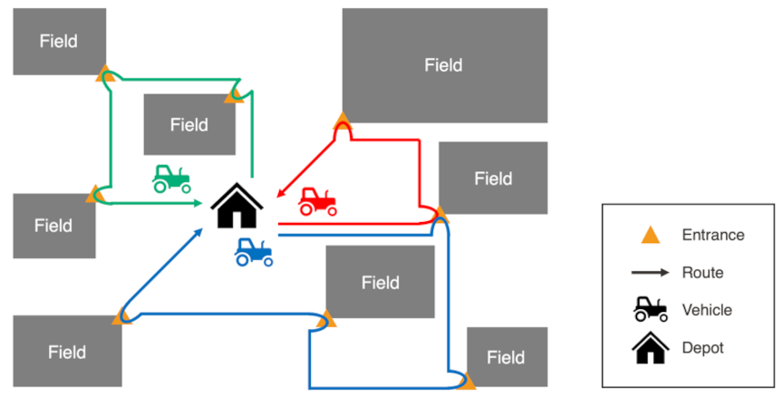
Fig. 1. Overview of the target problem in field-based mobile machines.
2. Problem Settings
2.1. Target Problem
First, we use the term task allocation in a broad sense to refer to the combined process of assigning agricultural fields to machines and determining the sequence in which each machine visits these fields. Although this process is commonly framed as a VRP, especially in the form of an SDVRP, we interpret such routing-based formulations as a means of realizing practical field-level task allocation. Therefore, unless otherwise specified, we treat the outcome of route planning as a form of task allocation tailored to multi-machine agricultural operations.
This study focuses on the fundamental agricultural task of tillage, specifically exploring the process of task assignments to multiple agricultural machines and the generation of travel routes between fields. Although extensive research has addressed intra-field route planning (e.g., 21,16), our study focuses on inter-field task assignment and routing. Instead, the costs associated with field operations are incorporated as given parameters; these have been derived from previous studies, effectively treating intra-field route generation as outside the scope of this research. The farmland in question is structured with a depot, multiple fields, and roads; like a real farmland, each field has a single designated entrance. Machines are required to travel only on roads during inter-field movements and cannot traverse through fields to access other fields. Each machine starts its day from the depot, begins working upon reaching a field, and returns to the depot after completing all the assigned tasks. The farmland environment is considered sufficiently sparse, eliminating the need to factor in the costs associated with mutual avoidance when machines operate in close proximity. Fig. 1 provides a visual overview of the target problem, illustrating the layout of the depot, fields, roads, and typical paths that machines use between these components.
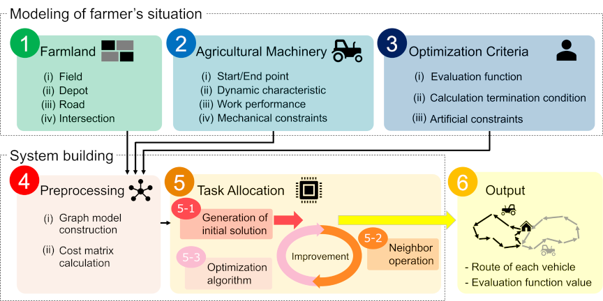
Fig. 2. Proposed versatile task allocation framework.
2.2. Formulation
The objective is to assign and route multiple agricultural machines to cover all the designated fields while minimizing the total travel distance and satisfying the operational constraints. The problem is formulated as follows.
Objective function: Minimize total travel distance
Subject to
departure and return to depot:
field assignment:
demand satisfaction:
flow continuity (arrival):
flow continuity (departure):
subtour elimination:
binary constraints for field assignment:
binary constraints for routing:
Decision Variables and Parameters
-
\(x_{ijk}\):
1 if machine \(k\) travels directly from node \(i\) to node \(j\); 0 otherwise.
-
\(y_{ik}\):
1 if machine \(k\) is assigned to field \(i\); 0 otherwise.
-
\(z_{ik}\):
Amount of work done by machine \(k\) in field \(i\).
-
\(m\):
Total number of machines.
-
\(n\):
Total number of fields.
-
\(d_i\):
Demand for tasks in the field \(i\).
-
\(c_{ij}\):
Travel cost from node \(i\) to node \(j\), where node \(0\) represents the depot and nodes \(1\) through \(n\) represent the fields.
Constraint Explanations
Equation (1) minimizes the total travel cost.
Equation (2) ensures that each machine starts and ends at the depot.
Equation (3) assigns each field to at least one machine.
Equation (4) ensures that the total work done satisfies the demands of each field.
Equations (3) and (4) together enable split delivery.
Equation (5) ensures that if a machine visits a field, it has arrived from another node.
Equation (6) ensures that it must also leave.
Equation (7) eliminates subtours.
Equations (8) and (9) define binary decision variables.
3. Proposed Versatile Task Allocation Framework
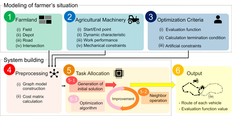
We developed a system that systematically incorporates the critical elements for effective task allocation in agricultural settings. To this end, we first organized the critical elements required for practical applications. The proposed framework, depicted in Fig. 2, comprises the following six steps: Steps 1–3 involve the conditioning process for problem setting based on interviews with farmers and the related documents 11. Steps 4 and 5 focus on building a task allocation system structured through a comprehensive survey of the existing research in the field.
-
Step 1.
Modeling the Farmland Input the information pertaining to (i) fields, (ii) depots, (iii) roads, and (iv) intersections to model the farmland.
-
Step 2.
Modeling the Agricultural Machinery The movement of machinery in agricultural work can be categorized into four stages: departure, travel, fieldwork, and arrival. To model the machinery, we defined (i) the start/end points for departure/arrival, (ii) dynamic characteristics for travel, (iii) work performance for fieldwork, and (iv) mechanical constraints. The dynamic characteristics (ii) encompass elements such as speed and acceleration/deceleration of the machinery. Mechanical constraints (iv) cover aspects such as road accessibility, capacity constraints, and coordination with other machinery.
-
Step 3.
Modeling the Optimization Criteria Appropriate modeling of the optimization criteria for task allocation is crucial. For instance, the emphasis on elements in route planning and the required accuracy of output routes may differ among farmers. Therefore, we established the following: (i) evaluation functions that consider the optimization criteria, (ii) conditions for terminating the calculations, and (iii) artificial constraint conditions. Artificial constraint conditions incorporate constraints such as maximum working hours and load distribution among the machinery.
-
Step 4.
Preprocessing Based on the information provided in Steps 1–3, we (i) constructed a graph model of the farmland and (ii) calculated the cost matrix essential for task allocation and improvement. Split delivery is enabled by representing each field as multiple subnodes (Section 4.1.1), allowing a partial assignment to the machines. The optimization algorithms operate on this graph and support multiple visits per field.
-
Step 5.
Task Allocation Task allocation can be subdivided into three sub-steps:
(1) Initial Solution Generation Construct an initial solution that satisfies the constraints.
(2) Neighbor Operation Perform certain operations on the input solution to generate neighbor solutions.
(3) Optimization Algorithm Improve the solution through optimization algorithms. Metaheuristics are applied in this part.
-
Step 6.
Output Output the best solution derived in Step 5. Depending on the situation, appropriate information is provided in an appropriate format.
By consolidating common structural elements, such as inputs, outputs, and algorithms, across diverse methods, the proposed framework not only clarifies the positions of both past and future research in this domain but also establishes a foundational basis for unified discourse. Previous studies have often focused on partial sub-problems, making it difficult to compare and discuss different approaches. By contrast, this framework provides a means for organizing the existing knowledge and anticipating future developments, thereby functioning as a guideline that highlights the essential considerations for system development, particularly for those aiming to implement future routing systems. Notably, modeling farmland and constructing a system in alignment with this framework facilitates the creation of an optimization system for task allocation. Among the key contributions is “Step 3: Modeling the Optimization Criteria,” an element which was previously overlooked or only superficially addressed without meaningful comparative analysis. In addition, by examining various scenarios and algorithms, the framework clarifies the components that require adaptation, simplified modifications, and customization. Consequently, adopting this framework ensures a comprehensive consideration of all the critical elements for practical applications, ultimately promoting a more effective system development.
This modular framework is designed to be universal and scalable. Each step, ranging from farmland modeling to task assignment, is independent and loosely coupled, allowing adaptation to various agricultural contexts. For example, Step 1 can incorporate GIS-based farmland data from different countries, Step 2 can be adjusted to different machine types or implements, and Step 3 accommodates diverse farmer preferences and constraints. The algorithmic modules in Steps 5 and 6 can be easily extended to include new heuristics or real-time optimization schemes as the technology evolves. This flexibility ensures the applicability of the framework not only to tillage but also to tasks, such as spraying, harvesting, and weeding. Consequently, the framework serves as a reusable platform for a wide range of task allocation problems in agriculture.
4. System Development and Computer Simulation
4.1. Simulation Overview
In this study, farmland conditions are classified based on the two primary factors that influence algorithm selection: the number of nodes, which reflects the scale of the farmland, and the maximum calculation time. As previously discussed, the scale of farmland can range from small to large, whereas calculation times may vary significantly depending on whether the solution quality is prioritized for preplanning or near-real-time planning is required to adjust for errors and other factors. To determine the optimal algorithms and associated hyperparameters for each condition, we modeled the farmland and constructed a system according to the proposed framework, followed by computer simulations. The best hyperparameters for each scenario are identified using a grid search 22. This approach establishes that the algorithms and hyperparameters vary across different farmland conditions, and it identifies the most effective optimization methods for each scenario. The system is implemented in Python, and the simulations are run on a computer with the following specifications: AMD EPYC 7513 32-Core Processor @2.6 GHz and 32 GB of RAM.
The remainder of Section 4 is organized as follows: Sections 4.1.1, 4.1.2, and 4.1.3 discuss the key considerations in executing the simulations. Section 4.2 details the modeling of the farmland and the system construction according to the framework, and Section 4.3 presents the simulation results.
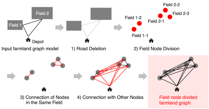
Fig. 3. Field node-divided farmland graph construction process.
4.1.1. Field Node-Divided Farmland Graph
To optimize task allocation, scenarios where tasks within a single field are shared among multiple machines must be accounted for. In practical agricultural operations, the number of machines working in a single field is limited. Therefore, when treating fields as nodes, segmenting the nodes based on the maximum number of machines that can operate in each field is sufficient. We propose a method to model farmland by reconstructing a graph; this graph is henceforth referred to as a field-node-divided farmland graph. This approach facilitates the derivation of routes that accommodate multiple agricultural machines operating in a single field, thus treating the problem as an SDVRP. The transformation of a simply modeled farmland graph into a field-node-divided farmland graph involves the following four steps:
-
Road deletion: The edges corresponding to roads connecting fields and the depot are deleted. The information on the deleted edges is recorded for later reference.
-
Field node division: The nodes corresponding to the fields are divided amongst the maximum number of machines that can operate in these fields, generating multiple nodes for a given field.
-
Connection of nodes in the same field: Connect the nodes corresponding to the same field with edges of zero distance.
-
Connection with other nodes: Connect the nodes corresponding to fields with nodes corresponding to other fields and the depot using edges representing roads. The connections are established by referring to the road information recorded in Step 1 and assigning appropriate attributes to the edges. This operation ensures that each node is connected to all other nodes.
Figure 3 illustrates the process of constructing the field-node-divided farmland graph.
4.1.2. Algorithm Selection
To develop a versatile task allocation system, it is important to comprehensively extract the possible SDVRP solution algorithms, implement each method, and establish a framework for selecting an appropriate algorithm based on a specific problem. Considering the various metaheuristics and prior studies related to VRP, such as 23,24, metaheuristics can be categorized into evolutionary computations and other methods. Further subdivisions of evolutionary computations include swarm intelligence and evolutionary algorithms. A classification diagram of these algorithms is shown in Fig. 4.
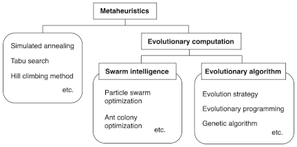
Fig. 4. Classification of metaheuristics.
In this study, we selected representative algorithms from each domain and comprehensively implemented metaheuristics to compare the simulation results and determine the most appropriate solution algorithms and their hyperparameters based on the conditions in the farmland. Specifically, we implemented four metaheuristic algorithms: local search, SA 25, genetic algorithm (GA) 26, ant colony optimization (ACO) 27 in standard forms. For the local search and SA, we adopted the insertion neighbor approach 28, and for GA, we utilized the order crossover method 29. The parameters are tuned using a grid search.
Table 1. Characteristics of each farmland.

4.1.3. Settings of Agricultural Field
To reflect realistic field conditions, five types of virtual farmlands were created based on the agricultural statistics for Japan and prior studies 30,15. These farmlands, ranging in scale from extra-small to extra-large, vary in number of individual fields, total areas, and layouts. Each field has a fixed area (30 a) and one entrance. A maximum of two machines can be operated in the field.
All the farmlands follow a grid-based road structure with a centrally located depot. The distances between the fields and the depot are represented by a matrix, allowing the internal network structure to be abstracted during optimization.
Table 1 summarizes the characteristics of the farmlands. “Model” indicates farmer types, which affect field size and number. These differences influence the routing complexity and algorithm behavior.
Figure 5 shows the schematic of a small farmland area. For clarity, a simplified schematic with grid-like fields and a central depot is shown. While this idealized layout is useful for verifying the algorithm performance, the proposed framework is designed to accommodate irregular field shapes and varied topologies based on real-world geographical data.
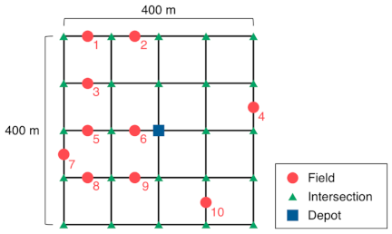
Fig. 5. Schematic of small farmland (red subscripts represent the number assigned to each field).
Although the five virtual farmland types used in this study are based on Japanese agricultural statistics and representative farming models, the proposed modeling method is not limited to the Japanese setting. The structure of Step 1 in the framework allows farmland input to be constructed using available geographic or cadastral information. For example, GIS data from European or North American farms with irregularly shaped fields and decentralized depots can be directly incorporated. In addition, the distance matrix abstraction enables the internal network structure to be replaced by any road topology or field connectivity, making the system adaptable to different regional characteristics.
4.2. Development of Systems According to the Proposed Framework
This section details the modeling of the farmland and the construction of the system according to the proposed framework.
-
Step 1.
Modeling the Farmland The simulation targets five types of farmland: extra small, small, medium, large, and extra-large, as described in Section 4.1.3. The attributes of the fields, depots, roads, and intersections for each farmland type are summarized in Table 2.
Table 2. Attributes of farmland components.

-
Step 2.
Modeling the Agricultural Machinery Assuming the use of three machines for all the farmlands, the parameters for the machinery are set as follows. All machines start from and return to the depot. The working speed within the field is set to 0.5 a/min. The travel speeds are differentiated, with two machines traveling at 250 m/min and one at 125 m/min. All machines could travel in both directions on all roads. The simulation settings emulate manual and autonomous operations. In practice, the in-field working speeds of these modes are often comparable, whereas autonomous travel speeds tend to be configured more conservatively for safety outside the field. Our parameters reflected these general trends.
-
Step 3.
Modeling the Optimization Criteria Previous studies on task allocation systems predominantly focused on minimizing the total travel distance when evaluating routing decisions, for instance, 21,3,20,6, and considered only this metric. However, while distance reduction is undoubtedly important, farmers often prioritize minimizing the time required to complete all tasks, as highlighted by 16. Therefore, striking a balance between efficiency in terms of distance and practicality in terms of completion time is essential. In this simulation, mechanical and human costs are considered. The evaluation function \(f\) is set as follows:
\begin{align} f &= w_d \frac{D}{v} + w_t T, \\ \end{align}\begin{align} w_d &= w_t = 1, \end{align}where

Eq. (10) defines the evaluation function, and Eq. (11) specifies that the weights are set to be equal. The variable \(D\) measures the mechanical cost, accounting for machine wear and tear and fuel consumption, while \(T\) represents the human cost, reflecting the actual working time. The variable \(v\) is introduced to standardize the units of the evaluation function over time. This function facilitates the derivation of routes that balance the total travel distance of the agricultural machinery with the working time of the farmer. The computation times for the simulation were considered for five variations: 0.1, 1, 10, 100, and 1,000 s.
-
Step 4.
Preprocessing First, a cost matrix was calculated. The shortest path between each depot and the field is calculated using the Floyd–Warshall algorithm 31, resulting in the distance matrix \(D\):
\begin{equation} D = \begin{bmatrix} d_{11} & \cdots & d_{1n}\\ \vdots & \ddots & \vdots\\ d_{n1} & \cdots & d_{nn} \end{bmatrix}, \end{equation}where \(d_{ij}\) represents the distance from point \(i\) to point \(j\). \(n\) is the total number of fields and depots.
Next, for a machine \(\alpha\), derive the time matrix \(T_\alpha\) from the distance matrix \(D\) based on the travel speed \(v_\alpha\):
\begin{equation} T_\alpha = \frac{D}{v_\alpha}. \end{equation}Subsequently, the work-time information in each field is stored in the work-time matrix \(W_\alpha\):
\begin{equation} W_\alpha = \left[ w_1\ w_2\ \cdots\ w_n \right], \end{equation}where \(w_i\) represents the work time at point \(i\).
Additionally, the passability matrix \(P_\alpha\) is created to indicate whether machine \(\alpha\) can travel on a certain road:
\begin{equation} P_\alpha = \begin{bmatrix} p_{11} & \cdots & p_{1n}\\ \vdots & \ddots & \vdots\\ p_{n1} & \cdots & p_{nn} \end{bmatrix}, \end{equation}where \(p_{ij}\) represents the passability from point \(i\) to point \(j\), with \(0\) indicating passable and \(\infty\) indicating impassable.
Finally, the above matrices are combined to construct the cost matrix \(C_\alpha\) for machine \(\alpha\) when moving from point \(i\) to point \(j\):
\begin{align} C_{\alpha k} &= T_{\alpha k} + W_\alpha + P_{\alpha k}, \\ \end{align}\begin{align} C_\alpha &= \begin{bmatrix} c_{11} & \cdots & c_{1n} \\ \vdots & \ddots & \vdots \\ c_{n1} & \cdots & c_{nn} \end{bmatrix}, \end{align}where \(C_{\alpha k}\), \(T_{\alpha k}\), and \(P_{\alpha k}\) represent the \(k\)-th row of \(C_{\alpha}\), \(T_{\alpha}\), and \(P_{\alpha}\), respectively. The \(ij\)-th component of \(C_{\alpha}\) contains the cost information for moving from point \(i\) to \(j\). If \(c_{ij}\) is infinite, movement from point \(i\) to \(j\) is impossible. To evaluate the function, distance matrix \(D\) is used to calculate the total travel distance, whereas cost matrix \(C\) is utilized to calculate the makespan.
As outlined in Section 4.1.1, a field node-divided farmland graph is constructed by converting a simple farmland model graph. Given that the maximum number of machines working in a single field is two, each field is divided into two nodes.
-
Step 5.
Task Allocation
-
Step 5-1.
Initial Solution Generation A randomly generated initial solution is used for the simulations. For local search, SA, and ACO, the same initial solutions are utilized. For GA, we generate as many initial solutions as the population size, which is set as a hyperparameter. Three initial solutions are generated, meaning three simulations are run for each algorithm and for each set of hyperparameters.
-
Step 5-2.
Neighbor Operations As detailed in Section 4.1.2, insertion neighbors are generated for the local search and SA. For the GA, neighbor solutions are generated using three specific methods: selection by the roulette wheel method, crossover through Order Crossover, and mutation by the swap neighbor method. In ACO, neighbor solutions are probabilistically generated based on the pheromone trails left by virtual ants.
-
Step 5-3.
Optimization Algorithm The four types of optimization algorithms mentioned in Section 4.1.2: local search, SA, GA, and ACO, are utilized. The hyperparameters for each algorithm are set as outlined in Table 3. A grid search was conducted across 129 configurations, which were distributed as follows: one configuration for the local search, 35 for SA, 45 for GA, and 48 for ACO. These hyperparameters are dimensionless quantities because they represent the virtual parameters within the algorithm.
-
Step 5-1.
-
Step 6.
Output The best solution is the output at the point at which the predefined maximum computation time has elapsed.
Table 3. Hyperparameters of each algorithm.

4.3. Simulation Results
The system was successfully implemented and the simulation was executed, resulting in effective task allocation. The farm size and layout vary by type, affecting the route length and suitable algorithms. As an illustration of the simulation results, Fig. 6 displays the output of the best solution from SA with an initial temperature of 20 and a cooling rate of 0.9999999, tailored for a small farmland under a maximum computation time of 1,000 s. The tasks assigned to each machine are listed in Table 4. This demonstrates that the system, constructed in accordance with the proposed framework, effectively derived routes that enabled sharing of certain field tasks among multiple machines, thereby achieving efficient task allocation and route optimization.
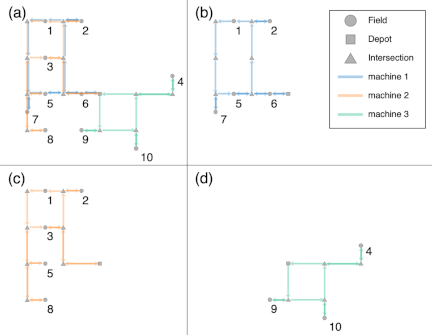
Fig. 6. Example of a generated route (farmland: small, algorithm: SA (initial temperature \(= 20\), cooling rate \(= 0.9999999\))): (a) overview of the route, (b) route of the first machine (speed \(= 250\) m/min), (c) route of the second machine (speed \(= 250\) m/min), and (d) route of the third machine (speed \(= 125\) m/min).
Table 4. Task assignment results (farmland: small, algorithm: SA (initial temperature \(=20\), cooling rate \(= 0.9999999\))).

Next, the average evaluation function values were calculated from the three initial solutions for each combination of the optimization method and hyperparameters. These values were used to identify the best optimization method and hyperparameter combination for different farmland sizes and maximum computation times, as shown in Fig. 7. In this figure, “–” indicates that no algorithm could generate a route within the computation time or that fewer than 10 iterations occurred, which resulted in insufficient solution improvement cycles. The hyperparameters for each optimization method are specified in parentheses below the name of each method in the corresponding row. For SA, the hyperparameters included the initial temperature (first component) and cooling rate (second component). For GA, the hyperparameters are the population size (first component), selection rate (second component), and crossover rate (third component). For ACO, the hyperparameters are the evaporation rate (first component), initial pheromone amount (second component), and deposited pheromone amount (third component). If multiple algorithms are noted in a single cell, it indicates that they produce the best routes with equivalent evaluation function values. When different settings of hyperparameters yielded the same evaluation function value for an optimization method, the representative set was chosen based on the smallest value of the first component. If these were equal, then the second component was considered, and so forth.
Across different farmland sizes, SA and GA were more effective in smaller scenarios, whereas local search dominated the performance in larger-scale tasks.
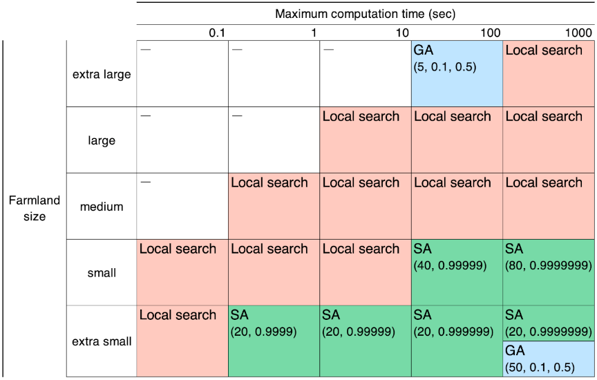
Fig. 7. Best optimization method and hyperparameter combination according to farmland size and maximum computation time.
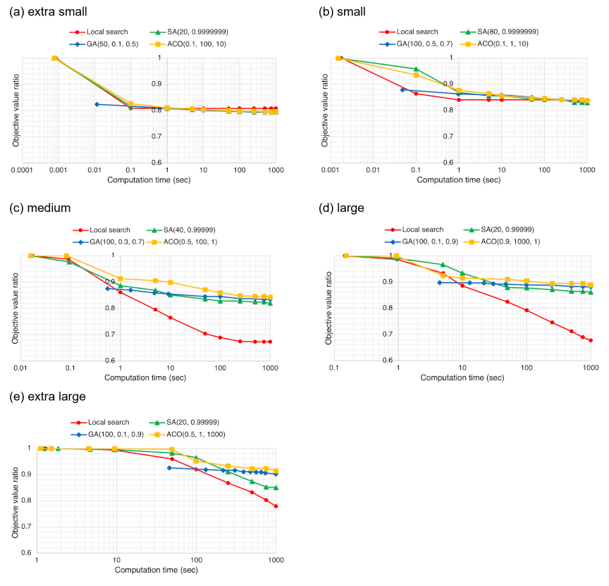
Fig. 8. Comparison of evaluation function value transitions for each farmland under the hyperparameter conditions producing the best solutions at 1,000 s: (a) extra-small farmland, (b) small farmland, (c) medium farmland, (d) large farmland, and (e) extra-large farmland.
Figure 8 illustrates performance transitions across farmland sizes. Overall, SA and GA performed well for smaller farms, whereas local search was the most effective in larger-scale or time-constrained scenarios.
To assess the sensitivity of the performance to hyperparameter settings, we analyzed how changes in key parameters influenced the evaluation function values under different farmland and time conditions. For SA, the performance was particularly sensitive to the cooling rate, where values closer to 1.0 generally improved the solution quality given sufficient computation time. For the GA, the population size significantly affected performance, especially in small-scale farmlands. In contrast, ACO exhibited high variability with no consistent trend across the parameter changes. These observations underscore the importance of tuning, particularly for the SA and GA, and highlight the need to select algorithms whose key parameters can be reliably optimized.
5. Discussion
In this section, we assess the proposed framework by examining the tradeoffs in the simulation results, focusing on the balance between operational efficiency and cost. As a starting point, it is essential to consider how the application of the proposed framework in a simulation setting has opened avenues for broader exploration. While the current simulation employs only basic algorithms, the framework structure readily accommodates the integration of various existing and future algorithms. This flexibility allows for systematic comparison and in-depth discussion, paving the way for a more informed selection and combination of methods in subsequent implementations. Notably, “Step 3: Modeling the Optimization Criteria” brings a dimension that has been minimally addressed in previous work, thereby enhancing the representation of real-world decision-making processes. Moreover, the capability to examine different scenarios or algorithms clarifies the points of adaptation and simplifies the modification and customization processes. This flexibility not only supports tillage, but also has potential applications in a variety of agricultural tasks, such as pesticide application and seeding. The framework fosters the evolution of more versatile, context-sensitive, and effective task allocation systems by creating an environment in which multiple approaches can be tested, critiqued, and refined.
Next, the computer simulation results are reviewed. The simulations indicated that both SA and local search are effective across various farmland scenarios. Specifically, SA performs effectively in small farmlands given the ample computation time, whereas local search excels in larger farmlands or under restricted computation times. This efficacy stems from their simplicity, which allows for more frequent solution enhancements per unit time compared to the GA and ACO. Furthermore, while SA aims for the global optimum by permitting solution deterioration, the local search tends to become trapped in the local optima. For large farmlands, the evaluation function values of the local search do not converge, suggesting that the search range is too broad to achieve a local optimum; hence, it is superior to SA in these instances. In contrast, the GA shows potential under specific conditions, although ACO is less effective than the other algorithms.
In terms of SA, setting the initial temperature between 20 and 40 and the cooling rate at approximately 0.9999–0.9999999 was found optimal, providing a guideline for realistic settings. For GA, larger population sizes have proven advantageous, which aligns with past findings emphasizing solution diversity. However, trends in the selection and crossover rates were indeterminate, highlighting the need for meticulous hyperparameter tuning according to specific farmland scenarios. Overall, these results clearly demonstrate that the optimal optimization method varies depending on the circumstances of the farm. Furthermore, the simulations successfully identified the most effective optimization approach for each scenario, providing practical insights into selecting an appropriate method tailored to specific farming conditions.
Finally, we discuss the limitations of this study. The proposed framework addressed only static task allocation and did not accommodate dynamic situations that may necessitate different components. Although a comprehensive selection of computer simulation algorithms has been tested, several variants remain unexamined. In Step 5 of the framework, the initial solution generation (Step 5-1) was random and limited to three, with simple neighbor operations (Step 5-2) employed. Expanding the number of initial solutions and conducting more thorough analyses of the average results could bolster reliability. Furthermore, although more sophisticated solution construction methods and metaheuristics could potentially yield better outcomes, this study’s primary contribution lies in defining a framework that enables a more comprehensive discourse. By leveraging this framework, it is possible to develop systems that more holistically account for the conditions faced by individual farmers, as illustrated by the simulations in this study.
Additionally, the hyperparameter tuning approach utilized a grid search, which, while comprehensive, does not necessarily pinpoint the optimal set and becomes labor-intensive during fine-tuning. Integrating advanced tuning methods such as Bayesian optimization 32, can significantly enhance the simulation efficiency. Looking ahead, the goal should be to move beyond virtual farmland simulations and conduct empirical tests in real-world agricultural settings, further validating and refining both the framework and resulting systems.
This study is limited to virtual farmland simulations. Although the framework can incorporate real-world data such as GIS maps and speed records, field validation remains a topic for future research. To enhance its practical relevance, we plan to apply the system to actual farmlands and conduct small-scale trials.
6. Conclusions
In this study, we developed a framework for a versatile task allocation system tailored to agricultural requirements. Using this framework, we constructed a task allocation system and identified optimal optimization methods and hyperparameters for various farming conditions through computer simulations. These simulations categorized farming conditions by farmland scale and maximum computation time, and determined the most suitable hyperparameters using a grid search. The results revealed that SA is the most effective for small farmlands with extended computation times, whereas local search excels for large farmlands and constrained computation times.
In future, we aim to explore a broader spectrum of farming conditions and incorporate a more diverse array of algorithms into our simulations. Future work will focus on identifying specific feature variables, such as field geometry and fleet size, to establish the criteria for optimal algorithm selection under diverse farming conditions. We also intend to advance the task allocation system through field trials on farmland. In addition, for practical deployment in real-world agricultural settings, future research should extend the proposed framework to incorporate heterogeneity in machine-implement combinations. In such scenarios, variations in the working speed, maneuverability, and soil compaction 5, stemming from differences in machine scale, must be explicitly modeled to ensure a more realistic task allocation for mixed fleets of agricultural machinery.
- [1] C. Ju, J. Kim, J. Seol, and H. I. Son, “A review on multirobot systems in agriculture,” Computers and Electronics in Agriculture, Vol.202, Article No.107336, 2022. https://doi.org/10.1016/j.compag.2022.107336
- [2] A. Utamima and A. Djunaidy, “Agricultural routing planning: A narrative review of literature,” Procedia Computer Science, Vol.197, pp. 693-700, 2022. https://doi.org/10.1016/j.procs.2021.12.190
- [3] R. Cao, S. Li, Y. Ji, Z. Zhang, H. Xu, M. Zhang, M. Li, and H. Li, “Task assignment of multiple agricultural machinery cooperation based on improved ant colony algorithm,” Computers and Electronics in Agriculture, Vol.182, Article No.105993, 2021. https://doi.org/10.1016/j.compag.2021.105993
- [4] S. Fountas, C. G. Sørensen, Z. Tsiropoulos, C. Cavalaris, V. Liakos, and T. Gemtos, “Farm machinery management information system,” Computers and Electronics in Agriculture, Vol.110, pp. 131-138, 2015. https://doi.org/10.1016/j.compag.2014.11.011
- [5] W. C. T. Chamen, A. P. Moxey, W. Towers, B. Balana, and P. D. Hallett, “Mitigating arable soil compaction: A review and analysis of available cost and benefit data,” Soil and Tillage Research, Vol.146, Part A, pp. 10-25, 2015. https://doi.org/10.1016/j.still.2014.09.011
- [6] A. Utamima and T. Reiners, “Navigating route planning for multiple vehicles in multifield agriculture with a fast hybrid algorithm,” Computers and Electronics in Agriculture, Vol.212, Article No.108021, 2023. https://doi.org/10.1016/j.compag.2023.108021
- [7] M. Umemoto, “Actual conditions of interdistrict and inter-field movements associated with field dispersion: A case study of large-scale rice farming management in western Ibaraki prefecture,” Kanto Tokai J. of Farm Management, Vol.100, pp. 55-58, 2010 (in Japanese).
- [8] M. Dror and P. Trudeau, “Split delivery routing,” Naval Research Logistics, Vol.37, Issue 3, pp. 383-402, 1990. https://doi.org/10.1002/nav.3800370304
- [9] M. Dror, G. Laporte, and P. Trudeau, “Vehicle routing with split deliveries,” Discrete Applied Mathematics, Vol.50, Issue 3, pp. 239-254, 1994. https://doi.org/10.1016/0166-218X(92)00172-I
- [10] D. D. Bochtis and C. G. Sørensen, “The vehicle routing problem in field logistics part I,” Biosystems Engineering, Vol.104, Issue 4, pp. 447-457, 2009. https://doi.org/10.1016/j.biosystemseng.2009.09.003
- [11] J. Conesa-Muñoz, J. M. Bengochea-Guevara, D. Andujar, and A. Ribeiro, “Route planning for agricultural tasks: A general approach for fleets of autonomous vehicles in site-specific herbicide applications,” Computers and Electronics in Agriculture, Vol.127, pp. 204-220, 2016. https://doi.org/10.1016/j.compag.2016.06.012
- [12] H. Seyyedhasani and J. S. Dvorak, “Using the vehicle routing problem to reduce field completion times with multiple machines,” Computers and Electronics in Agriculture, Vol.134, pp. 142-150, 2017. https://doi.org/10.1016/j.compag.2016.11.010
- [13] J. Thomas, “Property rights, land fragmentation and the emerging structure of agriculture in central and eastern European countries,” eJADE Electronic J. of Agricultural and Development Economics, Vol.3, No.2, pp. 225-275, 2006.
- [14] C. Amiama, N. Cascudo, L. Carpente, and A. Cerdeira-Pena, “A decision tool for maize silage harvest operations,” Biosystems Engineering, Vol.134, pp. 94-104, 2015. https://doi.org/10.1016/j.biosystemseng.2015.04.004
- [15] Mitsubishi Research Institute, “Are All Rice Farmers in the Red?,” Food Security and Agriculture, Vol.3, 2023 (in Japanese).
- [16] H. Seyyedhasani and J. S. Dvorak, “Dynamic rerouting of a fleet of vehicles in agricultural operations through a dynamic multiple depot vehicle routing problem representation,” Biosystems Engineering, Vol.171, pp. 63-77, 2018. https://doi.org/10.1016/j.biosystemseng.2018.04.003
- [17] T. Oksanen and A. Visala, “Coverage path planning algorithms for agricultural field machines,” J. of Field Robotics, Vol.26, Issue 8, pp. 651-668, 2009. https://doi.org/10.1002/rob.20300
- [18] I. A. Hameed, D. D. Bochtis, and C. G. Sorensen, “Driving Angle and Track Sequence Optimization for Operational Path Planning Using Genetic Algorithms,” Applied Engineering in Agriculture, Vol.27, No.6, pp. 1077-1086, 2011. https://doi.org/10.13031/2013.40615
- [19] M. Graf Plessen, “Optimal in-field routing for full and partial field coverage with arbitrary non-convex fields and multiple obstacle areas,” Biosystems Engineering, Vol.186, pp. 234-245, 2019. https://doi.org/10.1016/j.biosystemseng.2019.08.001
- [20] C. Gracia, B. Velázquez-Martí, and J. Estornell, “An application of the vehicle routing problem to biomass transportation,” Biosystems Engineering, Vol.124, pp. 40-52, 2014. https://doi.org/10.1016/j.biosystemseng.2014.06.009
- [21] M. Vahdanjoo, K. Zhou, and C. A. G. Sørensen, “Route Planning for Agricultural Machines with Multiple Depots: Manure Application Case Study,” Agronomy, Vol.10, Issue 10, Article No.1608, 2020. https://doi.org/10.3390/agronomy10101608
- [22] T. Yu and H. Zhu, “Hyper-parameter optimization: A review of algorithms and applications,” arXiv preprint, arXiv:2003.05689, 2020. https://doi.org/10.48550/arXiv.2003.05689
- [23] A. E. Ezugwu, A. K. Shukla, R. Nath, A. A. Akinyelu, J. O. Agushaka, H. Chiroma, and P. K. Muhuri, “Metaheuristics: A comprehensive overview and classification along with bibliometric analysis,” Artificial Intelligence Review, Vol.54, pp. 4237-4316, 2021. https://doi.org/10.1007/s10462-020-09952-0
- [24] G. D. Konstantakopoulos, S. P. Gayialis, and E. P. Kechagias, “Vehicle routing problem and related algorithms for logistics distribution: A literature review and classification,” Operational Research, Vol.22, pp. 2033-2062, 2022. https://doi.org/10.1007/s12351-020-00600-7
- [25] S. Kirkpatrick, C. D. Gelatt, Jr., and M. P. Vecchi, “Optimization by Simulated Annealing,” Science, Vol.220, Issue 4598, pp. 671-680, 1983. https://doi.org/10.1126/science.220.4598.671
- [26] J. H. Holland, “Adaptation in Natural and Artificial Systems: An Introductory Analysis with Applications to Biology, Control, and Artificial Intelligence,” MIT Press, 1992. https://doi.org/10.7551/mitpress/1090.001.0001
- [27] M. Dorigo, V. Maniezzo, and A. Colorni, “Ant system: optimization by a colony of cooperating agents,” IEEE Trans. on Systems, Man, and Cybernetics, Part B (Cybernetics), Vol.26, Issue 1, pp. 29-41, 1996. https://doi.org/10.1109/3477.484436
- [28] N. M. E. Normasari, V. F. Yu, C. Bachtiyar, and Sukoyo, “A Simulated Annealing Heuristic for the Capacitated Green Vehicle Routing Problem,” Math. Probl. Eng., pp. 1-18, 2019. https://doi.org/10.1155/2019/2358258
- [29] J. Ochelska-Mierzejewska, A. Poniszewska-Marańda, and W. Marańda, “Selected Genetic Algorithms for Vehicle Routing Problem Solving,” Electronics, Vol.10, Issue 24, Article No.3147, 2021. https://doi.org/10.3390/electronics10243147
- [30] Ministry of Agriculture, Forestry and Fisheries, “2020 Census of Agriculture and Forestry in Japan Census Results Report,” 2020.
- [31] R. W. Floyd, “Algorithm 97: Shortest path,” Communications of the ACM, Vol.5, Issue 6, p. 345, 1962. https://doi.org/10.1145/367766.368168
- [32] H. Alibrahim and S. A. Ludwig, “Hyperparameter Optimization: Comparing Genetic Algorithm against Grid Search and Bayesian Optimization,” 2021 IEEE Congress on Evolutionary Computation (CEC), pp. 1551-1559, 2021. https://doi.org/10.1109/CEC45853.2021.9504761
This article is published under a Creative Commons Attribution-NoDerivatives 4.0 Internationa License.