Paper:
Design of Impedance Control and Position Tracking Control for Nonlinear Hydraulic Arms
Kota Kumabe*, Satoru Sakai*
 , Yushiro Hayakawa*, Yanbin Zhang*, and Yoshiyuki Uchikawa**
*Department of Mechanical Engineering, Shinshu University
4-17-1 Wakasato, Nagano, Nagano 380-8553, Japan
**Department of Agricultural and Life Sciences, Shinshu University
8304 Minamiminowa, Kamiina, Nagano 399-4598, Japan

This paper discusses desired disturbance response model + desired reference response model for simultaneously satisfying an impedance control and a position orientation tracking control for nonlinear hydraulic arms. First, we review hydraulic cylinder dynamics with nonlinear pressure dynamics. Second, through the reviewed hydraulic cylinder dynamics and an existing controller design procedure, we discuss two desired models for achieving an impedance control and a position orientation tracking control simultaneously. Finally, the effectiveness of the proposed desired models is confirmed by a preliminary indoor experiment including a simulated open channel.
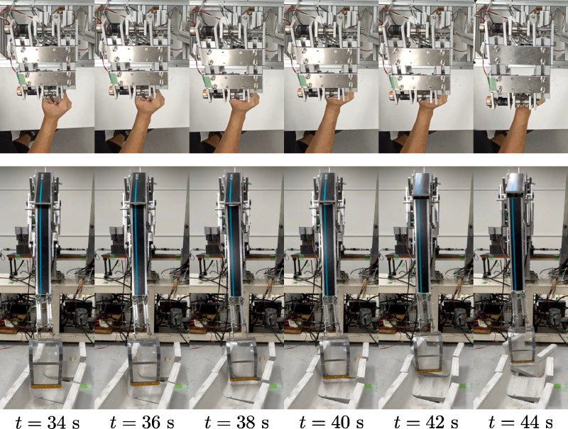
Experiments using a master-follower system (conventional curved section)
1. Introduction
Hydraulic arms have been used in the extreme environments such as construction, agriculture, and demining, among others due to their higher robustness and significantly larger power to weight ratio compared with electric arms. In mountainous agricultural works, reliable water conveyance requires periodic canal cleaning; neglected canals often become silted by wildlife digging and by inflows of sediment and dead bamboo, frequently necessitating manual labor. Although mechanization with hydraulic excavators is advancing, bucket contact with channel walls or the bed is likely in curved reaches or on uneven terrain, creating a risk of structural damage. The position and attitude control of hydraulic excavators commonly employs position error-based PID (e.g., 1) tracking loops due to their implementation simplicity and established practice. Such position control prioritizes desired tracking and typically does not treat interaction properties such as apparent stiffness and apparent damping as explicit design objectives. Consequently, when contact forces predominate, it becomes challenging to manipulate the interaction to manifest the desired bandwidth characteristics. The capacity of disturbance observers (e.g., 2) to enhance tracking is predicated on their ability to estimate and compensate for friction and external load forces. However, their primary function is disturbance rejection, and they do not, in and of themselves, provide a framework for specifying the interaction band shaping required during contact. In contrast, impedance control is well suited to contact tasks; by shaping the bandwidth of apparent stiffness and damping, it may suppress contact forces while maintaining tracking performance. However, in harsh environments the environmental durability and overload tolerance of high-sensitivity force sensors are problematic, motivating force sensorless implementations. In pneumatic systems, force sensorless impedance control has been demonstrated (e.g., 3,4). While pneumatic and hydraulic systems share closely related governing dynamics and are therefore conceptually analogous, representative hydraulic implementations of impedance control (e.g., 5) typically assume force sensing. Consequently, sensorless implementations for hydraulics especially under high-rigidity contact remain insufficiently studied. This work addresses that gap by proposing a controller that simultaneously achieves force sensorless impedance control and position tracking using a hydraulic arm consisting of ready-made components. We evaluate performance with respect to a desired model and a disturbance response model under unknown external forces. In addition, we conduct preliminary indoor experiments emulating waterway cleaning and assess effectiveness on non-contact and side-wall-contact trajectories using tracking error and maximum contact force as metrics.
The remaining part of the paper is organized as follows. In Section 2, a nonlinear nominal model of hydraulic cylinders is reviewed. In Section 3, through the reviewed hydraulic cylinder dynamics and an existing controller design procedure, desired disturbance response model + desired reference response model are given for achieving an impedance control and a position orientation tracking control simultaneously. In Section 4, the effectiveness of the proposed desired models is confirmed by a preliminary indoor experiment including a simulated open channel. The conclusion is provided in Section 5.
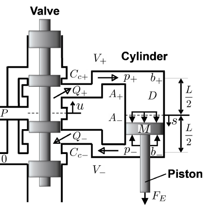
Fig. 1. A hydraulic cylinder and a valve.
2. Preliminary
In this section, we review a nonlinear nominal model of a hydraulic cylinder dynamics and a Casimir function, which is a structural property of mechanical systems coupled with driving systems, such as dynamic actuators or dynamic flexibility.
2.1. Nonlinear Nominal Model 6,7
Figure 1 shows a hydraulic cylinder, pipes, and a valve. We review the nonlinear nominal model in the original representation (e.g., 6,7):
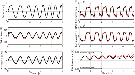
Fig. 2. Experiment result (black) vs. simulation result (red).
2.2. Casimir Function 10
In conventional robotic systems and control, one of the most popular representations is Lagrangian form, which is described by
In the sequel we shall use the port Hamiltonian formulation, which is precisely suited for such systems and allows for use of control inputs that are not generalized forces, and state spaces that are not tangent bundles of some configuration space 11,12. A (standard) port-Hamiltonian form is described by
A Casimir function \(C(x) \in {\mathbf{R}}\) is defined as a solution of the following PDE:
From this definition, if \(u=0\),
The nonlinear nominal model (Eq. \(\eqref{eq:EEQQSS}\)) is equivalent to the state space equation of the following port-Hamiltonian system 13:
Consider system \(\eqref{eq:JTEQ}\). Then there exists a set of a coordinate transformation, an input transformation \(v=g_fu\), and a Hamiltonian replacement, which converts system \(\eqref{eq:JTEQ}\) into the following system 10,14,15
The reduced third order system is just a design model and we need the original fourth order system in the implementation procedure. Please see 10 in detail.
3. Proposed Method
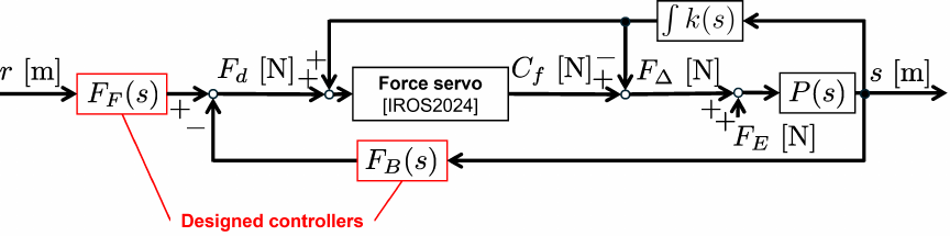
Fig. 3. Block diagram with desired disturbance response model + desired reference response model.
Conventional force servos had the problem of being unable to account for uncertainty in feedback linearization (which partially compensates for terms in the nonlinear nominal model). In contrast, the previously reported force servo 16 automatically corrects feedback linearization taking uncertainty into account. Therefore, assuming a singular perturbation using the previously reported force servo 16,17, the transfer function \(P(s)\) from the differential force \(F_\Delta\) to the piston displacement \(s\) can be represented as:
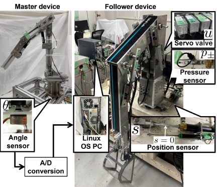
Fig. 4. Experimental setup (left: master device, right: follower device with bucket).
4. Experiment
4.1. Conditions
Figure 4 shows an appearance of the experimental master device and follower device. The experimental setup consists of a vertical and articulated 3-DOF arm, a pump (NDR081-071H-30, 14 L/min, \(P=7\) MPa), a tank (7 L), four pipes (SWP70-6, 1/4 inch), a valve (LSVG-01EH-20-WC-A1-10, gain \(-\)3 dB: 230 Hz, phase \(-\)90°: 270 Hz), two cylinders (asymmetric cylinder (KW1CA30\(\times\)200, \(L = 200\) mm)), a filter (UM-03-20U-1V), and an oil (ISOVG32, 860 kg/m\(^3\), 30\(\pm\)2°C). Table 1 shows the value of the known parameters: the output \(s\) is measured by a potentiometer (LP 100F-C) the output signals \(p_{\pm}\) are measured by a pressure sensor (AP-15S), and the control input \(u\) are measured by the LVDT (1 mm/1.4 V). The output signal of \(s\) is subjected to low-pass-filter \({1}/{(9\times 10^{-3}s+1)^2}\). These output and input signals are detected by an AD converter (PCI-3155, 16 bit) and recorded by a control PC (LX7700, Linux, 2.53 GHz) 19 by a sampling time 1 ms). The control input is applied via a DA converter (PCI-3325, 12 bit).
In addition, the output signal \(\theta\) of the master device is measured by a potentiometer (Midori Precision, CP-20H). The output signal is detected by the same AD converter and recorded by the same control PC. The master device has 3-DOF, and the proposed controller was implemented on its 0th (swing) joint. In all experiments, the bases of both the master and follower manipulators were placed on level surfaces.
Figure 5 shows the U-shaped concrete flume (left) and the bucket (right) used in the experiment. There are two cases: a non-curved case and a curved case. In both cases, three U-shaped concrete flumes are used: the longest U-shaped concrete flume (1.00 m, 0.26 m, 0.20 m), the middle U-shaped flume (0.50 m, 0.26 m, 0.20 m), and the shortest flume (0.25 m, 0.26 m, 0.20 m). In the curved case, they do not share a centerline: the angle between the shortest U-shaped flumes is 20°. For master device, the 0th joint is denoted by \(\theta_0\) [rad], and the 1st and 2nd joint are denoted by \(\theta_1\) and \(\theta_2\) [rad]. Each triangle length in Fig. 6 is given as: (\(\ell_{a0}\), \(\ell_{b0}\), \(\ell_{c0}\)) \(=\) (0.160 m, 0.265 m, 0.370 m) and each triangle length in Fig. 7 is given as: (\(\ell_{a1}\), \(\ell_{b1}\), \(\ell_{c1}\)) = (0.110 m, 0.315 m, 0.283 m), (\(\ell_{a2}\), \(\ell_{b2}\), \(\ell_{c2}\)) \(=\) (0.100 m, 0.315 m, 0.295 m), respectively.
Table 1. Physical parameters of the hydraulic arm.

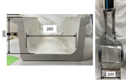
Fig. 5. U-shaped concrete flume (left) and bucket (right). 3 types of U-shaped concrete flume with identical cross-sectional dimensions but different lengths are used. The bucket is attached to the end of the follower device.
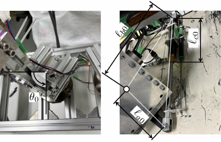
Fig. 6. Master device and follower device (the rotational joint around the horizontal axes).
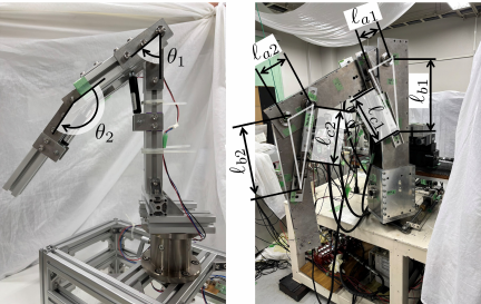
Fig. 7. Rotation of the master device and follower device’s 2 axes.
Table 2. Controller parameters.

In the paper, we assume that the driving force \(A_+p_+ - A_-p_-\) is obtained from the pressure measurement only. The reference input \(r\) [m] is derived by converting the angle \(\theta_0\) of the master device based on the standard cosine theorem. The designed controllers consist of a feedforward controller \(F_F(s)\) that receives the reference input \(r\) [m] and a feedback controller \(F_B(s)\) that takes the output piston displacement \(s\) [m] as the input.
Table 1 shows the value of the parameters. The nonlinear nominal numerical simulator is constructed with the physical parameters (1.7 GHz, 32.0 GB, 64 bit, MATLAB R2015a, Simulink 8.5, ode113 (Adams), maximum step size \(T_\mathrm{max} = 1\), minimum step size \(T_\mathrm{min} = 1\)). Table 2 shows the value of the controller parameters.
4.2. Results
Figures 8 and 9 show the appearance of the preliminary laboratory test of U-shaped concrete flume contact using the master–follower system (non-curved section). Fig. 10 shows the time responses of PID control and the proposed control for piston displacement \(s\) (non-curved section). The proposed method applied the proposed control to the swing joint (0th joint) only, while it applied PID control to the other two joints (1st and 2nd joints). The conventional method applied PID control to all three joints (0th, 1st, and 2nd). In both cases, the bucket did not contact the U-shaped concrete flume and there was no damage.
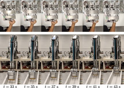
Fig. 8. Preliminary experiment using a master–follower system with a U-shaped concrete flume based on the conventional methods (non-curved section).
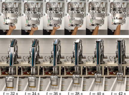
Fig. 9. Preliminary experiment using a master–follower system with U-shaped concrete flume based on the proposed method (non-curved section).
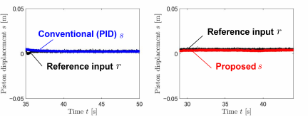
Fig. 10. Time response of piston displacement \(s\) around the swing axis in a non-curved U-shaped concrete flume (PID vs. proposed method). Blue dots indicate the conventional method (PID control), red dots indicate the proposed method.
Figures 11 and 12 shows a preliminary laboratory test of U-shaped concrete flume contact using a master–follower system (curved section). In the conventional method, the bucket damaged the U-shaped flume. On the other hand, in the proposed method, the bucket did not damage the U-shaped flume. Fig. 13 shows the time responses of the piston displacement \(s\) (curved section) by PID control and the proposed control.
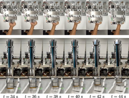
Fig. 11. Preliminary experiment using a master–follower system with U-shaped concrete flume based on the conventional method (curved section).
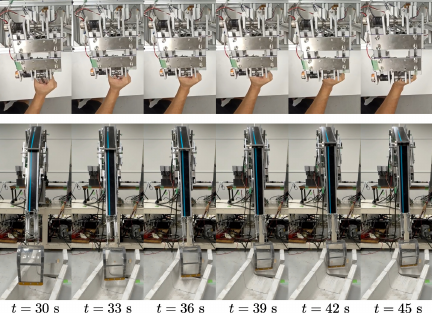
Fig. 12. Preliminary experiment using a master–follower system with U-shaped concrete flume based on the proposed method (curved section).
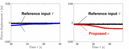
Fig. 13. Time response of the piston displacement \(s\) (non-curved section) by PID control and the proposed control.
Figure 14 shows the bode plots for the closed-loop system from the external force \(F_E\) to the piston displacement \(s\) and also for the closed-loop system from the reference input \(r\) to the piston displacement \(s\). The closed-loop system from reference input to output piston displacement \(s\) followed the reference response model up to 0.1 Hz. Meanwhile, the closed-loop system from the external force \(F_E\) to the piston displacement \(s\) followed the disturbance response model in the frequency ranges 0.2–2.0 Hz.
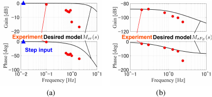
Fig. 14. Bode plots of the reference response model \(M_{sr}(s)\) and the closed-loop system from the reference input \(r\) to the output piston displacement \(s\), as well as those of the disturbance response model \(M_{sF_E}(s)\) and the closed-loop system from the external force \(F_E\) to the output piston displacement \(s\). Black lines indicate the desired models, and red dots indicate the experiments (sinusoidal test). Blue triangles also indicate the experiments (step test).
4.3. Discussion
As shown in Figs. 11–13, the conventional method performs position control only. Even when the bucket contacts the U-shaped concrete flume and the piston displacement changes, it continues to prioritize tracking the reference input and drives the displacement error to zero. Consequently, during the contact, the bucket cannot follow the flume geometry, which is believed to have caused damage to the U-shaped concrete flume. In contrast, the proposed method allows the piston displacement to change almost proportionally to the contact force during the contact, enabling the bucket to follow the flume shape. As a result, no damage was observed. Fig. 14 shows the corresponding bode plots. It is observed that the reference response model \(M_{sr}(s)\) and the disturbance response model \(M_{sF_E}(s)\) were designed well simultaneously especially in the low-frequency range.
5. Conclusion
This paper discusses the effectiveness of a controller that simultaneously satisfies force-sensorless, impedance control and position orientation tracking control using ready-made components. First, we reviewed hydraulic cylinder dynamics with nonlinear pressure dynamics. Second, we designed a controller that applies existing methods so that assuming a situation where unknown external forces act, the controller simultaneously satisfies both the reference response model and the disturbance response model Third, we discussed preliminary indoor experiments simulating waterway cleaning. No custom-made cylinders, valves, pipes are used in our experiments. Future work involves converting the control to the time domain for nonlinear control.
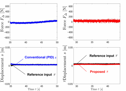
Fig. 15. Time response of the piston displacement \(s\) and the differential force \(F_\Delta\) (non-curved section) by PID control and the proposed control.
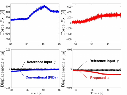
Fig. 16. Time response of the piston displacement \(s\) and the differential force \(F_\Delta\) (curved section) by PID control and the proposed control.
Appendix A. Experimental Results
The more details of the experimental results are given. Fig. 15 compares the time responses of piston displacement \(s\) and differential force \(F_\Delta\) (non-curved section) for PID control and the proposed control method. Fig. 16 compares the time responses of piston displacement \(s\) and differential force \(F_\Delta\) (curved section) for PID control and the proposed control method.
Acknowledgments
We express our gratitude to Ryo Arai, Yuki Imai, Ryota Kasei, and Minoru Hiraoka for their valuable technical discussions. We thank Seiko Precision Inc. and IMW Hose Supply for their supports. The authors would like to thank the reviewers for their valuable comments.
- [1] A. D. Terenteva, “PID-control systems on single-bucket excavators during construction work in urban environments,” Int. J. of Mechanical Engineering and Robotics Research, Vol.10, No.5, pp. 224-229, 2021. https://doi.org/10.18178/ijmerr.10.5.224-229
- [2] D. Won and W. Kim, “Disturbance observer based backstepping for position control of electro-hydraulic systems,” Int. J. of Control, Automation and Systems, Vol.13, No.2, pp. 488-493, 2015. https://doi.org/10.1007/s12555-013-0396-y
- [3] T. Noritsugu and M. Takaiwa, “Impedance control of pneumatic servo system using disturbance observer,” Trans. of the Society of Instrument and Control Engineers, Vol.30, No.6, pp. 677-684, 1994 (in Japanese). https://doi.org/10.9746/sicetr1965.30.677
- [4] F. Abry, X. Brun, S. Sesmat, É. Bideaux, and C. Ducat, “Electropneumatic cylinder backstepping position controller design with real-time closed-loop stiffness and damping tuning,” IEEE Trans. on Control Systems Technology, Vol.24, No.2, pp. 541-552, 2016. https://doi.org/10.1109/TCST.2015.2460692
- [5] Q. P. Ha, Q. H. Nguyen, D. C. Rye, and H. F. Durrant-Whyte, “Impedance control of a hydraulically actuated robotic excavator,” Automation in Construction, Vol.9, Nos.5-6, pp. 421-435, 2000. https://doi.org/10.1016/S0926-5805(00)00056-X.
- [6] S. Sakai and S. Stramigioli, “Visualization of hydraulic cylinder dynamics by a structure preserving nondimensionalization,” IEEE/ASME Trans. on Mechatoronics, Vol.23, No.5, pp. 2196-2206, 2018. https://doi.org/10.1109/TMECH.2018.2854751
- [7] J. Mattila, J. Koivumäki, D. G. Caldwell, and C. Semini, “A survey on control of hydraulic robotic manipulators with projection to future trends,” IEEE/ASME Trans. on Mechatronics, Vol.22, No.2, pp. 669-680, 2017. https://doi.org/10.1109/TMECH.2017.2668604
- [8] H. Merritt, “Hydraulic control systems,” John Willey and Sons, 1967.
- [9] Q. Zhang, “Basics of hydraulic systems,” Taylor & Francis, 2008. https://doi.org/10.1201/9781420071023
- [10] S. Sakai, “Fast computation by simplifications of a class of hydro-mechanical systems,” IFAC Proc. Volumes, Vol.45, No.19, pp. 7-12, 2012. https://doi.org/10.3182/20120829-3-IT-4022.00006
- [11] A. van der Schaft and B. M. Maschke, “The Hamiltonian formulation of energy conserving physical systems with external ports,” Archiv für Elektronik und Übertragungstechnik, Vol.49, pp. 362-371, 1995.
- [12] A. van der Schaft, “L2-Gain and Passivity Techniques in Nonlinear Control, 2nd ed.,” Springer, 2017. https://doi.org/10.1007/978-3-319-49992-5
- [13] A. Kugi and W. Kemmetmuller, “New Energy-based Nonlinear Controller for Hydraulic Piston Actuators,” European J. of Control, Vol.10, No.2, pp. 163-173, 2004. https://doi.org/10.3166/ejc.10.163-173
- [14] S. Sakai, M. Obara, and K. Chikazawa, “Parameter identification via nominal integrator of hydraulic cylinder dynamics,” IFAC-PapersOnLine, Vol.54, No.14, pp. 78-83, 2021. https://doi.org/10.1016/j.ifacol.2021.10.332
- [15] S. Sakai, “Further result on the fast computation of a class of hydro-mechanical systems,” Proc. of IFAC Workshop on Lagrangian and Hamiltonian Methods for Nonlinear Control, 2018.
- [16] R. Arai, S. Sakai, and K. Ono, “Response improvement of hydraulic robotic joints via a force servo and inverted pendulum demo,” Proc. of IEEE/RSJ Int. Conf. on Intelligent Robots and Systems (IROS), pp. 761-766, 2024. https://doi.org/10.1109/IROS58592.2024.10802664
- [17] R. Arai and S. Sakai, “Model validation using ready-made components toward flexible hydraulic joints,” J. Robot. Mechatron., Vol.37, No.1, pp. 76-85, 2025. https://doi.org/10.20965/jrm.2025.p0076
- [18] K. Kumabe, S. Sakai, R. Arai, and R. Umemoto, “Master-follower peg-in-hole local experiment using nonlinear hydraulic arms,” Proc. of the JFPS Int. Symposium on Fluid Power, Article No.P1-12, 2024.
- [19] S. Sakai, M.Iida, K. Osuka, and M. Umeda, “Design and control of a heavy material handling manipulator for agricultural robots,” Autonomous Robots, Vol.25, pp. 189-204, 2008. https://doi.org/10.1007/s10514-008-9090-y
This article is published under a Creative Commons Attribution-NoDerivatives 4.0 Internationa License.