Paper:
Transition Long-Period Map for the National Structural Code of the Philippines
Rhommel N. Grutas†
 , Koreen G. Dorado
, Justine Anne O. Duka
, Miguel Antonio T. Magandi
, Rizza Micaela S. Padre
, John Edward A. Nachor
, Nicole P. Tenorio
, Nicole Ann B. Bersabe
, and Teresito C. Bacolcol
, Koreen G. Dorado
, Justine Anne O. Duka
, Miguel Antonio T. Magandi
, Rizza Micaela S. Padre
, John Edward A. Nachor
, Nicole P. Tenorio
, Nicole Ann B. Bersabe
, and Teresito C. Bacolcol
Department of Science and Technology, Philippine Institute of Volcanology and Seismology (DOST-PHIVOLCS)
PHIVOLCS Building, C.P. Garcia Avenue, UP Campus, Diliman, Quezon City 1101, Philippines
†Corresponding author

The National Structural Code of the Philippines is set to be updated to align with international standards through the adoption of the Minimum Design Loads and Associated Criteria for Buildings and Other Structures of the American Society of Civil Engineers 7-05. This development introduces new key parameters in the ground motion section, specifically the transition long-period (TL), which is essential for the long-period structure seismic design. To accurately represent ground motion at periods greater than 4 s, which are critical for the design of long-period structures, such as high-rise buildings, and to determine the TL values specific to the Philippines, data derived from the Seismic Hazard Assessment for the Design Earthquake of the Philippines Project, implemented by the Philippine Institute of Volcanology and Seismology, were utilized. Using this dataset, modal magnitude (Md) maps were developed through the disaggregation of the 2% probability of exceedance in 50 years for spectral acceleration (Sa) at T=2 seconds, which were then correlated with the corresponding corner period (Tc) values. The seismic source models were subdivided into fault, subduction, and area sources. Results indicate that, in areas located near fault sources, magnitudes are predominantly influenced by the crustal earthquake generators. However, subduction sources tend to dominate the earthquake magnitudes in regions farther from the crustal fault systems.
1. Introduction
As one of the fastest-growing urban populations in Asia, rapid urbanization in the Philippines has led to the densification of major cities, with the Metro Manila urban agglomeration as one of the densest in the country 1. To accommodate the increased concentration of people and economic activities in urban areas, cities have undergone significant structural transformations that can be demonstrated by the prevalence of high-rise residential and commercial buildings, as well as other mixed-use, high-density structures found in most metropolitan areas in the country. These vertical structures require additional considerations in terms of safety and design standards to ensure stability against increased sway and vibrations during earthquakes/ground motion events. Thus, a more specific approach is necessary to precisely measure ground motion to improve the safety of urban environments. The resilience of these structures mainly relies on their design standards, quality of materials, workmanship, and most importantly, the seismicity of the region the structures reside. The active seismic setting of the Philippines magnifies the critical need to account for dynamic forces, such as ground motion, that may impact structures and lead to damage. The Philippines is situated in a complex tectonic setting with various subduction complexes surrounding the archipelago on the eastern and western sides and active faults, including a prominent left-lateral strike-slip fault transecting across the archipelago called the Philippine Fault 2. The delineation of the Philippine Fault and the distribution of the other earthquake generators in the Philippines are shown in Fig. 1. These features make the country highly vulnerable to frequent and destructive earthquakes such as the \(M_s\) 7.2 2013 Bohol earthquake, the \(M_s\) 6.7 2017 Surigao earthquake, \(M_s\) 6.5 2017 Leyte earthquake, the 2019 Cotabato earthquake series with magnitudes ranging from 6.1 to 6.6, and the \(M_{\textrm{w}}\) 7.0 2022 Northwestern Luzon earthquake. These earthquake events have resulted in numerous casualties, extensive structural damage, and devastating impacts on local livelihoods in the affected areas.
Basic forms of disaster risk reduction and management efforts necessitate accurate assessments of seismic hazards, particularly for ground motion in areas in close proximity to major active faults and subduction zones. Ground motion is usually established using seismic hazard analysis, either by accounting historical maximum ground motion with a certain scenario as deterministic, or through accounting for the likelihood of ground motion from different sources over a period of time in a probabilistic approach.
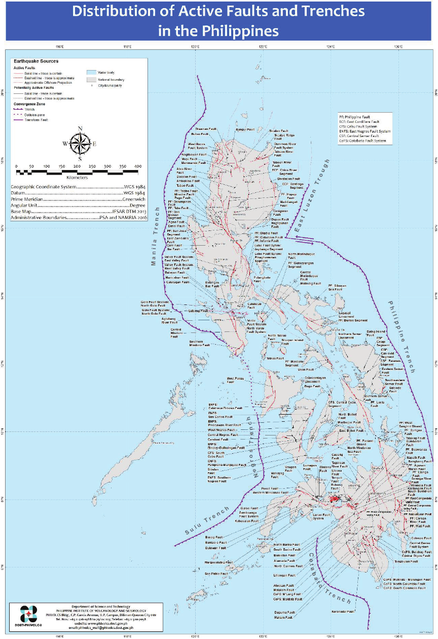
Fig. 1. Distribution of earthquake generators in the Philippines.
Given that the Philippines is located in a seismically active region, comprehensive analyses are necessary to address uncertainties related to potential earthquakes thereby enhancing the reliability of seismic hazard assessments. In the field of structural engineering, recent advancements have contributed to the development of the concept of the maximum considered earthquake (MCE), which represents the ground motion a structure must be able to withstand, as defined by the standards set forth by the American Society of Civil Engineers (ASCE) in its publication of the ASCE 7 or the Minimum Design Loads for Buildings and Other Structures 3. The MCE corresponds to a 2% probability of exceedance in 50 years, equivalent to a return period of approximately 2,500 years. This concept is essential for creating seismic hazard maps and serves as a reference for building codes to ensure that structures can withstand such events.
The MCE serves as a standard for ensuring safety, particularly in the design of most buildings where resilience to seismic events is crucial. However, models such as the MCE may not be enough to represent ground motion in high-rise structures, as most of these models fail to account for the oscillations tall buildings experience as the result of their low frequency, long-period response to seismic forces. Crouse et al. 4 specify that most ground motion models do not consider seismic response periods greater than five seconds. To account for the long-period for high-rise structures, the Building Seismic Safety Council developed a method for estimating and mapping out the so-called transition long-period values within a region.
Transition long-period (\(T_L\)) is an important parameter that is currently included in the American Society of Civil Engineers (ASCE) 7-05 structural standards. It was first introduced in the FEMA 450-1/2003 as part of the National Earthquake Hazard Reduction Program (NEHRP) Recommended Provisions for Seismic Regulations for New Buildings and Other Structures and has not been thoroughly revisited in subsequent standards, despite its importance in accurately assessing seismic demands on structures 5. The \(T_L\) parameter plays a crucial role in the dynamic analysis of high-rise buildings due to the structure’s height and associated structural periods. It marks the transition between the constant velocity and constant displacement segments of the design response spectrum. By incorporating the \(T_L\) parameter in the design process, the design of high structures can be refined and the overall resilience of the structure to earthquake-induced forces can be improved.
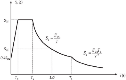
Fig. 2. Design response spectrum as specified in ASCE 7-05: Minimum Design Loads for Buildings and Other Structures.
The design response spectrum (DRS) is an essential tool commonly used by engineers as a means of comprehending the structural dynamics of a building. This concept helps with a structure’s design by creating a graphical representation that can determine the behavior of the structure under particular ground motion and period conditions, making it a fundamental part of constructing earthquake-resilient structures. The ideal DRS graph is composed of three spectral segments: constant acceleration, constant velocity, and constant displacement, with the \(T_L\) parameter separating the constant velocity and constant displacement sectors. The DRS is typically divided into three segments: the short-period range, the transition range, and the long-period range. In the short-period range, structures experience higher accelerations, while in the long-period range, the spectral demands are often lower, which can lead to underestimations of the seismic response for structures designed for longer periods 6. Fig. 2 displays the two-period DRS as shown in ASCE 7-05. Understanding the overall two-period design response spectrum is crucial as the National Structural Code of the Philippines is set to update from the Uniform Building Code of 1997 7 to the ASCE 7-05.
The code calculates the spectral acceleration for specified structural periods given by the equations:
-
1)
For periods less than \(T_o\) (\(T<T_o\)), \(S_a\) shall be computed by Eq. \(\eqref{eq:1a}\):
\begin{equation} \label{eq:1a} S_a=S_{\textit{DS}}\left(0.4+0.6\dfrac{T}{T_o}\right).\tag{1a} \end{equation} -
2)
For periods greater than or equal to \(T_o\) and less than or equal to \(T_s\) (\(T_o\le T\le T_s\)), \(S_a\) shall be computed by Eq. \(\eqref{eq:1.2}\):
\begin{equation} \label{eq:1.2} S_a=S_{\textit{DS}}.\tag{1b} \end{equation} -
3)
For periods greater than \(T_S\) and less than or equal to \(T_L\) (\(T_s<T\le T_L\)), \(S_a\) shall be computed by Eq. \(\eqref{eq:1.3}\):
\begin{equation} \label{eq:1.3} S_a=\dfrac{S_{D1}}{T}.\tag{1c} \end{equation} -
4)
For periods greater than \(T_L\) (\(T>T_L\)), \(S_a\) shall be computed by Eq. \(\eqref{eq:1.4}\):
\begin{equation} \label{eq:1.4} S_a=\dfrac{S_{D1}\times T_L}{T^2},\tag{1d} \end{equation}where \(S_{\textit{DS}}\) is equal to \((2/3)S_{\textit{MS}}\) and \(S_{D1}\) is equal to \((2/3)S_{M1}\). The values of \(S_{\textit{MS}}\) and \(S_{M1}\) are calculated using the following formulae:\begin{align} \label{eq:2} &S_{\textit{MS}}=F_a\times S_s,\tag{2}\\ \end{align}\begin{align} &S_{M1}=F_v\times S_1.\label{eq:3}\tag{3} \end{align}
In Eqs. \(\eqref{eq:2}\) and \(\eqref{eq:3}\), \(F_a\) and \(F_v\) represent the site amplification factor, while \(S_s\) and \(S_1\) are the short-period spectral acceleration and 1-second spectral acceleration from the MCE map.
Recent studies have highlighted the necessity of incorporating \(T_L\) into seismic design frameworks to ensure that structures can adequately withstand long-period ground motion. For example, the empirical evaluation of spectral ordinates indicates that the displacement response spectrum is often more relevant for long-period structures than the acceleration response spectrum 6. This is important for ensuring that design spectra accurately reflect the seismic demands imposed on structures, particularly in regions prone to long-period ground motion 8.
Given that the Philippines is located in a seismically active region, and it’s cities becoming more urbanized, and populated with skyscrapers and tall buildings, a transition long-period map is proposed to enhance the accuracy of ground motion estimates, thereby producing more reliable seismic design for high-rise buildings.
2. Transition Long-Period
The transition long-period (\(T_L\)) is the point in which the earthquake response spectrum shifts from constant velocity to constant displacement. It is crucial for seismic design of the the high-rise buildings, as it affects how these structures respond to ground motions. Precise, site-specific \(T_L\) values, derived from a refined seismic hazard repository, enable more reliable and robust designs. In the current structural code used in the Philippines, ground motion is often characterized through both \(S_{\textit{MS}}\) and \(S_{M1}\), neither of which take into account ground motions at \(T>4\) seconds.
The procedure and rationale for developing the TL maps, as detailed in Crouse et al. 4, involved two main steps: first, establishing a relationship between \(T_L\) and earthquake magnitude; second, mapping the modal magnitude from the disaggregation of the USGS 2% in 50-year ground motion hazard at a 2-second period. The resulting \(T_L\) maps, which combine these steps, define the point in the design response spectrum where the shape transitions from constant velocity (\(1/T\)) to constant displacement (\(1/T^2\)).
3. Methodology
To determine the \(T_L\) values in the Philippines, modal magnitude maps were constructed by disaggregating the 2% in 50-year hazard (return period of 2,475 years) for \(S_a\) (\(T=2\) s.), i.e., the 5% damped response spectral acceleration at a 2 s oscillator period. The \(T_L\) parameter plays a vital role in the two-period design response spectra as it affects both the constant spectral displacement and constant spectral velocity segments. However, it is often neglected in constructing design response spectra for conservative purposes 9.
3.1. Probabilistic Seismic Hazard Assessment
Probabilistic seismic hazard assessment (PSHA) is a methodology used to estimate seismic hazard by considering various sources of uncertainty 10. Earthquake occurrences are considered random processes, modelled using probability distributions for location, magnitude, and ground motion intensity. Modelling involves assessing the likelihood of different levels of ground shaking occurring at a specific location within a given timeframe 11. PSHA typically provides estimates of parameters such as peak ground acceleration (PGA) and spectral acceleration (\(S_a\)) to quantify the seismic hazard at a particular site 12. This approach allows for the consideration of uncertainties related to seismic hazard, making it a more comprehensive framework in contrast to deterministic methods 13.
Moreover, Kramer 14 presents the systematic process of PSHA in assessing seismic risks that involves four main steps. First, it is necessary to identify and characterize each earthquake source zone by assigning a uniform probability distribution to potential rupture locations. Unlike deterministic seismic hazard assessment (DSHA), which only considers the closest points, PSHA treats all locations within a source as equally likely. Second, a recurrence relationship is established for each source zone to characterize the temporal distribution and frequency of earthquakes, and PSHA analyzes a broader range of potential earthquake sizes. Next, the ground motion at the site is determined by considering the range of possible earthquake magnitudes and locations within each source zone, along with the associated predictive uncertainties. Lastly, all uncertainties related to earthquake location, size, and ground motion are integrated to compute the probability that a specific ground motion will exceed a defined threshold.
The OpenQuake engine, an open-source software package developed by the Global Earthquake Model (GEM) 15,16, was utilized in conducting PSHA. Seismic source models mainly consist of seismic source and ground motion characterizations and the uncertainties both components. From these input files, the amount of ground shaking an earthquake may cause can be assessed.
3.1.1. Seismic Source Model
Identifying earthquake generators is crucial in seismic hazard analysis to assess the potential impact of earthquakes that may originate from a specific source. Seismic source characterization includes the description of possible seismic generators and the occurrence of earthquakes per source.
3.1.1.1. Earthquake Catalogs
A compilation of different local and global earthquake catalogs was used to create a comprehensive unified earthquake catalog for the Philippines. Earthquake events from the Department of Science and Technology, Philippine Institute of Volcanology and Seismology (DOST-PHIVOLCS) and GEM of the International Seismological Centre (ISC) were used to create a comprehensive earthquake catalog of the Philippines along with historical earthquake data 17,18 dating from 1608 to 2022 with moment magnitudes ranging from 5.0 to 8.3. The selected range of high magnitudes focuses on the most relevant data that can cause significant ground shaking or potential structural damages.
The compiled earthquake catalogs were preprocessed through data cleaning and formatting of the collected earthquake events. This included ensuring a uniform attribute format across all events, eliminating redundant entries for the same event, removing entries with incomplete times and dates and misleading data such as events with earthquake magnitude of zero. Pre-processing was done through database management systems with Python scripting.
As data from both global and local catalogs were compiled, homogenization, i.e., ensuring a uniform unit for measuring earthquake magnitude, was necessary. Event details from the compiled earthquake catalogs included measures of the surface wave magnitude, \(M_s\), body wave magnitude, \(M_b\), and the local magnitude, \(M_L\), aside from the generally used moment magnitude, \(M_{\textrm{w}}\). Magnitude-homogenization conversions by Scordilis, Lolli et al., and Weatherill et al. 19,20,21 were investigated by the project, to ultimately utilize the conversions by Weatherhill et al. 21 due to similarities of earthquake catalogs used (ISC-GEM and ISC-Reviewed Bulletins), along with the consideration of different local catalogs.
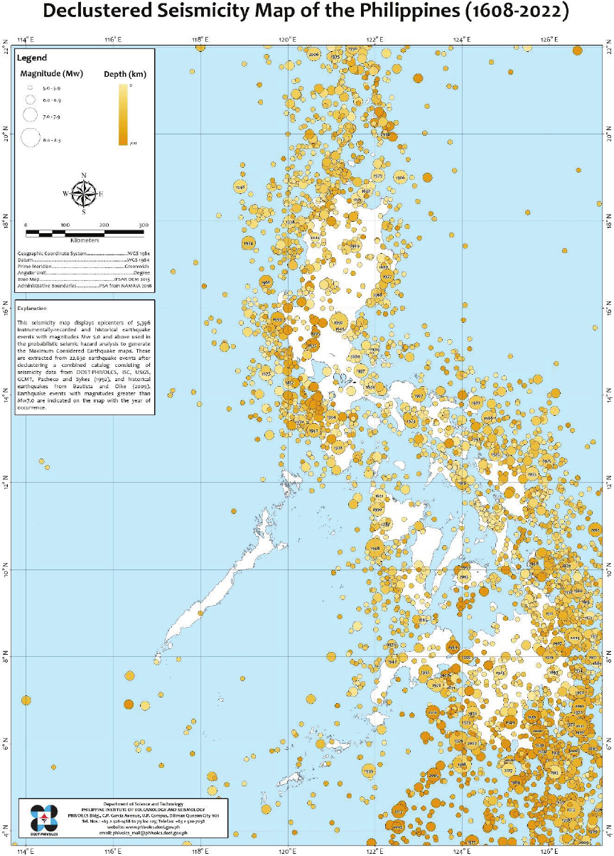
Fig. 3. Distribution of mainshocks in the Philippines ranging from magnitude 5.0 to 8.3.
The homogenized catalog was then declustered to separate mainshocks from foreshocks and aftershocks from the spatiotemporal data of each earthquake event using the Window Method of Gardner and Knopoff 22. This step is necessary to ensure that the events are independent of one another, as foreshocks and aftershocks are temporally and spatially dependent on the mainshock events and are to be removed 23. The events were classified by focal depth into crustal, subduction interface, intraslab, and area sources to precisely characterize seismicity associated with the earthquake generators. Fig. 3 highlights the distribution of the declustered seismicity in the Philippines.
3.1.1.2. Source Model
The seismic sources considered for this study were subdivided into active crustal faults, subduction interface seismicity, and distributed seismicity. These sources were modeled accordingly based on their geometry and kinematics.
The active crustal faults represent the cracks or fractures that are capable of generating earthquakes. The parameters in modeling crustal faults included the fault’s geometry and kinematics, which were derived from DOST-PHIVOLCS’ database. For calculation purposes, the fault data were modified by simplifying the fault traces. A total of 220 crustal faults were delineated. Some known fault parameters, such as the strike, dip, and rake, were assimilated from previous studies 24,25,26,27,28,29,30,31 and through centroid moment tensor (CMT) data 32,33,34. Each fault was modeled as a planar surface extending from the assigned upper seismogenic depth of 5 km down to the lower seismogenic depth of 30 km, oriented along the dip direction with an inclination equal to the fault dip angle.
The subduction sources have been subdivided into two categories, the subduction interface and subduction intraslab, both of which were modeled differently as illustrated in Fig. 4. The subduction interface source refers to the seismicity caused by the trenches surrounding the Philippine archipelago. This source typology includes the Manila Trench, Philippine Trench, Negros Trench, Sulu Trench, Cotabato Trench, and East Luzon Trough. Each interface was subdivided into different segments according to the earthquake source parameters, such as the fault width, dip angle, rake, and amount of slip, set by Salcedo 35. To account for the irregularities of the surface of the interfaces, each segment was modeled as a mesh by indicating the top, intermediate, and bottom edges. The geometries of the subducting slabs were based on the models in Slab2.0 36. The subduction intraslab, differentiated from the subduction interface through depth constraints, refers to sources of much deeper origin, with a depth of 60 km and above. In contrast with the subduction interface sources, not all trench systems in the Philippines have subduction intraslab sources. Some trench systems, such as the East Luzon Trough, Negros Trench, and Sulu Trench, and some segments of the Philippine Trench have not been included due to the limited amount of subduction intraslab-related seismicity. It is also important to note that these omitted trench systems may still constitute potential seismic sources requiring further investigation as additional data become available.
Crustal earthquakes that cannot be attributed to a specific fault as well as trench-related earthquakes were classified as distributed seismicity and modeled as area sources. The area sources were modeled as polygons, grouped solely based on seismicity and tectonic classification.
To simulate the earthquake hazards these sources may pose, the magnitude-frequency distribution (MFD) was calculated using the Gutenberg–Richter relation 37, which represents the overall level of seismic activity and the relative frequency of small earthquakes versus large earthquakes. The Gutenberg–Richter law states that earthquake magnitudes are distributed logarithmically, expressed as
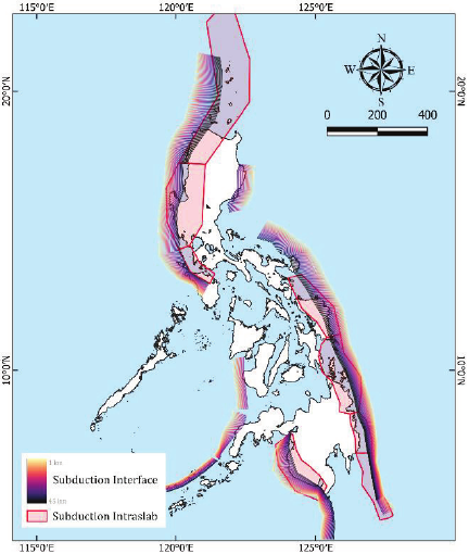
Fig. 4. Seismic source model of the subduction zones in the Philippines.
3.1.2. Ground Motion Models
Ground motion attenuation models or ground motion prediction equations (GMPEs) are empirical equations that forecast ground motion at a particular site based on an earthquake’s magnitude, source-to-site distance, site conditions and occurrence rates. Different GMPEs are developed for different types of source models, as the equations, which are derived from various datasets and methodologies, can produce a wide range of predictions. The selection of specific GMPEs often accommodates the seismic source type, such as shallow crustal faults or subduction zones, to ensure their applicability to a particular tectonic setting like the Philippines.
GMPEs used in the hazard calculation were derived from the latest input model developed by DOST-PHIVOLCS in partnership with the Global Earthquake Model (GEM) 38. The enhanced GMPEs were utilized to represent the minimum, median, and maximum ground motions. For shallow crustal faults, Boore et al. and Chiou and Youngs 39,40 were selected to account for the median ground motion. Boore et al. 39 and its low-Q model, referring to rock quality factors, were used to represent the lower ranges, and Zhao et al. 41 to represent the upper ranges of ground motion. For subduction sources, median ground motion was represented by a more recent GMPE by Parker et al. 42 along with the models by Zhao et al. 41 and Abrahamson et al. 43.
A site model with a 5-km grid and a shear wave velocity of 760 m/s in the upper 30 m (\(V_{s30}\)) was used in the calculation based on the NEHRP recommendations. Table 1 lists the GMPEs utilized in the model with their respective weights. Most of the models are assigned equal weights to account for any epistemic uncertainties in hazard estimation 44. This approach ensures that the hazard estimation is not biased towards a single model. By giving each GMPE equal importance, the overall hazard estimate reflects the full range or average predictions, and all models contribute equally.
Table 1. GMPEs used in the model with their respective weights.

3.2. Disaggregation
Seismic hazard disaggregation is often done to understand the relative contribution to a given frequency of exceedance of each component of the hazard assessment to the overall hazard an area may experience, such as the magnitude \(M\), source-to-site distance \(R\), and the measure of deviation of the ground motion from the mean value, \(\varepsilon\). Through disaggregation, the hazard can be better communicated and the expected ground motion can be further characterized 45.
The disaggregation was done through the disaggregation calculator in the OpenQuake engine. Each component was separated into bins with specific bin widths. For this study, the annular distance was set as 5 km while the magnitude bins were set as 0.5. The maps were developed using sites with grid increments of 5 km in both latitude and longitude.
3.3. Transition Long-Period Parameter
According to Crouse et al. 4, the \(T_L\) parameter can be mapped out through the correlation between earthquake magnitude and \(T_L\). This correlation can be established by analyzing the response spectra of strong motion data of shallow earthquakes and ground motion simulations of large earthquakes. Through the seismic theory 46, the correlation between earthquakes and \(T_L\) can also be identified by investigating the corner period (\(T_c\)) between the intermediate and long-period ground motion.
\(T_c\) serves as the boundary between constant displacement and constant velocity in the Fourier spectrum and can be considered as an approximation for the \(T_L\) parameter. The formula used in correlating \(T_c\) to earthquake magnitude can be seen in Eq. \(\eqref{eq:5}\):
Table 2. Correlation between moment magnitude (\(M_{\textrm{w}}\)) and corner period (\(T_c\)) 4.

4. Results and Discussion
The resulting transition long-period values can be seen in Fig. 5. For areas near fault sources, earthquake magnitudes caused by the local fault dominate. Meanwhile, for areas far from fault sources and near subduction zones, magnitudes caused by the seismicity of subduction zones dominate. This can be observed on the map where some contours almost follow the shape of the fault line. The longest fault in the Philippines, the Philippine Fault, displays a higher value compared to other local faults. This might be due to it being significantly active as this fault accommodates the stress brought upon by the oblique subduction of the Philippine Sea Plate in the Philippine Trench through shear partitioning 2.
The highest \(T_L\) values were observed near the major subduction zones in the Philippines—the westernmost and easternmost sides of the country. The western part of Luzon as well as the southeastern part of the Visayas and Mindanao both display high values of \(T_L\) mainly due to the ongoing subduction in the Manila Trench and the Philippine Trench, respectively.
The Palawan Microcontinental Block (PCB) displays the lowest value for \(T_L\) as this area experiences less seismic activity compared to the Philippine Mobile Belt (PMB), due to its tectonic affinity. Unlike the PMB, the PCB is situated within the more stable Eurasian Plate.
5. Recommendations
The derivation of the \(T_L\) parameter relies on the disaggregated results of the PSHA. As such, the completeness and accuracy of the datasets used in PSHA are necessary considerations to ensure the integrity of the \(T_L\) results. For the compilation of earthquake catalogs, the study used the DOST-PHIVOLCS and ISC catalogs. These catalogs, albeit accurate, can still be refined for completeness and updated as newer events become available. A suitability analysis of the ground motion prediction equations is recommended when selecting of ground motion models to be used for PSHA for further research, as it can significantly influence the \(T_L\) results.
Since the introduction of the \(T_L\) in 2006, other methods for its derivation have also been proposed—may it be through seismological approach 5 or through close examination of the maximum spectral displacement in the design response spectra for considering earthquakes in subduction zones 47. Assadollahi et al. 5 proposed a seismic model for approximating the \(T_L\) values based on Brune’s Seismic Model, incorporating regional stress drop (\(\Delta\sigma\)) and crustal velocity (\(\beta\)) to produce higher and more conservative \(T_L\) estimates. By introducing regional \(T_L\) estimates, this approach allows for smoother variations in \(T_L\) maps, in contrast to Crouse et al. 4, whose methodology results in sharper boundaries due to its reliance solely on modal magnitude. While the proposed model offers regionally tailored \(T_L\) values, its applicability is constrained by data availability, as stress drop and crustal velocity values are not always well-documented or well-constrained, particularly in the regional scales of the Philippines. Additionally, this method has not yet been integrated into the country’s structural code, limiting its immediate adoption in seismic design practice.
Given its established use from ASCE 7-05 through ASCE 7-22, the straightforward methodology of Crouse et al. 4 was adopted in this study to ensure continuity and consistency in seismic design, aligning with the current building codes implemented in the country. Currently, this method provides a more stable and practical approach for estimating \(T_L\) values in the Philippines, as it has been consistently followed in structural codes over the years. Despite not accounting for key seismological complexities, the method of Crouse et al. 4 has proven valuable in offering insights into the \(T_L\) parameter of the DRS. Unlike more contemporary approaches, which incorporate additional regional factors, Crouse et al. 4 relies on modal magnitude. This limitation may lead to the underestimation of \(T_L\) values, particularly in geologically complex regions where seismic wave propagation and attenuation vary significantly.
Nevertheless, the integration of the \(T_L\) parameter into modern building codes represents a significant advancement in structural resilience, ensuring that long-period structures are adequately designed for seismic demands. Furthermore, this incorporation lays the foundation for the development of more refined methodologies that incorporate additional parameters, ultimately leading to regionally tailored \(T_L\) estimates and improved seismic design practices.
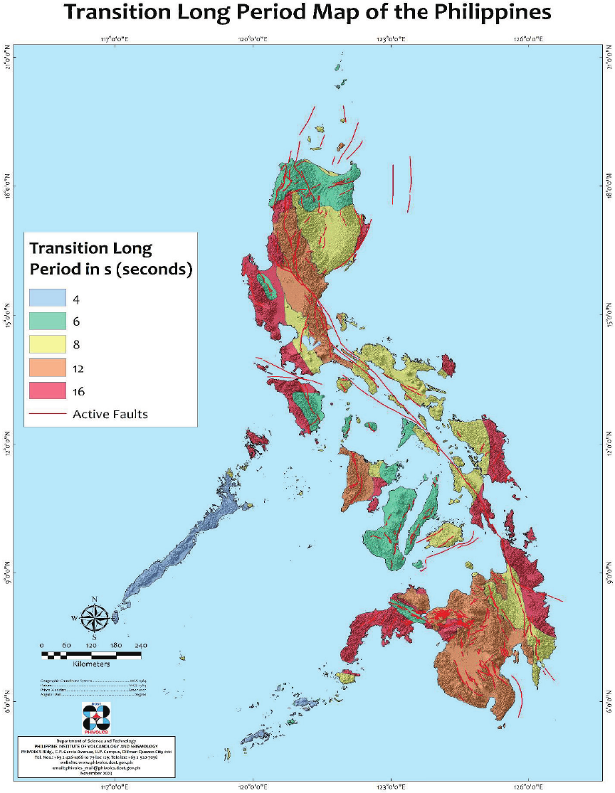
Fig. 5. Derived transition long-period map for the Philippines. The red lines denote the modeled active faults using PHIVOLCS data.
Acknowledgments
This study was developed as part of the outputs of the DOST-GIA Project entitled, “Seismic Hazard Assessment for Design Earthquake of the Philippines,” or the SHADE Project. The authors would like to acknowledge the leadership and support of the Philippine Institute of Volcanology and Seismology (DOST-PHIVOLCS) as the implementing agency, as well as of the Philippine Council for Industry, Energy, and Emerging Technology Research and Development (DOST-PCIEERD) as the monitoring agency for the project.
- [1] World Bank, “Philippines urbanization review: Fostering competitive, sustainable and inclusive cities,” Report No.114088, 1997. https://doi.org/10.1596/27667
- [2] M. A. Aurelio, “Shear partitioning in the Philippines: Constraints from Philippine Fault and global positioning system data,” Island Arc, Vol.9, No.4, pp. 584-597, 2000. https://doi.org/10.1111/j.1440-1738.2000.00304.x
- [3] “Chapter 11: Seismic design criteria,” American Society of Civil Engineers, “Minimum Design Loads for Buildings and Other Structures,” ASCE/SEI 7-05, pp. 115-116, 2006.
- [4] C. Crouse, E. V. Leyendecker, P. G. Somerville, M. Power, and W. J. Silva, “Development of seismic ground-motion criteria for the ASCE 7 standard,” 8th US National Conf. on Earthquake Engineering 2006, pp. 46-53, 2006.
- [5] C. Assadollahi, S. Pezeshk, and K. Campbell, “A seismological method for estimating the long-period transition period TL in the seismic building code,” Earthquake Spectra, Vol.39, No.2, pp. 1037-1057, 2023. https://doi.org/10.1177/87552930231153673
- [6] Y. Chen, L. Xu, X. Zhu, and H. Liu, “A multi-objective ground motion selection approach matching the acceleration and displacement response spectra,” Sustainability, Vol.10, Issue 12, Article No.4659, 2018. https://doi.org/10.3390/su10124659
- [7] “Uniform building code,” Int. Conf. of Building Officials, 1997.
- [8] I. Takewaki, K. Fujita, and S. Yoshitomi, “Uncertainties in long-period ground motion and its impact on building structural design: case study of the 2011 Tohoku (Japan) earthquake,” Engineering Structures, Vol.49, pp. 119-134, 2013. https://doi.org/10.1016/j.engstruct.2012.10.038
- [9] J. J. Bommer, A. S. Elnashai, and A. G. Weir, “Compatible acceleration and displacement spectra for seismic design codes,” Proc. of the 12th World Conf. on Earthquake Engineering, Vol.8, Article No.0207, 2000.
- [10] C. A. Cornell, “Engineering seismic risk analysis,” Bulletin of the Seismological Society of America, Vol.58, No.5, pp. 1583-1606, 1968.
- [11] K. Vipin, P. Anbazhagan, and T. Sitharam, “Estimation of peak ground acceleration and spectral acceleration for South India with local site effects: Probabilistic approach,” Natural Hazards and Earth System Science, Vol.9, Issue 3, pp. 865-878, 2009. https://doi.org/10.5194/nhess-9-865-2009
- [12] P. Anbazhagan, J. Vinod, and T. Sitharam, “Probabilistic seismic hazard analysis for Bangalore,” Natural Hazards, Vol.48, No.2, pp. 145-166, 2008. https://doi.org/10.1007/s11069-008-9253-3
- [13] N. Jayaram and J. Baker, “Efficient sampling and data reduction techniques for probabilistic seismic lifeline risk assessment,” Earthquake Engineering & Structural Dynamics, Vol.39, No.10, pp. 1109-1131, 2010. https://doi.org/10.1002/eqe.988
- [14] S. L. Kramer, “Geotechnical Earthquake Engineering, Chapter 4, Section 4,” Prentice Hall, pp. 117-137, 1996.
- [15] M. Pagani, D. Monelli, G. Weatherill, L. Danciu, H. Crowley, V. Silva, P. Henshaw, L. Butler, M. Nastasi, L. Panzeri, M. Simionato, and D. Vigano, “OpenQuake engine: An open hazard (and risk) software for the global earthquake model,” Seismological Research Letters, Vol.85, No.3, pp. 692-702, 2014. https://doi.org/10.1785/0220130087
- [16] V. Silva, H. Crowley, M. Pagani, D. Monelli, and R. Pinho, “Development of the OpenQuake engine, the Global Earthquake Model’s open-source software for seismic risk assessment,” Natural Hazards, Vol.72, pp. 1409-1427, 2014. https://doi.org/10.1007/s11069-013-0618-x
- [17] J. F. Pacheco and L. R. Sykes, “Seismic moment catalog of large shallow earthquakes, 1900 to 1989,” Bulletin of the Seismological Society of America, Vol.82, No.3, pp. 1306-1349, 1992. https://doi.org/10.1785/BSSA0820031306
- [18] M. L. Bautista and K. Oike, “Estimation of the magnitudes and epicenters of Philippine historical earthquakes,” Tectonophysics, Vol.317, Nos.1-2, pp. 137-169, 2000. https://doi.org/10.1016/S0040-1951(99)00272-3
- [19] E. M. Scordilis, “Empirical global relations converting MS and mb to moment magnitude,” J. of Seismology, Vol.10, No.2, pp. 225-236, 2006. https://doi.org/10.1007/s10950-006-9012-4
- [20] B. Lolli, P. Gasperini, and G. Vannucci, “Empirical conversion between teleseismic magnitudes (mb and Ms) and moment magnitude (Mw) at the Global, Euro-Mediterranean and Italian scale,” Geophysical J. Int., Vol.199, No.2, pp. 805-828, 2014. https://doi.org/10.1093/gji/ggu264
- [21] G. A. Weatherill, M. Pagani, and J. Garcia, “Exploring earthquake databases for the creation of magnitude-homogeneous catalogues: Tools for application on a regional and global scale,” Geophysical J. Int., Vol.206, Issue 3, pp. 1652-1676, 2016. https://doi.org/10.1093/gji/ggw232
- [22] J. K. Gardner and L. Knopoff, “Is the sequence of earthquakes in Southern California, with aftershocks removed, Poissonian?” Bulletin of the Seismological Society of America, Vol.64, pp. 1363-1367, 1974. https://doi.org/10.1785/BSSA0640051363
- [23] O. Boyd, “A visitation of earthquake catalog declustering,” [Presentation slides], U.S. Geological Survey, USGS Seismic Hazard Workshop for CEUS Sources 2012, pp. 1-6, 2012.
- [24] R. E. Rimando and P. L. Knuepfer, “Neotectonics of the Marikina Valley fault system (MVFS) and tectonic framework of structures in northern and central Luzon, Philippines,” Tectonophysics, Vol.415, Nos.1-4, pp. 17-38, 2006. https://doi.org/10.1016/j.tecto.2005.11.009
- [25] H. Tsutsumi and J. S. Perez, “Large-scale active fault map of the Philippine fault based on aerial photograph interpretation,” Active Fault Research, Vol.2013, No.39, pp. 29-37, 2013. https://doi.org/10.11462/afr.2013.39_29
- [26] J. Perez, H. Tsutsumi, M. Cahulogan, D. Cabanlit, M. Abigania, and T. Nakata, “Fault distribution, segmentation and earthquake generation potential of the Philippine fault in eastern Mindanao, Philippines,” J. Disaster Res., Vol.10, No.1, pp. 74-82, 2015. https://doi.org/10.20965/jdr.2015.p0074
- [27] H. Tsutsumi, J. Perez, J. Marjes, K. Papiona, and N. Ramos, “Coseismic displacement and recurrence interval of the 1973 Ragay Gulf earthquake, southern Luzon, Philippines,” J. Disaster Res., Vol.10, No.1, pp. 83-90, 2015. https://doi.org/10.20965/jdr.2015.p0083
- [28] R. E. Rimando and J. M. Rimando, “Morphotectonic kinematic indicators along the Vigan-Aggao Fault: The western deformation front of the Philippine Fault Zone in Northern Luzon, the Philippines,” Geosciences, Vol.10, Issue 2, Article No.83, 2020. https://doi.org/10.3390/geosciences10020083
- [29] R. E. Rimando, J. M. Rimando, and R. B. Lim, “Complex shear partitioning involving the 6 February 2012 Mw 6.7 Negros Earthquake ground rupture in central Philippines,” Geosciences, Vol.10, Issue 11, Article No.460, 2020. https://doi.org/10.3390/geosciences10110460
- [30] J. S. Perez, D. C. E. Llamas, M. P. Dizon, D. J. L. Buhay, C. J. M. Legaspi, K. D. B. Lagunsad, R. C. C. Constantino, R. J. B. De Leon, M. M. Y. Quimson, R. N. Grutas, R. S. D. Pitapit, C. G. H. Rocamora, and M. G. G. Pedrosa, “Impacts and causative fault of the 2022 magnitude (Mw) 7.0 Northwestern Luzon earthquake, Philippines,” Frontiers in Earth Science, Vol.11, Article No.1091595, 2023. https://doi.org/10.3389/feart.2023.1091595
- [31] D. C. Llamas, B. J. Marfito, R. Dela Cruz, and M. A. Aurelio, “Surface rupture and fault characteristics associated with the 2020 magnitude (Mw) 6.6 Masbate earthquake, Masbate Island, Philippines,” Tectonics, Vol.43, Issue 9, Article No.e2023TC008106, 2024. https://doi.org/10.1029/2023TC008106
- [32] A. M. Dziewoński, T.-A. Chou, and J. H. Woodhouse, “Determination of earthquake source parameters from waveform data for studies of global and regional seismicity,” J. of Geophysical Research: Solid Earth, Vol.86, Issue B4, pp. 2825-2852, 1981. https://doi.org/10.1029/JB086iB04p02825
- [33] G. Ekström, M. Nettles, and A. M. Dziewoński, “The global CMT project 2004–2010: Centroid-moment tensors for 13,017 earthquakes,” Physics of the Earth and Planetary Interiors, Vol.200, pp. 1-9, 2012. https://doi.org/10.1016/j.pepi.2012.04.002
- [34] J. Bonita, H. Kumagai, and M. Nakano, “Regional moment tensor analysis in the Philippines: CMT solutions in 2012–2013,” J. Disaster Res., Vol.10, No.1, pp. 18-24, 2015. https://doi.org/10.20965/jdr.2015.p0018
- [35] J. Salcedo, “Earthquake source parameters for subduction zone events causing tsunamis in and around the Philippines,” Bulletin of the Int. Institute of Seismology and Earthquake Engineering, Vol.45, pp. 49-54, 2011.
- [36] G. P. Hayes, G. L. Moore, D. E. Portner, M. Hearne, H. Flamme, M. Furtney, and G. M. Smoczyk, “Slab2, a comprehensive subduction zone geometry model,” Science, Vol.362, No.6410, pp. 58-61, 2018. https://doi.org/10.1126/science.aat4723
- [37] B. Gutenberg and C. F. Richter, “Frequency of earthquakes in California,” Bulletin of the Seismological society of America, Vol.34, No.4, pp. 185-188, 1944. https://doi.org/10.1785/BSSA0340040185
- [38] H. C. Peñarubia, K. L. Johnson, R. H. Styron, T. C. Bacolcol, W. I. G. Sevilla, J. S. Perez, J. D. Bonita, I. C. Narag, R. U. Solidum, Jr., M. M. Pagani, and T. I. Allen, “Probabilistic seismic hazard analysis model for the Philippines,” Earthquake Spectra. Vol.36, Issue 1_suppl, pp. 44-68, 2020. https://doi.org/10.1177/8755293019900521
- [39] D. M. Boore, J. P. Stewart, E. Seyhan, and G. M. Atkinson, “NGA-West2 equations for predicting PGA, PGV, and 5% damped PSA for shallow crustal earthquakes,” Earthquake Spectra, Vol.30, No.3, pp. 1057-1085, 2014. https://doi.org/10.1193/070113EQS184M
- [40] B. S. Chiou and R. R. Youngs, “Update of the Chiou and Youngs NGA model for the average horizontal component of peak ground motion and response spectra,” Earthquake Spectra, Vol.30, No.3, pp. 1117-1153, 2014. https://doi.org/10.1193/072813EQS219M
- [41] J. X. Zhao, J. Zhang, A. Asano, Y. Ohno, T. Oouchi, T. Takahashi, H. Ogawa, K. Irikura, H. K. Thio, P. G. Somerville, Y. Fukushima, and Y. Fukushima, “Attenuation relations of strong ground motion in North America,” Bulletin of the Seismological Society of America, Vol.96, No.3, pp. 898-913, 2006. https://doi.org/10.1785/0120050122
- [42] G. A. Parker, J. P. Stewart, D. Boore, G. M. Atkinson, and B. Hassani, “NGA-subduction global ground motion models with regional adjustment factors,” Earthquake Spectra, Vol.38, No.1, pp. 456-493, 2022. https://doi.org/10.1177/87552930211034889
- [43] N. A. Abrahamson, W. J. Silva, and R. Kamai, “Summary of the ASK14 ground motion relation for active crustal regions,” Earthquake Spectra, Vol.30, No.3, pp. 1025-1055, 2014. https://doi.org/10.1193/070913EQS198M
- [44] K. Lamichhane, S. Bhattarai, K. C. Rajan, K. Sharma, and R. Pokhrel, “State-of-the-art review of probabilistic seismic hazard analysis in Nepal: Status, challenges, and recommendations,” Geoenvironmental Disasters, Vol.12, No.1, Article No.15, 2025. https://doi.org/10.1186/s40677-025-00320-0
- [45] P. Bazzurro and C. A. Cornell, “Disaggregation of seismic hazard,” Bulletin of the Seismological Society of America, Vol.89, No.2, pp. 501-520, 1999. https://doi.org/10.1785/BSSA0890020501
- [46] J. N. Brune, “Tectonic stress and the spectra of seismic shear waves from earthquakes,” J. of geophysical research, Vol.75, No.26, pp. 4997-5009, 1970. https://doi.org/10.1029/JB075i026p04997
- [47] L. Ramon L, T. Huff, and D. R. VandenBerge, “Long-Period Transition for Subduction Earthquake Spectra,” Practice Periodical on Structural Design and Construction, Vol.29, Issue 2, Article No.04024007, 2024. https://doi.org/10.1061/PPSCFX.SCENG-1400
This article is published under a Creative Commons Attribution-NoDerivatives 4.0 Internationa License.