
Research Paper:
SGRO: Semantic–Geometric Consistency Loop-Closure Detection and Robust Observation-Factor Modeling for Multi-Robot Distributed Object-Level Semantic SLAM
Chengwei Yang, Zhibin Yang, and Zhi Zheng†

School of Computer Science and Cyber Security, Fujian Normal University
No.18 Wulongjiang Middle Avenue, Shangjie Town, Minhou County, Fuzhou, Fujian 350117, China
†Corresponding author

Distributed multi-robot teams exploring and mapping unknown environments rely on onboard localization and observations, together with information shared within the team. Reliable cross-robot loop-closure detection, robot-pose estimation, and object-state estimation are essential. This study proposes SGRO, a method for loop-closure detection and robust observation-factor modeling in distributed multi-robot object-level semantic simultaneous localization and mapping. SGRO uses the object-level semantic map as a common intermediate representation. Its front end combines semantic and geometric constraints to improve cross-robot loop-closure robustness. Its back end models observation factors for different geometric object types to strengthen the joint optimization of object maps and robot trajectories. Cross-robot loop-closure constraints and object-level semantic mapping are integrated into a unified distributed estimation framework. Experiments show that SGRO improves pose estimation and object-level map stability, with lower position error, yaw error, and map inconsistency.
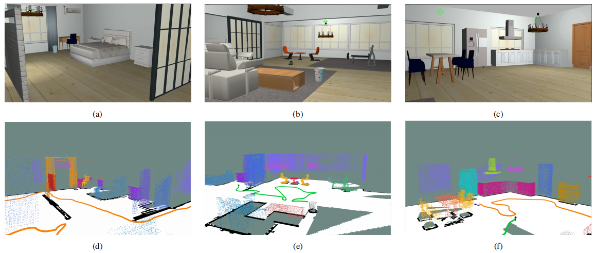
Regional views and corresponding point-cloud clustering results by SGRO
1. Introduction
Simultaneous localization and mapping (SLAM) provides the basis for autonomous navigation and task execution by mobile robots in unknown environments. Classical SLAM jointly estimates robot poses and the environment map, establishing the foundation for persistent perception and self-localization 1,2,3. Multi-robot collaborative SLAM extends environmental coverage and mapping efficiency through information sharing 4,5. Studies on motion planning in dynamic environments, maze navigation, path planning, reinforcement learning, and semantic segmentation have shown the importance of integrating navigation, perception, and decision-making in intelligent robotics 6,7,8,9,10.
Advances in semantic perception and three-dimensional object modeling have enabled SLAM to progress from low-level geometric features toward object-level and semantic representations. Visual SLAM systems provide a foundation for accurate pose estimation 11,12,13,14, and semantic information can be integrated with geometric mapping to support real-time metric-semantic localization and mapping 15. Fusion++, QuadricSLAM, CubeSLAM, and semantic-keypoint object SLAM demonstrate the value of object observations in pose estimation and scene understanding 16,17,18,19. Kimera-Multi, MR-iSAM2, active metric-semantic mapping, and Swarm-SLAM further investigate information sharing, incremental estimation, active perception, and decentralized mapping in multi-robot systems 20,21,22,23.
Asynchronous multi-robot object-level semantic SLAM must address correspondence ambiguity and observation reliability. Repeated layouts can produce similar object arrangements, whereas viewpoint changes and local map updates perturb object positions. CLIPPER organizes candidate correspondences in a consistency graph and selects mutually compatible correspondences through graph optimization 24. Candidate generation can exploit object attributes, and transform acceptance should assess consistency across repeated matching attempts. Object shape also determines orientation observability: similar principal-axis lengths provide weak directional discrimination, so fixed orientation weights can introduce unstable observations into the back end.
We propose SGRO for distributed multi-robot object-level semantic SLAM. SGRO uses semantic–geometric consistency loop-closure detection to reduce association ambiguity and transform fluctuations, together with shape-adaptive robust observation factors to improve the joint estimation of trajectories and object maps.
The main contributions are as follows:
-
1)
A semantic–geometric consistency loop-closure detector jointly uses category, size, and local layout for candidate construction and graph-based association, and combines inlier support, normalized overlap, fault-tolerant confirmation, and quality-based refinement.
-
2)
Robust cuboid and Gaussian ellipsoid observation factors jointly model pose and logarithmic scale errors and adapt rotation weights according to the principal-axis separation ratio.
-
3)
Baseline comparisons and module ablations are conducted in a dual-robot RGB-D indoor simulation using loop-closure, trajectory, and map-level evaluations.
3. Problem Definition
3.1. Relative Pose Transformation and Object-Level Semantic Map
Consider a distributed system with \(n\) robots. Robot \(i\)’s pose at time \(t\) is \(\mathbf{X}_{i}^{t}\in SE(3)\). For \(i,j\in\{1,\ldots,n\}\), \(i\ne j\),
3.2. Loop-Closure Candidate Screening Framework
Cross-robot loop-closure detection matches objects in the maps \(\mathcal{M}_{i}\) and \(\mathcal{M}_{j}\) to estimate the relative transform between robots. Object matching is divided into descriptor pre-screening and pairwise-consistency screening. In the first stage, local triangular structures are constructed in both maps. Semantic–geometric descriptor matching generates candidate pairs \(v_{k_{1}k_{2}}=(o_{k_{1}}^{\,i},o_{k_{2}}^{\,j})\), and all candidate pairs form \(\mathcal{V}_{ij}\subseteq\mathcal{M}_{i}\times\mathcal{M}_{j}\). In the second stage, a candidate-pair consistency graph \(\mathcal{G}_{ij}=(\mathcal{V}_{ij},\mathcal{E}_{ij})\) is constructed. Each node represents a candidate pair, and an edge \(\epsilon_{(k_{1}k_{2})(k_{3}k_{4})}\in\mathcal{E}_{ij}\) represents pairwise consistency between two candidate pairs. Therefore, object matching is formulated as the selection of a consistent candidate-pair subset:
3.3. Object-Observation Model and Back-End Optimization Variables
Let the object observation at time \(t\) be
3.4. Overall Optimization Objective
Overall, the task is to jointly estimate robot poses and the object map under stable cross-robot loop-closure and object-observation constraints. Let the robot-pose and object-state sets be
4. Method
4.1. Method Overview
The framework shown in Fig. 1 consists of a front-end loop-closure constraint generator and back-end joint-optimization module. The front end takes the maps of multiple robots as input and progressively produces stable cross-robot relative-pose constraints through five stages: candidate-pair construction, pairwise-consistency screening, candidate-transform recovery, quality evaluation, and consistency confirmation. The back end jointly optimizes robot poses and object states by incorporating odometry constraints, object-observation constraints, and the cross-robot loop-closure constraints generated by the front end into a unified factor graph, thereby obtaining a consistent estimate of the trajectories and object maps.
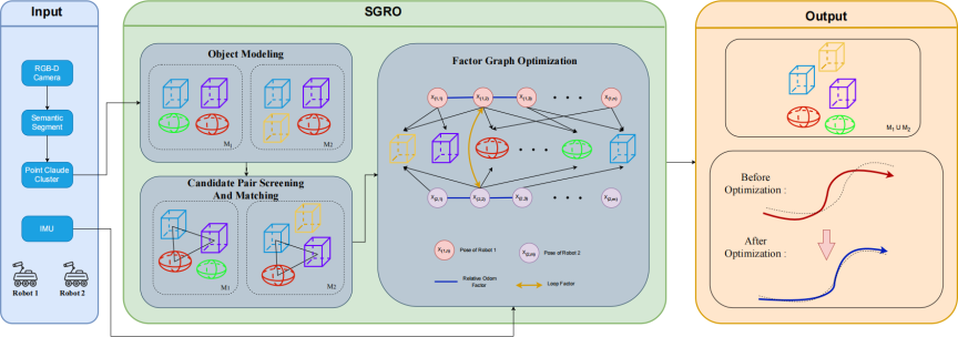
Fig. 1. Overview of the SGRO framework.
4.2. Heterogeneous Geometric Object Observation Factor Modeling
Different geometric objects have different observability and constraint stability. We construct distinct factors for cuboids and Gaussian ellipsoids. The observed pose \(\hat{\boldsymbol{\Gamma}}^{t}\) is mapped to the world frame by the robot pose \(\mathbf{X}^{t}\):
4.2.1. Cuboid Observation Factor
The cuboid observation factor jointly models position, pose, and size. Its residual is
4.2.2. Gaussian Ellipsoid Observation Factor
The observation factor directly models the center, principal-axis orientation, and semi-axis lengths of a Gaussian ellipsoid. Its residual is
4.3. Semantic–Geometric Consistency Loop-Closure Detection
The front end estimates inter-robot transforms from object matching and generates loop-closure constraints after quality evaluation, fault-tolerant confirmation, and refinement.
4.3.1. Initial Candidate-Pair Generation
Semantic–geometric descriptors reduce the search space for candidate matching. For indoor ground robots, object centroids are projected onto the horizontal plane, and Delaunay triangulation 41 is used to construct local triangles from nearby non-collinear objects. For a local triangle \(\pi=(o_{1},o_{2},o_{3})\) in map \(\mathcal{M}\), let \(\bar{\mathbf{p}}_{\pi}\) denote its center and define the vertex descriptor:
4.3.2. Candidate-Pair Consistency Screening
After the initial candidate set \(\mathcal{V}_{ij}\) is generated, a matching graph with candidate pairs as nodes is constructed. For candidate pairs \((k_1,k_2)\) and \((k_3,k_4)\), an edge is established when they do not share an object and preserve the relative distances between the corresponding objects in the two maps. The edge weight is the pairwise consistency score \(s\). For candidate pairs \((k_1,k_2)\) and \((k_3,k_4)\), we define
4.3.3. Candidate Relative-Transformation Recovery
Based on the inlier candidate subset \(\hat{\mathcal{A}}_{ij}\), planar rigid registration estimates the relative rotation and translation between robots \(i\) and \(j\):
4.3.4. Candidate Relative-Pose Quality Measurement
The quality of a candidate relative transform is evaluated using the inlier count and its coverage of the two maps. Let \(n_{ij}=\left|\hat{\mathcal{A}}_{ij}\right|\) denote the number of inlier candidate pairs. The normalized overlap is
4.3.5. Loop-Closure Confirmation and Refinement Update
For transforms from the \(m\)th and \(n\)th matching attempts, let the candidate transforms be \(\hat{\mathbf{T}}_{ij}^{(m)}\) and \(\hat{\mathbf{T}}_{ij}^{(n)}\), with translation components \(\mathbf{t}_{ij}^{(m)}\) and \(\mathbf{t}_{ij}^{(n)}\). Define
4.4. Back-End Factor-Graph Optimization
Unified Optimization Modeling
The cuboid and Gaussian ellipsoid observation factors are substituted into the joint objective function in Section 3. Let \(\mathcal{O}_{\mathrm{cub}}=\{\mathbf{O}_{\mathrm{cub}}\}\) and \(\mathcal{O}_{\mathrm{ell}}=\{\mathbf{O}_{\mathrm{ell}}\}\), which, together with the robot poses, form the back-end optimization variables. The objective function is
5. Experiments
5.1. Experimental Setup
A dual-robot distributed object-level semantic SLAM system was used for the experiments. All configurations used the same Gazebo indoor scene, robot initialization, RGB-D sensors, communication settings, and evaluation protocol. The scene contained tables, chairs, doors, windows, decorations, and household appliances, covering repeated structures, similar object scales, and viewpoint changes. Two ground robots, each carrying the same type of RGB-D camera, were used. Object observations were generated by a YOLOv8-based semantic segmentation model 42. The robots started at different positions, built local maps, and periodically exchanged information for map matching and constraint fusion.
5.2. Baseline, Evaluation Protocol, and Implementation Configuration
SlideSLAM was the baseline method. Both methods used identical scenes, initial poses, sensors, YOLOv8 detections, odometry, and communication. Gazebo model states provided ground truth; trajectory alignment, event filtering, and metric computation followed identical rules. Runtime and communication overhead were recorded with localization and map metrics.
The baseline used SlideGraph’s triangular matching and consistency-graph optimization, and directly accepted the first cross-robot transform. Its back end used the original cuboid model and an ellipsoid observation based on centroid distance and bearing, with linear scale residuals and fixed rotation weights. SGRO used semantic–geometric loop closure with confirmation and refinement, heterogeneous observation factors, adaptive rotation weights, and a robust kernel. The ablation experiments retained either the SGRO loop-closure module or the SGRO observation-factor module.
The baseline used a yaw step of 15\(°\), a minimum inlier count of 1, 30 objects to initialize SlideGraph, a descriptor threshold of 0.2, \(\sigma=0.1\), and \(\epsilon=0.5\). SGRO used a minimum of 6 inlier pairs, minimum of 5 map objects, maximum of 6 repeated-category candidates, 8-neighbor topology, node and edge thresholds of 0.20 and 0.10, topology-quality threshold of 0.30, residual thresholds of 0.80, 1.20, and 0.60, minimum of 5 valid pairs, distance threshold of 1.5 m, residual-score threshold of 1.0, and 10 s computation budget. Candidates required at least 5 inliers, a quality score of 0.30, and three consecutive confirmations. Tentative tolerances were 0.25 m and 5°; refinement required two confirmations and a 30 s refresh interval. The principal-axis transition interval was [1.08, 1.25], the minimum rotation weight was 0.05, and the Huber parameter was 1.5. The consistency graph used the CLIPPER matrix solver with a maximum of 32 nodes. The back end used GTSAM iSAM2 with incremental Cholesky updates and a relinearization threshold of 0.1. The main node ran at 5 Hz, loop closure at 0.2 Hz, and communication waited 5 s.
5.3. Evaluation Metrics
Position Err. [m] denotes the mean translational error of a cross-robot relative-pose constraint; Yaw Err. [deg] denotes the mean yaw error. Standard deviations describe event-to-event variation, and Conf. Rate [%] is the proportion of confirmed events. Absolute trajectory error (ATE) and relative pose error (RPE), reported as position and yaw root mean square error (RMSE), quantify global and local trajectory errors.
5.4. Comparative Experiments
SGRO was compared with SlideSLAM using loop-closure and trajectory metrics. Table 2 shows that SGRO has lower translational and yaw errors for loop-closure estimates, together with lower standard deviations in both directions, indicating more accurate and stable relative-pose estimates. Its confirmation rate is also higher. Table 3 shows lower ATE and RPE errors for both robots. Fig. 2 shows lower medians and more concentrated SGRO distributions.
| Metric | Pair | SlideSLAM | SGRO |
| Pos. Err. [m] | \(1\!\rightarrow\!2\) | 2.1335 | 0.2157 |
| Pos. Err. [m] | \(2\!\rightarrow\!1\) | 2.0145 | 0.2572 |
| Pos. Err. Std [m] | \(1\!\rightarrow\!2\) | 1.5547 | 0.3461 |
| Pos. Err. Std [m] | \(2\!\rightarrow\!1\) | 1.3601 | 0.2466 |
| Yaw Err. [deg] | \(1\!\rightarrow\!2\) | 20.0103 | 1.3421 |
| Yaw Err. [deg] | \(2\!\rightarrow\!1\) | 27.1742 | 1.6971 |
| Yaw Err. Std [deg] | \(1\!\rightarrow\!2\) | 21.1928 | 3.1354 |
| Yaw Err. Std [deg] | \(2\!\rightarrow\!1\) | 25.8449 | 2.5824 |
| Conf. Rate [%] | \(1\!\rightarrow\!2\) | 12.1212 | 56.3633 |
| Conf. Rate [%] | \(2\!\rightarrow\!1\) | 20.0000 | 70.0000 |
| Metric | Robot | SlideSLAM | SGRO |
| ATE Pos. RMSE [m] | Robot1 | 1.7175 | 0.3797 |
| ATE Pos. RMSE [m] | Robot2 | 1.1986 | 0.5751 |
| ATE Yaw RMSE [deg] | Robot1 | 42.6804 | 8.8527 |
| ATE Yaw RMSE [deg] | Robot2 | 21.0971 | 13.3711 |
| RPE Pos. RMSE [m] | Robot1 | 0.2683 | 0.0569 |
| RPE Pos. RMSE [m] | Robot2 | 0.2313 | 0.0796 |
| RPE Yaw RMSE [deg] | Robot1 | 9.7659 | 6.7868 |
| RPE Yaw RMSE [deg] | Robot2 | 6.7548 | 6.5726 |
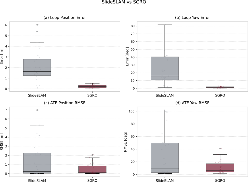
Fig. 2. Error-distribution boxplots for SGRO and the baseline.
5.5. Ablation Experiments
In the ablation experiments, loop_only refers to SGRO loop closure, confirmation, and refinement combined with the baseline back end; graph_only refers to the baseline front end combined with SGRO observation factors and graph optimization. The loop-closure and trajectory results are presented in Tables 4 and 5. Both ablations reduced loop-closure and trajectory errors. Notably, loop_only provided better global position accuracy, whereas graph_only provided better yaw accuracy, demonstrating complementary effects.
Figure 3 compares the error distributions of loop_only and SlideSLAM. Fig. 4 presents the corresponding comparison between graph_only and SlideSLAM. Both configurations showed lower medians and smaller interquartile ranges for loop-closure position and yaw errors and ATE position and yaw RMSE.
| Metric | Pair | SlideSLAM | Loop | Graph |
| Pos. Err. [m] | \(1\!\rightarrow\!2\) | 2.4077 | 0.6245 | 0.7988 |
| Pos. Err. [m] | \(2\!\rightarrow\!1\) | 2.2089 | 0.6951 | 0.5015 |
| Pos. Err. Std [m] | \(1\!\rightarrow\!2\) | 2.0172 | 0.6840 | 0.2626 |
| Pos. Err. Std [m] | \(2\!\rightarrow\!1\) | 1.3601 | 0.5332 | 0.2516 |
| Yaw Err. [deg] | \(1\!\rightarrow\!2\) | 23.1627 | 7.7122 | 6.9247 |
| Yaw Err. [deg] | \(2\!\rightarrow\!1\) | 29.8121 | 8.0652 | 5.7697 |
| Yaw Err. Std [deg] | \(1\!\rightarrow\!2\) | 28.3274 | 7.0897 | 2.6633 |
| Yaw Err. Std [deg] | \(2\!\rightarrow\!1\) | 25.8449 | 6.1092 | 3.2518 |
| Conf. Rate [%] | \(1\!\rightarrow\!2\) | 3.3333 | 42.8330 | – |
| Conf. Rate [%] | \(2\!\rightarrow\!1\) | 11.1111 | 29.6289 | – |
| Metric | Robot | SlideSLAM | Loop | Graph |
| ATE Pos. RMSE [m] | Robot1 | 1.7175 | 0.0284 | 0.0393 |
| ATE Pos. RMSE [m] | Robot2 | 1.1986 | 0.0347 | 0.0392 |
| ATE Yaw RMSE [deg] | Robot1 | 42.6804 | 2.9386 | 2.6933 |
| ATE Yaw RMSE [deg] | Robot2 | 21.0971 | 3.3560 | 2.8814 |
| RPE Pos. RMSE [m] | Robot1 | 0.2683 | 0.0330 | 0.0342 |
| RPE Pos. RMSE [m] | Robot2 | 0.2313 | 0.0390 | 0.0364 |
| RPE Yaw RMSE [deg] | Robot1 | 9.7659 | 3.9312 | 3.6050 |
| RPE Yaw RMSE [deg] | Robot2 | 6.7548 | 4.3136 | 3.5991 |
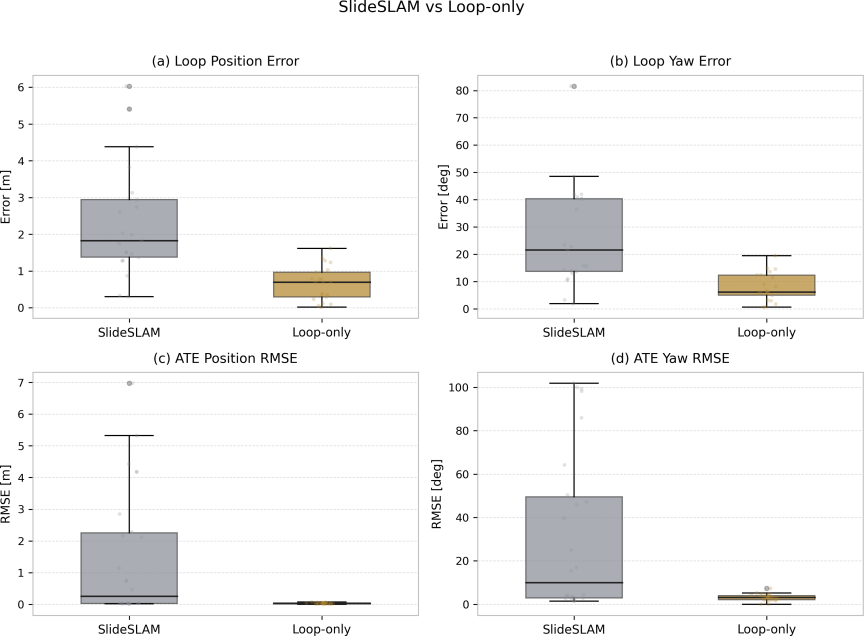
Fig. 3. Error-distribution boxplots for loop_only and the baseline.
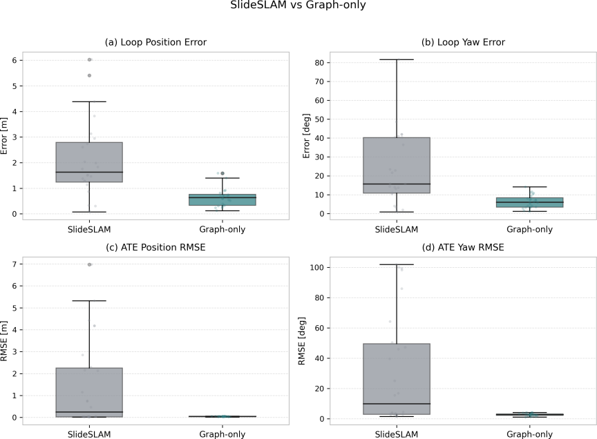
Fig. 4. Error-distribution boxplots for graph_only and the baseline.
5.6. Regional Visualization Results
Figure 5 compares regional scene views with the corresponding point-cloud clustering results. The bedroom, living room, and dining room are shown in Figs. 5(a)–(c), with their clustered maps in Figs. 5(d)–(f), respectively. The clustered objects preserve the main furniture arrangements in these regions, providing a qualitative illustration of the object-level map structure.
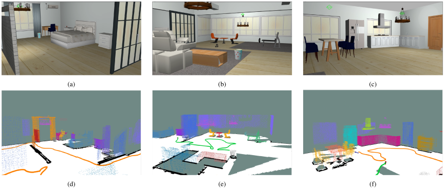
Fig. 5. Regional views and corresponding point-cloud clustering results. (a) Bedroom. (b) Living room. (c) Dining room. (d) Bedroom clustered map. (e) Living-room clustered map. (f) Dining-room clustered map.
5.7. Experimental Analysis
SGRO improves loop-closure accuracy through object-attribute discrimination and cross-attempt consistency constraints. Repeated indoor layouts create similar spatial arrangements, whereas RGB-D observations and viewpoint changes introduce position bias and increase geometric-matching ambiguity. The baseline mainly compares geometric distances during triangular candidate generation. SGRO combines category, size, and local-layout information to distinguish similar layouts, and its consistency confirmation tests candidate stability using subsequent observations. These two designs alleviate candidate ambiguity and transform fluctuation, respectively, and explain the lower loop-closure errors and dispersion observed in this scene. Their effectiveness depends on the distinguishability of shared objects in category, scale, and layout.
Cross-map loop-closure constraints and persistent object observations provide two sources of trajectory improvement. The former corrects relative poses and helps reduce global drift, whereas the latter transfers geometric constraints between adjacent poses and improves local motion estimation. Compared with the baseline ellipsoid observation based on centroid distance and bearing, SGRO uses principal-axis orientation to provide additional pose information and assigns weights according to shape observability: objects with clearly separated principal axes provide stronger directional constraints, whereas nearly symmetric objects receive lower orientation weights. The different RPE yaw improvements of the two robots may be related to the shapes of objects along their trajectories and observation viewpoints.
The runtime and communication overhead are recorded separately for each robot. Factor addition and graph optimization times cover each normally completed observation-processing cycle, including rejected observations, whereas cross-robot loop-closure time covers detection and relative-transform estimation for successful matches. Communication overhead is estimated from the payload transmitted in each communication round, using the mean and maximum values across rounds. The estimated fields include poses and relative odometry (56 B each), cuboid or ellipsoid objects (69 B each), cylindrical objects (37 B), map objects (56 B), object quality (8 B), and inter-robot transforms (58 B). Object counts and trajectory lengths are taken at the end of each run to describe the corresponding map and trajectory scale.
As object counts and trajectory lengths increase, the back end processes more object factors and pose nodes, and candidate construction becomes more expensive; communication overhead also grows with the number of exchanged object observations and pose records. An independent loop-closure thread makes matching and main-node updates asynchronous, while the 5 s communication wait interval equalizes the information-exchange period across configurations.
The experiments validate the accuracy improvement of SGRO in a dual-robot RGB-D indoor simulation, while the applicability of the conclusions is bounded by scene scale, observation conditions, and team size. The experiments do not cover large-scale scenes, outdoor environments, dynamic objects, or larger robot teams. In large scenes, growth in map and candidate-matching scale increases the computational burden, and a lower map overlap can reduce the shared objects for loop-closure confirmation. Outdoor illumination changes, long-range observations, and differences in object distributions impose stronger requirements on the stability of semantic detection and geometric estimation. Dynamic objects change spatial relations and affect consistency judgments based on static object layouts. More robots also create additional cross-robot matching tasks and communication and map-synchronization overhead. Simulation provides limited coverage of real sensor errors and communication fluctuations. Real-robot experiments and scale-expansion evaluations are therefore required to assess robustness and scalability under these conditions, with localization accuracy, loop-closure reliability, runtime, and communication volume evaluated jointly.
6. Conclusion
This paper presents SGRO for distributed multi-robot object-level semantic SLAM. Semantic–geometric descriptors and candidate-pair consistency optimization form the loop-closure detector, whereas fault-tolerant confirmation and refinement improve the stability of cross-robot constraints. Shape-adaptive robust observation factors use object pose and scale information for joint trajectory and map optimization. In dual-robot RGB-D indoor simulation, SGRO reduced loop-closure and trajectory errors, and ablations further showed the complementary effects of the two modules on position and orientation estimation.
Future work will evaluate the method using real robots and larger teams, investigate joint optimization of map uncertainty and trajectory planning for active mapping, and explore high-level relational reasoning based on object-semantic knowledge graphs.
Acknowledgments
This work is supported by the National Key Research and Development Program of China (No.2022YFB4201603), the “Pioneer” and “Leading Goose” R&D Program of Zhejiang (No.2024SJCZX0005), the National Natural Science Foundation of China (No.61873033), the State Key Laboratory of Industrial Control Technology, China (ICT2026C03, ICT2025C02) and the Science and Technology Project Foundation of Fujian Province (No.2024H0012, No.JAT251264).
- [1] M. W. M. G. Dissanayake, P. Newman, S. Clark et al., “A solution to the simultaneous localization and map building (SLAM) problem,” IEEE Trans. Robotics Autom., Vol.17, No.3, pp. 229-241, 2001. https://doi.org/10.1109/70.938381
- [2] T. Bailey and H. Durrant-Whyte, “Simultaneous localization and mapping (SLAM): Part II,” IEEE Robotics Autom. Mag., Vol.13, No.3, pp. 108-117, 2006. https://doi.org/10.1109/MRA.2006.1678144
- [3] C. Cadena, L. Carlone, H. Carrillo et al., “Past, present, and future of simultaneous localization and mapping: Toward the robust-perception age,” IEEE Trans. Robotics, Vol.32, No.6, pp. 1309-1332, 2016. https://doi.org/10.1109/TRO.2016.2624754
- [4] S. B. Williams, G. Dissanayake, and H. Durrant-Whyte, “Towards multi-vehicle simultaneous localisation and mapping,” Proc. 2002 IEEE Int. Conf. on Robotics and Automation, pp. 2743-2748, 2002. https://doi.org/10.1109/ROBOT.2002.1013647
- [5] P.-Y. Lajoie, B. Ramtoula, F. Wu et al., “Towards collaborative simultaneous localization and mapping: A survey of the current research landscape,” Field Robotics, Vol.2, pp. 971-1000, 2022. https://doi.org/10.55417/fr.2022032
- [6] S. Hoshino and K. Uchida, “Interactive motion planning for mobile robot navigation in dynamic environments,” J. Adv. Comput. Intell. Intell. Informatics, Vol.21, pp. 667-674, 2017. https://doi.org/10.20965/jaciii.2017.p0667
- [7] X. Zhang, Y. Liu, L. Wang et al., “A curiosity-based autonomous navigation algorithm for maze robot,” J. Adv. Comput. Intell. Intell. Informatics, Vol.26, No.6, pp. 893-904, 2022. https://doi.org/10.20965/jaciii.2022.p0893
- [8] S. X. Yang and M. Meng, “An efficient neural network model for path planning of car-like robots in dynamic environment,” J. Adv. Comput. Intell. Intell. Informatics, Vol.4, No.3, pp. 220-229, 2000. https://doi.org/10.20965/jaciii.2000.p0220
- [9] J. Wang, K. Hirota, X. Wu, Y. Dai, and Z. Jia, “Hybrid bidirectional rapidly exploring random tree path planning algorithm with reinforcement learning,” J. Adv. Comput. Intell. Intell. Inform., Vol.25, No.1, pp. 121-129, 2021. https://doi.org/10.20965/jaciii.2021.p0121
- [10] R. P. Rangkuti, V. Dewanto, Aprinaldi et al., “Utilizing google images for training classifiers in CRF-based semantic segmentation,” J. Adv. Comput. Intell. Intell. Informatics, Vol.20, pp. 455-461, 2016. https://doi.org/10.20965/jaciii.2016.p0455
- [11] R. Mur-Artal, J. M. M. Montiel, and J. D. Tardós, “ORB-SLAM: A versatile and accurate monocular SLAM system,” IEEE Trans. Robotics, Vol.31, No.5, pp. 1147-1163, 2015. https://doi.org/10.1109/TRO.2015.2463671
- [12] R. Mur-Artal and J. D. Tardós, “ORB-SLAM2: An open-source system for monocular, stereo, and RGB-D cameras,” IEEE Trans. Robotics, Vol.33, No.5, pp. 1255-1262, 2017. https://doi.org/10.1109/TRO.2017.2705103
- [13] C. Campos, R. Elvira, J. J. Gómez Rodríguez et al., “ORB-SLAM3: An accurate open-source library for visual, visual-inertial, and multi-map SLAM,” IEEE Trans. Robotics, Vol.37, No.6, pp. 1874-1890, 2021. https://doi.org/10.1109/TRO.2021.3075644
- [14] T. Qin, P. Li, and S. Shen, “VINS-Mono: A robust and versatile monocular visual-inertial state estimator,” IEEE Trans. Robotics, Vol.34, No.4, pp. 1004-1020, 2018. https://doi.org/10.1109/TRO.2018.2853729
- [15] A. Rosinol, M. Abate, Y. Chang et al., “Kimera: An open-source library for real-time metric-semantic localization and mapping,” 2020 IEEE Int. Conf. on Robotics and Automation (ICRA), pp. 1689-1696, 2020. https://doi.org/10.1109/ICRA40945.2020.9196885
- [16] J. McCormac, R. Clark, M. Bloesch et al., “Fusion++: Volumetric object-level SLAM,” 2018 Int. Conf. on 3D Vision (3DV), pp. 32-41, 2018. https://doi.org/10.1109/3DV.2018.00015
- [17] L. Nicholson, M. Milford, and N. Sünderhauf, “QuadricSLAM: Dual quadrics from object detections as landmarks in object-oriented SLAM,” IEEE Robotics Autom. Lett., Vol.4, No.1, pp. 1-8, 2019. https://doi.org/10.1109/LRA.2018.2866205
- [18] S. Yang and S. Scherer, “CubeSLAM: Monocular 3-D object SLAM,” IEEE Trans. Robotics, Vol.35, No.4, pp. 925-938, 2019. https://doi.org/10.1109/TRO.2019.2909168
- [19] S. L. Bowman, K. Daniilidis, and G. J. Pappas, “Robust object-level semantic visual SLAM using semantic keypoints,” Field Robotics, Vol.2, pp. 513-524, 2022. https://doi.org/10.55417/fr.2022018
- [20] Y. Tian, Y. Chang, F. Herrera Arias et al., “Kimera-Multi: Robust, distributed, dense metric-semantic SLAM for multi-robot systems,” IEEE Trans. Robotics, Vol.38, No.4, pp. 2022-2038, 2022. https://doi.org/10.1109/TRO.2021.3137751
- [21] Y. Zhang, M. Hsiao, J. Dong et al., “MR-iSAM2: Incremental smoothing and mapping with multi-root Bayes tree for multi-robot SLAM,” 2021 IEEE/RSJ Int. Conf. on Intelligent Robots and Systems (IROS), pp. 8671-8678, 2021. https://doi.org/10.1109/IROS51168.2021.9636687
- [22] X. Liu, A. Prabhu, F. Cladera et al., “Active metric-semantic mapping by multiple aerial robots,” 2023 IEEE Int. Conf. on Robotics and Automation (ICRA), pp. 3282-3288, 2023. https://doi.org/10.1109/ICRA48891.2023.10161564
- [23] P.-Y. Lajoie and G. Beltrame, “Swarm-SLAM: Sparse decentralized collaborative simultaneous localization and mapping framework for multi-robot systems,” arXiv:2301.06230, 2023. https://doi.org/10.48550/arXiv.2301.06230
- [24] P. C. Lusk, K. Fathian, and J. P. How, “CLIPPER: A graph-theoretic framework for robust data association,” arXiv:2011.10202, 2020. https://doi.org/10.48550/arXiv.2011.10202
- [25] M. Kaess, A. Ranganathan, and F. Dellaert, “iSAM: Incremental smoothing and mapping,” IEEE Trans. Robotics, Vol.24, No.6, pp. 1365-1378, 2008. https://doi.org/10.1109/TRO.2008.2006706
- [26] M. Kaess, H. Johannsson, R. Roberts et al., “iSAM2: Incremental smoothing and mapping using the Bayes tree,” Int. J. Robotics Research, Vol.31, No.2, pp. 216-235, 2012. https://doi.org/10.1177/0278364911430419
- [27] F. Dellaert and M. Kaess, “Factor graphs for robot perception,” Found. Trends Robotics, Vol.6, Nos.1-2, pp. 1-139, 2017. https://doi.org/10.1561/2300000043
- [28] L. Schmid, J. Delmerico, J. L. Schönberger et al., “Panoptic multi-TSDFs: A flexible representation for online multi-resolution volumetric mapping and long-term dynamic scene consistency,” 2022 Int. Conf. on Robotics and Automation (ICRA), pp. 8018-8024, 2022. https://doi.org/10.1109/ICRA46639.2022.9811877
- [29] K. Sirohi, D. Büscher, and W. Burgard, “uPLAM: Robust panoptic localization and mapping leveraging perception uncertainties,” IEEE Robotics Autom. Lett., Vol.9, No.8, pp. 7174-7181, 2024. https://doi.org/10.1109/LRA.2024.3419648
- [30] A. Adkins, T. Chen, and J. Biswas, “ObVi-SLAM: Long-term object-visual SLAM,” IEEE Robotics Autom. Lett., Vol.9, No.3, pp. 2909-2916, 2024. https://doi.org/10.1109/LRA.2024.3363534
- [31] Y. Wu, Y. Zhang, D. Zhu et al., “An object SLAM framework for association, mapping, and high-level tasks,” IEEE Trans. on Robotics, Vol.39, No.4, pp. 2912-2932, 2023. https://doi.org/10.1109/TRO.2023.3273180
- [32] G. Grisetti, R. Kümmerle, C. Stachniss et al., “A tutorial on graph-based SLAM,” IEEE Intell. Transportation Systems Mag., Vol.2, No.4, pp. 31-43, 2010. https://doi.org/10.1109/MITS.2010.939925
- [33] M. Cummins and P. Newman, “FAB-MAP: Probabilistic localization and mapping in the space of appearance,” Int. J. Robotics Research, Vol.27, No.6, pp. 647-665, 2008. https://doi.org/10.1177/0278364908090961
- [34] D. Gálvez-López and J. D. Tardós, “Bags of binary words for fast place recognition in image sequences,” IEEE Trans. Robotics, Vol.28, No.5, pp. 1188-1197, 2012. https://doi.org/10.1109/TRO.2012.2197158
- [35] R. Arandjelović, P. Gronat, A. Torii et al., “NetVLAD: CNN architecture for weakly supervised place recognition,” 2016 IEEE Conf. on Computer Vision and Pattern Recognition (CVPR), pp. 5297-5307, 2016. https://doi.org/10.1109/CVPR.2016.572
- [36] G. Kim and A. Kim, “Scan context: Egocentric spatial descriptor for place recognition within 3D point cloud map,” 2018 IEEE/RSJ Int. Conf. on Intelligent Robots and Systems (IROS), pp. 4802-4809, 2018. https://doi.org/10.1109/IROS.2018.8593953
- [37] R. Dubé, A. Cramariuc, D. Dugas et al., “SegMap: Segment-based mapping and localization using data-driven descriptors,” Int. J. Robotics Research, Vol.39, Nos.2-3, pp. 339-355, 2020. https://doi.org/10.1177/0278364919863090
- [38] X. Liu, J. Lei, A. Prabhu et al., “SlideSLAM: Sparse, lightweight, decentralized metric-semantic SLAM for multirobot navigation,” IEEE Trans. Robotics, Vol.41, pp. 6529-6548, 2025. https://doi.org/10.1109/TRO.2025.3629786
- [39] R. Zhang, H. M. Bong, and G. Beltrame, “Active semantic mapping and pose graph spectral analysis for robot exploration,” 2024 IEEE/RSJ Int. Conf. on Intelligent Robots and Systems (IROS), pp. 13787-13794, 2024. https://doi.org/10.1109/IROS58592.2024.10802821
- [40] A. Asgharivaskasi, F. Girke, and N. Atanasov, “Riemannian optimization for active mapping with robot teams,” IEEE Trans. on Robotics, Vol.41, pp. 1077-1097, 2025. https://doi.org/10.1109/TRO.2025.3526295
- [41] R. A. Dwyer, “A faster divide-and-conquer algorithm for constructing delaunay triangulations,” Algorithmica, Vol.2, No.1-4, pp. 137-151, 1987. https://doi.org/10.1007/BF01840356
- [42] M. Yaseen, “What is YOLOv8: An in-depth exploration of the internal features of the next-generation object detector,” arXiv:2408.15857, 2024. https://doi.org/10.48550/arXiv.2408.15857
This article is published under a Creative Commons Attribution-NoDerivatives 4.0 Internationa License.