
Research Paper:
CxLSTM: Deploying xLSTM-Based Custom Keyword Spotting to Edge Devices
Haitao Cao
 , Tianyou Xiao, Chao Chang
, Luyao Teng
, Xi Liu†
, and Dan Deng
School of Information Engineering, Guangzhou Polytechnic University
No.1342 Shiliang Road, Shawan Street, Panyu District, Guangzhou, Guangdong 511483, China
†Corresponding author

Keyword spotting (KWS) serves as the critical entry point for voice interaction in intelligent systems. Traditional KWS systems rely on predefined keywords with limited customization, whereas existing custom keyword spotting (CKWS) approaches incur heavy computational overhead, limiting their deployment on resource-limited edge devices. To address these challenges, we present CxLSTM, an optimized extended LSTM module with only 57.6K parameters, 318.6 KB static memory, 593.1 KB peak memory, and 3.54 MACs per inference. Based on CxLSTM, we propose an on-device CKWS method and perform extensive experiments. In offline evaluation, the proposed method obtains an equal error rate (EER) of 0.27 and an area under the ROC curve (AUC) of 0.78 on the public Google Speech Commands V2 dataset. Superior performance is further validated on a private Mandarin dataset, yielding an EER of 0.06 and an AUC of 0.98. Furthermore, in real-world tests for Mandarin CKWS across three scenarios, the proposed method achieves a recognition accuracy above 95% on Android devices, with a false alarm rate below 0.75/24 h and an average latency of 2.1 ms. When deployed on STM32 microcontrollers, it maintains an accuracy of over 92.3%, with moderately increased false alarms (15.8/24 h) and latency (264.7 ms). Despite performance degradation on low-power microcontrollers due to limited hardware resources, the proposed CKWS method still enables efficient voice interaction on edge devices.
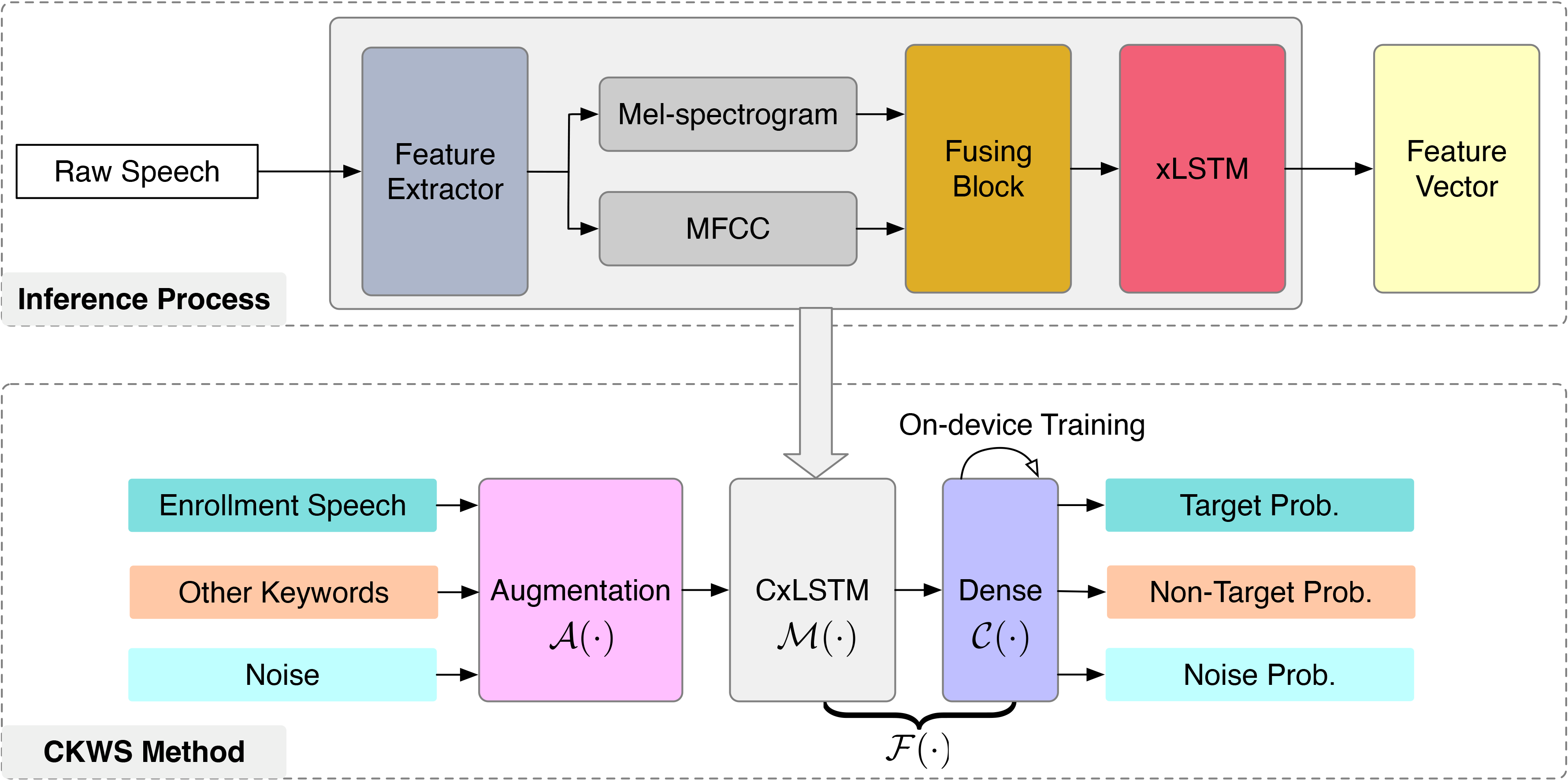
Custom keyword spotting with CxLSTM
1. Introduction
With the rapid advancement of artificial intelligence technologies, human-computer interaction (HCI) has found increasingly intelligent applications 1. Compared with visual interfaces or traditional touch-based interaction modes, voice-based interactions provide a more natural and convenient way for users to communicate with edge devices. Voice interaction enhances the user experience and operational efficiency by enabling devices to accurately understand and respond to spoken commands. As a result, voice interaction has become an indispensable component of modern intelligent systems 2,3.
The typical workflow of a voice-interaction system comprises three principal stages: speech recognition, semantic understanding, and speech synthesis. Speech recognition serves as the foundational step, wherein the system transcribes spoken input into a textual form to enable subsequent processing 4,5. However, in real-world applications, continuous audio monitoring is both power-intensive and prone to false alarms, particularly in noisy surroundings or multiperson conversation scenarios. Consequently, most voice interaction systems operate in a low-power mode and are activated only upon the detection of a predefined wake-up word. This mechanism, commonly referred to as wake-up word detection or keyword spotting (KWS), plays a critical role in HCI systems.
In general, KWS applications require low response latency and power consumption on edge devices, which typically feature a low-performance CPU or MCU without a GPU and limited hardware resources 6,7. Although deep neural networks (DNNs) are preferable for achieving favorable KWS performance in terms of a high wake-up rate and low false alarms, their massive number of parameters and high computational complexity conflict with KWS applications. Therefore, a tradeoff between KWS performance and hardware resources is essential for practical deployment.
In addition, most commercial voice assistants rely on fixed, factory-defined keywords such as “Xiaoai Tongxue” or “Hey Siri.” Although these predefined keywords exhibit robust performance in controlled environments, their ubiquity and phonetic similarity to real-world samples can easily result in unintended activation 8,9. The lack of customization capability also limits personalization, potentially degrading user experience 10. Therefore, there is a growing demand for customizable KWS systems that allow users to define their own wake-up words 10,11.
Custom keyword spotting (CKWS) refers to the capability of a KWS system to recognize user-defined keywords rather than restricting it to a fixed vocabulary. Deploying CKWS on edge devices is often preferred because of the advantages of preserving user privacy, reducing response latency, and improving user experience. Nevertheless, many existing CKWS approaches are computationally intensive 12,13, rendering them unsuitable for resource-limited edge devices. An effective on-device CKWS solution must carefully balance model performance, memory footprint, and computational efficiency.
To this end, this study presents a lightweight and efficient CKWS solution for edge devices. Our key contributions are threefold.
-
1.
We propose CxLSTM, a portable C implementation of the extended long short-term memory (xLSTM) backbone, which enables efficient CKWS on edge devices.
-
2.
We designed a modular online training CKWS pipeline comprising three components: a fixed data-augmentation module (\(\mathcal{A}\)), a quantized CxLSTM encoder (\(\mathcal{M}\)), and a lightweight, trainable classification head (\(\mathcal{C}\)). Only \(\mathcal{C}\) was fine-tuned during on-device CKWS, ensuring minimal computational overhead.
-
3.
We conducted comprehensive experiments, including offline evaluation on a PC and extensive real-world testing on Android and STM32 devices, to demonstrate the effectiveness of the proposed CKWS method.
The remainder of this paper is organized as follows. Section 2 reviews the backbones and customization schemes for KWS. Section 3 details the crucial CxLSTM module and presents a quantitative analysis of its resource overhead. Section 4 proposes a novel CKWS method based on CxLSTM. The offline evaluation and real-world testing of the proposed method are presented in Sections 5 and 6, respectively. Section 7 provides an in-depth discussion, and Section 8 concludes the paper.
2. Related Work
2.1. Backbones for KWS
KWS aims to detect predefined keywords from continuous speech streams and has become a fundamental component of voice-interactive systems. Early deep learning-based KWS studies primarily relied on conventional DNN architectures. The study in 14 first demonstrated the effectiveness of compact convolutional neural network architectures for small-footprint KWS, achieving superior performance. Subsequently, long short-term memory (LSTM) 15 and convolutional recurrent neural networks 16 were introduced to capture temporal dependencies in speech signals, leading to further improvements in recognition accuracy. Despite their effectiveness, these generic architectures are not specifically optimized for KWS scenarios and often exhibit limitations in terms of parameter efficiency and computational cost when deployed on resource-limited devices.
To address these challenges, various lightweight architectures specifically designed for KWS have been proposed. MatchboxNet 17 employs depthwise separable convolutions and residual connections to significantly reduce the model complexity while maintaining competitive performance. BC-ResNet 18 introduced broadcast residual learning to enhance feature representation efficiency and achieved state-of-the-art accuracy under strict computational budgets. In addition, temporal modeling-oriented architectures, such as TENet 19 and token-mixing-based models derived from MLP-Mixer 20, have demonstrated promising results by improving the extraction of discriminative temporal information from acoustic features. These studies indicate that task-specific architectural design is crucial for achieving an optimal tradeoff between recognition performance and computational efficiency in practical KWS applications.
The success of transformer architectures in natural language processing 21 and speech recognition 4 motivated their application to KWS tasks. Representative studies, including KWT 22 and LeTR 23, leverage self-attention mechanisms 22 to model long-range contextual dependencies and achieve competitive performance. Nevertheless, the computational complexity of the self-attention operation scales quadratically with the input sequence length, that is, \(\mathcal{O}(N^2)\), where \(N\) denotes the sequence length. Consequently, transformer-based models generally require more computational and memory resources than conventional lightweight architectures, which limits their applicability to latency-sensitive and resource-limited edge devices. Although several efficient transformer variants have been proposed 24,25, reducing the computational overhead while preserving the strong sequence-modeling capability remains an active research topic in KWS.
Recently, xLSTM has emerged as a new recurrent sequence modeling framework that extends the conventional LSTM architecture 26. Unlike standard LSTM, xLSTM introduces exponential gating mechanisms and enhanced memory structures, namely, scalar-memory LSTM (sLSTM) and matrix-memory LSTM (mLSTM), to improve memory utilization, long-range dependency modeling, and training stability. Furthermore, the matrix-based memory-update mechanism enables efficient parallel training while retaining the recurrent inference characteristics of LSTM. Recent studies demonstrated the effectiveness of xLSTM in audio representation 27 and computer vision 28, achieving performances comparable to or exceeding those of transformer-based architectures. Importantly, the recurrent computation of xLSTM exhibits an approximately linear complexity with respect to the sequence length \(\mathcal{O}(N)\), which is substantially lower than the quadratic complexity of transformer self-attention. This characteristic makes xLSTM particularly attractive for edge-oriented speech applications that require low latency and limited computational resources.
2.2. CKWS Methods
KWS systems typically employ DNNs trained on large-scale datasets that contain a closed set of predefined keywords. Adapting such systems to new keywords usually requires the collection of numerous target samples and the retraining of the entire model. This is referred to as closed-set training 29, which is time-consuming and impractical for on-device customization.
By contrast, open-set training seeks to learn generalization representations, enabling flexible keyword customization without exhaustive retraining. One prominent paradigm is query-by-string (QbS) 30, where users specify new keywords through text input. However, in real-world scenarios, this method requires users to have a standard pronunciation; otherwise, the wake-up rate is low.
Another widely used open-set approach is query-by-example (QbE), which requires a minimal amount of user-provided data 31 and is well-suited for edge deployment 12,6. QbE operates in two phases: (1) enrollment, where template embeddings are extracted from a small number of target keyword samples, and (2) detection, where the incoming speech is compared with these templates using a similarity metric (e.g., dynamic time warping or cosine distance). If the computed similarity score exceeds a predefined threshold, the incoming speech is classified as containing the target keyword. This two-stage framework supports data-efficient CKWS 8,20,32.
Some researchers frame CKWS as a specialized task in automatic speech recognition that leverages large vocabulary continuous speech recognition (LVCSR) techniques 12,13,32. These methods train large-scale models on extensive vocabulary datasets and employ a decoder to search for target keywords, thereby eliminating the need for retraining. However, the high model complexity and substantial parameter count impose prohibitive computational and memory demands 33,34,35. Consequently, LVCSR-based CKWS is frequently deployed in cloud-centric architectures, raising concerns regarding user privacy 36,37 and network-induced latency 38,39. Moreover, recent studies indicate that LVCSR-based systems generalize poorly under real-world acoustic variability, speaker diversity, and out-of-vocabulary conditions 8,20.
In addition to LVCSR, Ref. 40 combined few-shot learning and transfer learning to achieve a CKWS across diverse linguistic contexts. In addition, multimodal learning has been explored for CKWS in 41,42, but it requires the collection and alignment of additional textual datasets, introducing preprocessing burdens and complicating deployment in resource-limited settings.
Motivated by the strong sequence modeling capability and favorable computational efficiency of xLSTM, our previous study 43 investigated the application of xLSTM to KWS and proposed a lightweight xLSTM-based architecture that achieved an improved balance between recognition accuracy and deployment efficiency. This study builds upon our previous work by deploying the xLSTM-based architecture to edge devices and comprehensively evaluating the performance of the proposed on-device CKWS in real-world environments.
We adopted the methods in 6 and 40 as primary comparison baselines. The method in 6 is a CKWS method deployable on edge devices and is highly aligned with the research objective of this study. The method in 40 presented a CKWS method dedicated to multilingual scenarios, which provides a significant reference for our proposed method for implementing multilingual CKWS.
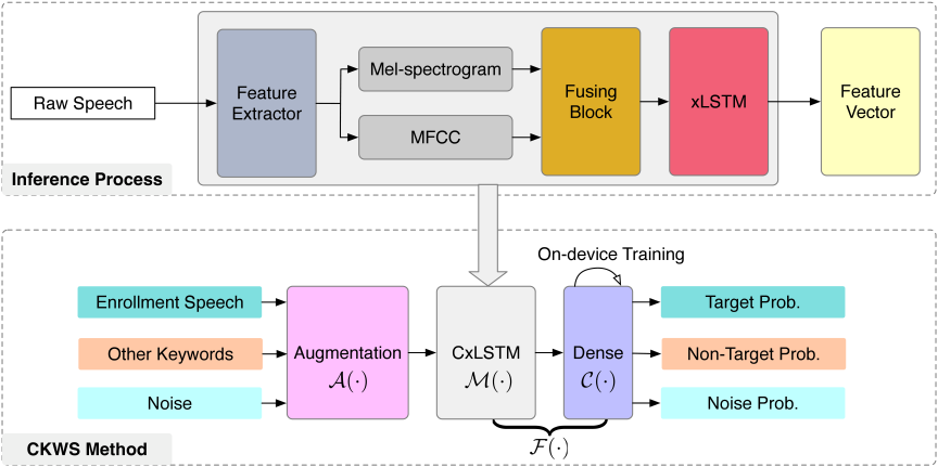
Fig. 1. Framework overview. Top: inference process of the previous work 43. Bottom: on-device CKWS workflow based on CxLSTM.
3. CxLSTM Module
3.1. Overview
As illustrated in the top panel of Fig. 1, in our previous work 43, the xLSTM-based backbone processed raw speech (16 kHz sampling rate) by first extracting the mel-spectrogram and mel-frequency cepstral coefficient (MFCC) features. These features are then fused and fed into a multilayer xLSTM block comprising one mLSTM and one sLSTM layer to produce a high-level embedding representation. In this study, we implemented an xLSTM-based backbone in pure C, that is, CxLSTM, and proposed an on-device CKWS method, as depicted in the bottom panel of Fig. 1.
Before describing the proposed on-device CKWS method, we conducted resource analyses for CxLSTM on a PC. First, in Section 3.2, we perform dynamic quantization on CxLSTM and compare the different quantization methods and precisions. Subsequently, we analyze the memory usage for a specific quantized CxLSTM in Section 3.3. Finally, in Section 3.4, the MACs are calculated to estimate the computational complexity of CxLSTM. These analyses of memory and MACs have also been performed in other related studies for comparison.
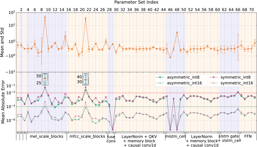
Fig. 2. Top: distribution of original float32 parameters. Bottom: MAE under various quantization schemes. Red and green horizontal lines denote error levels of \(10^{-2}\) and \(10^{-4}\), respectively. Two violin subfigures show the mean (orange lines) and standard deviation (gray lines) values of the parameter sets indexed by 9 and 21, respectively.
3.2. Dynamic Quantization
The acoustic frontend (Hanning window, Mel filter banks, DCT tables) and model parameters of the xLSTM constitute a total of 71 parameter sets. In this study, we use \(\mathbf{u}^i=\{u_1^i,u_2^i,\ldots,u_{M_i}^i\}\) to represent the \(i\)-th parameter set with \(M_i\) parameters, and \(i=1,\ldots,71\). These parameters are all float type with 32 bits (float32), and their distribution is illustrated in the top panel of Fig. 2.
In quantization, the float32 parameters can be quantized to be 8-bit and 16-bit integers for less resource consumption, which we refer to as int8 and int16 quantization precision, respectively. In this study, we compared two quantization methods: i.e., symmetric and asymmetric quantization. Symmetric quantization assumes zero-centered distributions and omits the zero points. Mathematically, for the \(i\)-th parameter set \(\mathbf{u}^i\), the quantization and dequantization processes can be written as:
Note that the \(\mathrm{round}\) function is the standard rounding function and defined as \(\mathrm{round}(x) = \lfloor x + 0.5 \rfloor\). The \(\mathrm{clip}\) function that restricts a value \(x\) to a given range \([m,n]\) is defined as
Accordingly, asymmetric quantization handles skewed distributions more effectively by introducing zero points. The asymmetric quantization and its dequantization process can be written as
To compare the different quantization methods (symmetric and asymmetric) and quantization precisions (int8 and int16), the mean absolute error (MAE) between the original float32 type parameter set \(\mathbf{u}^i\) and the reconstructed set \(\mathbf{r}^i\) was computed as:
All the MAEs under various quantization schemes are illustrated in the bottom panel of Fig. 2. We found that the MAEs of the two parameter sets indexed by 9 and 21, that is, \(\varepsilon_9\) and \(\varepsilon_{21}\), exceeded error levels of \(10^{-2}\) or \(10^{-4}\), respectively. By observing the violin subfigures, we found that the distributions of these two parameter sets are skewed over a large dynamic range, which reduces quantization precision. These parameters belong to the “running_var” of the BatchNorm layers. Large “running_var” values indicate that the training data have strong sample diversity, which enhances the generalization of models. Furthermore, asymmetric quantization appears to be slightly better than symmetric quantization. Considering the 50% storage saving of int8, we select asymmetric int8 quantized CxLSTM for subsequent analysis and deployment.
Note that dynamic quantization only reduces storage overhead (e.g., ROM and Flash on edge devices) but cannot lower runtime memory consumption. This is because the quantized parameters must be de-quantized into floating-point values for computation during inference. Therefore, we report the number of model parameters listed in Table 1 (the “Params.” column), which directly indicates the differences in model size.
3.3. Memory Analysis
In this section, we analyze the memory usage of asymmetric int8 quantized CxLSTM. Static memory is allocated by the compiler at the compilation stage, and the size is fixed. We used the size command to check the static memory of the Linux platform. It was found that CxLSTM required 326,238 bytes of static memory, approximately 318.6 KB. The details are as follows:
-
・
text: shows the machine instructions for storing programs, occupying 88,174 bytes (86.11 KB). -
・
data: shows the global and static variables assigned during compilation, occupying 2,660 bytes (2.60 KB). -
・
bss: shows the global and static variables that are not assigned at compile time, occupying 235,404 bytes (229.89 KB).
Dynamic memory is mainly allocated by malloc or calloc functions at runtime. We used the valgrind command as the core tool and found that the peak memory usage was 607,352 bytes (approximately 593.12 KB), including 607,296 bytes for our task and 56 bytes for memory management. This implies that the memory utilization rate is very high, with only 0.009% management overhead. We list the distribution of peak memory usage as follows:
-
・
55.54% (337,280 bytes) for the inference process of xLSTM;
-
・
26.35% (160,000 bytes) for loading speech data;
-
・
18.11% (110,016 bytes) for feature extraction, of which 1.78% (10,816 bytes) was used for FFT computation.
We compared the memory consumption of our CxLSTM with that of the CRNN model in 6 and the EfficientNet model in 40, as shown in Table 1. The results show that both CxLSTM and CRNN significantly outperform EfficientNet; however, CxLSTM consumes more memory than CRNN, especially in terms of peak memory usage. This is mainly attributed to the contextual gating mechanism and dynamic state buffer structure adopted in xLSTM 26, which introduce extra memory overhead for intermediate variables while preserving a strong temporal modeling capability. In contrast, the CRNN adopts fixed-length sliding windows and weight-sharing convolutions to achieve more compact memory allocation at the cost of degraded long-range dependency modeling performance. In our future work, we plan to further reduce the memory footprint of CxLSTM via lightweight contextual gating designs and state-buffer compression strategies.
3.4. Multiply-Accumulate Operations (MACs)
MACs quantify the total multiply-accumulate computations consumed during model inference and act as core metrics for assessing the model computational complexity. In this work, we employ the torchinfo library built on the PyTorch framework to analyze model architectures, resolve layer-wise MACs distributions, and aggregate the overall MAC overhead, with full results summarized in Table 1. MACs profiling was conducted on the original floating-point model prior to quantization. Because quantization compresses the model storage without altering the total number of MACs, the MAC values summarized in Table 1 are equally representative of the computational complexity of their quantized counterparts.
4. Keyword Customization on Device
Based on CxLSTM, the proposed CKWS method leverages the online supervised fine-tuning of a lightweight neural architecture, formulated as a three-class classification problem, as shown in the bottom panel of Fig. 1. The enrollment process for keyword customization is described in Section 4.1, and the inference process for testing is described in Section 4.2.
4.1. Enrollment Process
4.1.1. Data Preparation
The user recorded three samples of the new keywords. These samples constitute the positive class (target) for customization. To form a balanced three-class classification task, two auxiliary classes are introduced: (i) prerecorded canonical keywords (e.g., xiao3 ai4 tong2 xue2 from Xiaomi), and (ii) noise segments collected in a real-world environment. Let \(\mathfrak{D}_{\text{raw}} = \{ \mathbf{x}_i, y_i \}_{i=1}^{N_0}\), where \(\mathbf{x}_i\in\mathbb{R}^{L}\) is one sample, and \(L\) is its length. \(N_0\) is the number of source data points, and \(y_i \in \{0,1,2\}\) denotes the labels for the target, canonical, and noise classes, respectively.
4.1.2. Augmentation and Feature Extraction
To enhance robustness and mitigate overfitting given the limited source data \(\mathfrak{D}_{\text{raw}}\), we apply a composite augmentation strategy modeled as a stochastic transformation \(\mathcal{A}(\cdot)\). Specifically, \(\mathcal{A}\) integrates augmentation in both the time domain and time-frequency domains with SpecAugment 44 and Cutout 45.
The augmented dataset is denoted as \(\mathfrak{D}_{\text{aug}} = \{ \mathcal{A}(\mathbf{x}_i), y_i \}_{i=1}^{N}\), where \(N\gg{N_0}\). Subsequently, CxLSTM acts as an encoder \(\mathcal{M}(\cdot)\), yielding a temporal sequence of hidden states:
4.1.3. Classifier Training
The classification head \(\mathcal{C}(\cdot)\) consists of two dense layers and forms a shallow feedforward network. The parameters \(\boldsymbol{\theta}_{\mathcal{C}}\) were updated via mini-batch stochastic gradient descent. Specifically, the augmented dataset \(\mathfrak{D}_{\text{aug}}\) containing \(N\) samples was partitioned into \(K=\left \lceil N/B \right \rceil\) disjoint minibatches, where \(B\) denotes a predefined batch size. The first \(K−1\) batches each contain exactly \(B\) samples, while the \(K\)-th (final) batch consists of the remaining \(N−(K−1)B\) samples.
If we assume \(N\) is divisible by \(B\), that is, \(N=K\times B\), then the model loss is accumulated across all \(K\) batches and averaged over all \(N\) samples:
4.2. Inference Process
In the inference process, augmentation model \(\mathcal{A}\) was removed to ensure deterministic low-latency processing. The customized KWS model \(\mathcal{F} = \mathcal{C} \circ \mathcal{M}\) processes an input speech \(\mathbf{z}\) as follows:
In summary, the proposed approach ensures rapid customization (three enrollment samples), minimal computational overhead (shallow classification head \(\mathcal{C}\) and frozen CxLSTM encoder \(\mathcal{M}\)), and compatibility with on-device constraints (all modules are implemented in C).
5. Offline Evaluation
In this section, we used Python on a PC to implement the keyword customization process described in Section 4 and preliminarily demonstrated the effectiveness of the proposed approach on two offline datasets when compared with other works. All modules were implemented using the PyTorch framework, and their parameters were of the float type.
5.1. Metrics
In offline evaluation, we consider two metrics:
-
1.
Equal error rate (EER)
-
2.
Area under the ROC curve (AUC)
EER is defined as a threshold-independent scalar metric extracted from a receiver operating characteristic (ROC) curve. This corresponds to the operating point at which the false acceptance rate and false rejection rate are identical. A smaller EER value reflects stronger discriminative performance of the KWS system. Because EER balances detection and rejection errors without relying on a fixed decision threshold, it enables fair cross-model comparisons under identical experimental setups.
AUC evaluates the comprehensive discriminative ability of the binary classifiers across all possible decision thresholds and is calculated as the integral area beneath the ROC curve. For the KWS tasks, a higher AUC indicates that the model reliably assigns larger similarity scores to keyword audio clips than to nonkeyword segments. To accommodate the three-class classification task in this study, we adopted the one-vs-rest strategy, a mainstream multiclass evaluation framework in deep learning, to extend the binary AUC metric for multicategory performance quantification.
5.2. Evaluation Dataset
5.2.1. Google Speech Command v2
Google Speech Commands v2 (GSC) 46 is a public dataset containing short spoken English word recordings. Each sample consisted of a single keyword recorded as a 16-bit mono WAV file at a sampling rate of 16,000 Hz with a fixed duration of 1 s (16,000 samples). The dataset comprises 35 keyword classes. In this study, 35 keywords were partitioned into two nonoverlapping subsets.
-
1.
Pretraining corpus
-
2.
Evaluation corpus
The pretraining corpus contains 25 keywords: “one, two, three, four, five, six, seven, eight, nine, zero, yes, no, left, right, stop, down, go, cat, dog, forward, off, up, backward, bed, happy.” These words were used exclusively for model pretraining.
The evaluation corpus contains 10 keywords: “bird, follow, house, learn, marvin, on, sheila, tree, visual, wow.” These words were used only for keyword customization and evaluation.
For the 25 pretraining keywords, a ratio of \(8:1:1\) was randomly applied per keyword, yielding approximately 68,156 training samples, 8,496 validation samples, and 8,525 test samples across all 25 classes. The background noise clips from the official dataset were excluded. The split was performed once and cached to ensure reproducibility across all experiments.
5.2.2. Self-Prepared Mandarin Dataset (SMD)
The SMD consists of two components that play distinct roles.
-
1.
Pretraining corpus
-
2.
Evaluation corpus
The pretraining corpus was borrowed directly from our previous work 43 for model pretraining, whereas the evaluation corpus contained samples recorded independently. We developed an Android application to collect speech samples under real-world conditions (indoors, with a background level of approximately 30 dBA). A total of 15 participants (nine males and six females) between the ages of 18 and 32 years were recruited to record 10 Mandarin wake-up words. These wake-up words served as keywords for our study, each consisting of four Chinese characters in pinyin format. These keywords have been widely used in the Chinese market, for example, “xiao3 ai4 tong2 xue2” for the Xiaomi smart speaker, “xiao3 yi4 xiao3 yi4” for Huawei mobile, etc. The pinyin format is the rule of Mandarin pronunciation and was used to denote the Chinese characters of each keyword in this study.
Each participant was instructed to record all 10 keywords and repeat each word at least 20 times to ensure sample diversity. We collected 3,497 recordings, and all recordings were captured at a sampling rate of 16 kHz, with each speech sample segmented into a fixed duration of 2.5 s. The distribution of these samples across speakers and keywords is depicted in Fig. 3, which shows that the number of samples for each speaker and keyword was roughly balanced.
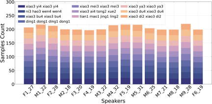
Fig. 3. Distribution of the evaluation corpus in the self-prepared Mandarin dataset. The horizontal axis shows the speaker’s ID marked by “Gender_Age.” Each keyword consists of four Chinese characters in pinyin format, as shown in the legend.
5.2.3. Background Noise Dataset
Additionally, noise samples were prepared for classification and augmentation. These samples were randomly extracted from the TUT Acoustic Scenes 2017 dataset 47. After constraining the volume levels to the range of \(-\)50 dB to \(-\)20 dB, we collected 10,000 and 7,064 background noise samples for augmentation and classification, respectively.
5.3. Evaluation Processes
In this section, we compare two related works with the proposed method, the CRNN-CTC method 6 and the few-shot classification method 40, which are referred to as CCKWS and FsKWS, respectively.
5.3.1. CRNN-CTC
CCKWS 6 trained a CRNN with connectionist temporal classification (CRNN-CTC) loss to produce frame-level acoustic embedding. The model was subsequently deployed as a feature extractor for QbE-KWS via dynamic time warping (DTW). It has two phases:
-
1.
Pretraining phase
-
2.
Evaluation phase
In the pretraining phase, the pretraining corpus was used to train the CRNN-CTC model. Character-level CTC targets were constructed by mapping each keyword string to a sequence of character indices drawn from predefined letters.
In the evaluation phase, the evaluation corpus was used for a 3-shot QbE evaluation. Specifically, for each keyword of the GSC, three samples were randomly selected as enrollment samples, while the remaining samples of the same keyword were positive samples and all the samples of other keywords were negative samples. The 150 SMD groups (speakers and keywords) were individually evaluated. For each group, three samples were used for enrollment; the remaining same-group samples served as positive samples, and all samples from all other groups constituted negative samples. The frame-level CRNN-CTC embeddings of the enrolled samples were first averaged into a query template, and the DTW distance between the template and each candidate sample was computed.
5.3.2. Few-Shot Classification
FsKWS 40 adopted a three-stage learning strategy:
-
1.
Pretraining phase
-
2.
Fine-tuning phase
-
3.
Evaluation phase
In the pretraining phase, the pretraining corpus was used to train the EfficientNet-B0 backbone as a multiclass-embedding model.
In the fine-tuning phase, a lightweight classification head is fine-tuned per keyword using augmented few-shot data to yield a 3-class model (target/canonical/noise). For each target keyword (10 held-out keywords for the GSC and 150 speaker-keyword combinations for the SMD), a 3-class few-shot training set was constructed. Specifically, 450 target samples were generated for training by augmenting the three enrollment samples using the augment module \(\mathcal{A}\). The remaining samples of the same keyword (after excluding the three enrollment samples) were split at \(6:4\) and augmented to complete 200 validations and 200 tests. Canonical samples were drawn from all remaining keywords (all other held-out keywords for GSC; all other speaker-keyword groups for Mandarin), randomly sampled to a pool of 850, and then split at \(450:200:200\) for training, validation, and testing. The noise class samples were randomly drawn from the classification subset of the background noise dataset (7,064 samples in total) and split at \(450:200:200\) for training, validation, and testing.
Consequently, the training, validation, and test sets used for training classification head \(\mathcal{C}\) consisted of 1,350, 600, and 600 samples, respectively. The datasets for the fine-tuning phase are shown in Fig. 4. All the samples were augmented using module \(\mathcal{A}\). The noise samples used for augmentation were obtained from the augmentation subset of the background noise dataset (10,000 samples in total).
In the evaluation phase, the 3-class model was used as the customized KWS model and was evaluated using a specific keyword. Specifically, for the GSC, each of the 10 customized models was evaluated against the keyword’s own test split. For the SMD, each of the 150 speaker-keyword models was evaluated based on its respective (speaker, keyword) test splits.
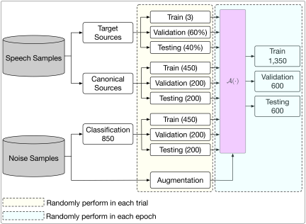
Fig. 4. The datasets for the fine-tuning phase of FsKWS and the proposed method.
5.3.3. Proposed Method
The CKWS method proposed in Section 4 followed a three-stage paradigm identical to that of FsKWS but replaced the EfficientNet-B0 backbone with CxLSTM.
5.4. Hyper-Parameters and Results
For CCKWS and FsKWS, all WAV samples from the GSC and SMD datasets were converted into 40-dimensional log-mel spectrograms as acoustic features. In contrast, the proposed CKWS model adopts a dual-stream input structure for the CxLSTM module, where a 128-dimensional log-mel spectrogram and a 32-dimensional MFCC feature are extracted simultaneously as two separate input branches. Moreover, for the classification head \(\mathcal{C}\) of our CKWS framework, the first dense layer was configured with 128 hidden units and equipped with a tanh activation function.
The fine-tuning phase of FsKWS and the proposed CKWS method consisted of 10 independent trials, each running for five training epochs. In each trial, the 3-class sources were randomly drawn once, whereas in each epoch, data augmentation was performed on all datasets, as shown in Fig. 4. A dropout layer with a probability of 0.5 was inserted during fine-tuning to mitigate overfitting. The mini-batch size was fixed at 8, and a multistep learning rate decay strategy was adopted; when the training steps reached 300, 600, and 840, the learning rate was adjusted to 0.001, 0.0005, and 0.0001, respectively.
In each trial, the training set was used to train the model, and the validation set was used to monitor the convergence of the model during training. When the model achieved the lowest loss value on the validation set, the performance on the test set was reported as the result of this trial. Finally, the results of the 10 trials are averaged in Table 2.
The results in Table 2 demonstrate the effectiveness of both the proposed CKWS and FsKWS methods, with FsKWS achieving a slightly superior performance on the GSC dataset. We attribute this outcome to the fact that FsKWS, which is built on the EfficientNet backbone, has a considerably larger parameter scale (Table 1), thereby enhancing the feature extraction capability. Consequently, FsKWS exhibited a better performance in the offline evaluation setting, where no resource constraints or background noise were imposed. In the following section, we compare the performances of these methods under real-world test scenarios.
6. Real-World Testing
In this section, the proposed CKWS method was deployed on Android and STM32 devices for evaluation in three real-world scenarios: living room, bedroom, and in-vehicle. All modules, including the asymmetric int8 quantized CxLSTM (module \(\mathcal{M}\)) and modules \(\mathcal{A}\) and \(\mathcal{C}\), were implemented in C. Additionally, we compared the results with those of the CCKWS and FsKWS.
6.1. Metrics
In real-world testing, we consider three metrics to evaluate the performance:
-
1.
Wake-up rate
-
2.
False alarm
-
3.
Latency
The wake-up rate refers to the percentage of times that the device successfully wakes up when the user says the target keyword. This metric measures the ability to recognize target keywords correctly. We recorded the number of times the device responded correctly out of 200 valid wake-up attempts.
A false alarm refers to the number of times a device is activated by nontarget sounds (such as daily conversations, environmental noise, or irrelevant words) over a certain period. Lower false alarms indicate better anti-interference performance. We recorded the number of false alarms every 24 h.
The latency indicates the time interval from when the user finishes saying the keyword to when the device starts responding. Lower latency enhances the user experience.
6.2. Enrollment and Evaluation Processes
We only tested the customization performance of Mandarin keywords in real-world scenarios and adopted identical keyword enrollment and evaluation pipelines for the CCKWS, FsKWS, and proposed CKWS methods. Specifically, we recruited four volunteers (two males and two females) to customize eight Mandarin keywords. Each volunteer customized two keywords according to their personal preferences, and only three recordings (3-shot) were required as enrollment samples for each keyword, with each recording having a duration of 2.5 s. All keywords were 4-character Chinese words, which is the mainstream format in the current market.
Note that the CCKWS only required these three samples to complete enrollment. In contrast, FsKWS and our proposed CKWS method additionally required a fine-tuning phase, in which the three enrollment samples were seen as the target sources. The evaluation corpus described in Section 5.2.2, consisting of 3,497 Mandarin recordings and 7,064 background noise samples, was prepared in advance as canonical sources and noise samples, respectively. In line with the dataset preparation shown in Fig. 4 and the hyperparameters detailed in Section 5.4, FsKWS and our proposed CKWS method accomplished keyword customization of the device.
During the wake-up test for a specific keyword, 200 prerecorded speech samples from volunteers were played using a playback source (loudspeaker) in both quiet and noisy environments. The false alarm test followed a similar protocol. Once the false-alarm test started, the microphone continuously captured an audio stream, and an inference process was executed every 0.5 s simultaneously. If a wake-up event was detected (i.e., the probability predicted as the target keyword exceeded the preset threshold), it was recorded as a false-alarm event.
6.3. Testing Environments
In the experiments, the sound level was measured by a sound level meter and quantified using the standard A-weighted sound pressure level dBA, with a unified reference sound pressure of (20 μPa) for airborne acoustic measurement. Under this international standard definition, 0 dBA represents the human auditory threshold of a 1 kHz pure tone.
In addition, we measured the reverberation time using a Room EQ Wizard (REW)(1) on a MacBook. Specifically, a loudspeaker generated swept signals to excite the room, and a MacBook microphone recorded impulse responses. In REW, the RT30 was calculated by fitting the \(-\)5 dB to \(-\)35 dB decay segment as the evaluation metric. In each real-world scenario, three measurement points were set with standardized placement heights and boundary distances, and each point was measured three times for averaging purposes.
We performed practical testing in three real-world scenarios: living room, bedroom, and in-vehicle environment. As illustrated in the bottom panel of Fig. 5, the living room has a rectangular layout with an area of approximately 36 square meters, measuring 9 m in length and 4 m in width. The device embedded with the test algorithm was placed 1 m from the long-side wall and 4.5 m from the short-side wall. A sound level meter and a MacBook were positioned near the device, through which we respectively measured a background noise level of around \(48{\pm}5\) dBA and a reverberation time of approximately 0.67 s.
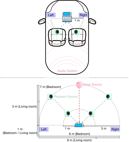
Fig. 5. The positions of the sources in the BYD car (top), the living room (bottom, \(4~\mathrm{m}\times 9~\mathrm{m}\)), and bedroom (bottom, \(8~\mathrm{m}\times 6~\mathrm{m}\)). The noise sources are not illustrated in the car since we do not know their exact positions.
The bedroom occupied an area of approximately 48 square meters (8 m long and 6 m wide). The device was placed 3 m from the long-side wall and 1 m from the short-side wall, as shown in the bottom panel of Fig. 5. The background noise level near the device was roughly \(45{\pm}5\) dBA, with a reverberation time of 0.63 s.
The in-vehicle environment was a more complex, irregular, enclosed space with an effective volume of approximately 5 cubic meters (we used a BYD Qin Plus car(2)). The device was placed close to the center console to guarantee acoustic conditions similar to those of the center console, as shown in the top panel of Fig. 5. When the vehicle remained parked, the background noise level near the device was approximately \(45{\pm}5\) dBA, and the reverberation time was 0.08 s.
In the wake-up test of the living room and bedroom, the device was positioned such that the playback source was aligned in two angular orientations relative to the center: 45° left and 45° right. Additionally, the distance between the playback source and device was set to two different values: 1 m and 3 m. To simulate a noisy environment, a noise source (another loudspeaker) was used for daily noise sampling.(3) It was fixed in a frontal position (0°) and maintained at a constant distance of 3 m from the device. This noise source configuration was consistently adopted in false alarm tests, with the key difference being that no playback source was deployed.
For the in-vehicle environment, two playback sources were placed on the driver and passenger seats. The device was positioned near the center console, 1 m from the playback sources at a 45° angular orientation. When a noisy environment was required, the audio system (consisting of six loudspeakers) of the BYD car was used directly to play the noise samples.(4)
6.4. Testing Platforms
We considered Android and STM32 devices as testing platforms. The Android device was a Redmi K60 smartphone equipped with an 8 GHz CPU and no GPU, with 8 GB of RAM. The selected STM32 hardware was a 32F746GDISCOVERY Discovery Kit(5) featuring an Arm Cortex-M7 core, 1 MB of flash memory, and 8 MB of SDRAM.
We deployed FsKWS and our proposed CKWS method on Android devices for testing in a bedroom. In the in-vehicle scenario, the proposed CKWS algorithm running on an Android device was directly compared with a native voice assistant system built into the center console. To the best of our knowledge, this center console has adopted the KWS engine developed by iFlytek,(6) which we refer to as iFKWS throughout this study. Finally, we implemented the proposed CKWS and CCKWS on an STM32 device and conducted tests in a living room.
The iFKWS and FsKWS methods were not deployed on the STM32 platform in this study for two reasons. First, the iFKWS is a highly customized commercial product developed in collaboration between iFlytek and BYD, and its source code is not publicly available. Second, as listed in Table 1, the EfficientNet-based FsKWS method contains 13M parameters, which requires approximately 49.6 MB of storage when stored in a 32-bit floating-point format. This requirement exceeds that of our selected STM32 device (1 MB flash memory). Consequently, neither method can be deployed on the STM32 platform.
It is worth noting that FsKWS, CCKWS, and the proposed CKWS fall into the category of QbE methods that require users to record speech samples for enrollment. By contrast, iFKWS adopts the QbS paradigm, in which users customize keywords by merely inputting text strings rather than recording enrollment samples. The hardware devices adopted for each test scenario are summarized in Table 3. It can be found that our experiments covered three mainstream scenarios and two typical hardware platforms, which comprehensively verified the robustness and effectiveness of the proposed CKWS under diverse computational resource constraints and acoustic environments.
6.5. Testing Results
The test results in three scenarios with a preset threshold of 0.9 are summarized in Tables 4, 5, and 6 in Appendix A, respectively. In the tables, the “noise level” refers to the sound level measured at the device when only the noise source is present in the environment. In contrast, the “record level” refers to the sound level measured at the device under the corresponding test environment (quiet or noisy environment). The average wake-up rate results in “Noisy” and “Quiet” representing the environment with and without the noise source, respectively.
As can be observed from the results presented in Table 5, FsKWS exhibited a higher wake-up sensitivity, which contributed to its high wake-up rate but also led to a large number of false alarms. In contrast, the iFKWS had a lower wake-up sensitivity, resulting in good false alarm performance but a relatively low wake-up rate, as shown in Table 6. Similar observations can be made for the CCKWS case, as shown in Table 4. However, the CCKWS achieved a slightly lower latency than the proposed method, which may be attributed to its lower memory occupation, as shown in Table 1. In summary, the method proposed in this study achieved a favorable false-alarm performance while maintaining a high wake-up rate. Additionally, the average latency was significantly lower than that of the FsKWS method, demonstrating the high efficiency of the proposed method.
7. Discussion
7.1. Model Quantization
We opted for asymmetric int8 quantization despite its higher reconstruction error (MAE) compared with int16 because it halves the storage footprint, which is a critical advantage for edge deployment. Crucially, our experimental results indicate that the performance degradation caused by quantization is effectively mitigated by data augmentation strategy (\(\mathcal{A}\)), which enhances the model robustness against feature perturbations. This suggests a synergistic relationship between quantization and augmentation. The latter acts as a regularizer, compensating for the approximation error of the former.
Although the proposed CKWS method achieved better performance than the CCKWS method, as shown in Tables 2 and 4, the memory occupation was slightly larger than that of CCKWS, which resulted in a higher latency. In future work, we plan to explore static quantization and quantization-aware training (QAT) to further reduce memory occupation while minimizing performance degradation.
7.2. False Alarm
Although our method achieved a low false alarm rate under controlled testing, real-world deployment may reveal greater susceptibility to environmental noise and overlapping speech. This limitation stems from the current simple logic: the wake-up result is determined solely based on the output probability of the current frame. These frame-level decisions are inherently coarse and sensitive to transient acoustic events. To address this, we plan to integrate a temporal filtering mechanism. For instance, a wake-up event would only be confirmed if multiple consecutive frames exhibit high probabilities that follow an increasing trend. Additionally, implementing a “Cool-Down Period” (e.g., 2–3 s) after a successful wake-up could further reduce false alarms, which would prevent repeated triggering from reverberation or user repetition.
8. Conclusions
This paper presents CxLSTM, an efficient module for CKWS on edge devices. Through dynamic quantization, CxLSTM achieves a small memory footprint and low computational cost, making it highly suitable for edge deployment. Building upon CxLSTM, we propose a modular online customization pipeline to achieve rapid CKWS with minimal overhead. Comprehensive experiments in both offline and real-world scenarios demonstrate the efficacy of the proposed approach. Future work will focus on advancing quantization techniques and temporal decision logic to improve performance.
Acknowledgments
H. Cao acknowledges Qihui Feng for his review and discussion on this paper. All authors thank the volunteers from Guangzhou Polytechnic University. This research was funded in part by the Higher Education Scientific Research Project of the Guangzhou Municipal Education Bureau under Grant 2024312335, the Collaborative Innovation Center for Intelligent Educational Technology of Guangzhou under Grants 2023B04J0004 and 2025B04J0007, the Key Research Platform of Guangzhou Polytechnic University under Grant 2026KYPT01, the Scientific Research Project of the Education Department of Guangdong under Grant 2022ZDZX1065, 2023ZDZX1072, 2025ZDZX1056.
Footnotes
(1) Room EQ Wizard: https://www.roomeqwizard.com/ [Accessed June 20, 2026]
(2) Car model: https://www.byd.com/cn/dynasty-home/models/qin/26-qin-l-dm-i [Accessed October 10, 2025]
(3) Around 36 hours of noise data coming from the evaluation dataset of the DECASE 2019 TASK 4 48, including 10 classes of sound events: speech, dog, cat, alarm/bell/ringing, dishes, frying, blender, running water, vacuum clearner, electric shaver/toothbrush in domestic environments.
(4) Around 20 hours of music, TV shows, cartoons, and radio broadcasts downloaded from the Internet.
(5) 32F746GDISCOVERY Discovery kit: https://www.st.com/en/evaluation-tools/32f746gdiscovery.html [Accessed October 21, 2025]
(6) iFLYTEK CO.LTD.: http://www.iflyauto.com/interact [Accessed October 21, 2025]
- [1] O. Friha, M. A. Ferrag, B. Kantarci, B. Cakmak, A. Ozgun, and N. Ghoualmi-Zine, “Llm-based edge intelligence: A comprehensive survey on architectures, applications, security and trustworthiness,” IEEE Open J. of the Communications Society, Vol.5, pp. 5799-5856, 2024. https://doi.org/10.1109/OJCOMS.2024.3456549
- [2] S. Anusha, M. Ezhilvandan, S. Gayathri, V. Sivaraman et al., “Emerging trends in edge AI for Industry 4.0 and 5.0: Technologies, applications, and challenges,” AI Innovations in Service and Tourism Marketing, pp. 211-228, 2024. https://doi.org/10.4018/979-8-3693-7909-7.ch010
- [3] Y. Sone and J. Woo, “Design of a Human-Centric Robotic System for User Support Based on Gaze Information,” J. Adv. Comput. Intell. Intell. Inform., Vol.29, No.4, pp. 796-802, 2025. https://doi.org/10.20965/jaciii.2025.p0796
- [4] Z. Zhang, R. Li, and K. Chen, “A Parallel CNN-Transformer Framework for Speech Age Recognition,” J. Adv. Comput. Intell. Intell. Inform., Vol.29, No.5, pp. 1137-1144, 2025. https://doi.org/10.20965/jaciii.2025.p1137
- [5] C. Mao and S. Liu, “A Study on Speech Recognition by a Neural Network Based on English Speech Feature Parameters,” J. Adv. Comput. Intell. Intell. Inform., Vol.28, No.3, pp. 679-684, 2024. https://doi.org/10.20965/jaciii.2024.p0679
- [6] M. Li, “A Lightweight Architecture for Query-by-Example Keyword Spotting on Low-Power IoT Devices,” IEEE Trans. on Consumer Electronics, Vol.69, No.1, pp. 65-75, 2023. https://doi.org/10.1109/TCE.2022.3213075
- [7] Y. Wei, Z. Gong, S. Yang, K. Ye, and Y. Wen, “EdgeCRNN: an edge-computing oriented model of acoustic feature enhancement for keyword spotting,” J. of Ambient Intelligence and Humanized Computing, Vol.13, No.3, pp. 1525-1535, 2022. https://doi.org/10.1007/s12652-021-03022-1
- [8] L. Lei, G. Yuan, H. Yu, D. Kong, and Y. He, “Multilingual Customized Keyword Spotting Using Similar-Pair Contrastive Learning,” IEEE/ACM Trans. on Audio, Speech, and Language Processing, Vol.31, pp. 2437-2447, 2023. https://doi.org/10.1109/TASLP.2023.3284523
- [9] M. Rusci and T. Tuytelaars, “Few-Shot Open-Set Learning for On-Device Customization of KeyWord Spotting Systems,” Interspeech 2023, pp. 2768-2772, 2023. https://doi.org/10.21437/Interspeech.2023-1904
- [10] Q. Shao, J. Hou, Y. Hu, Q. Wang, L. Xie, and X. Lei, “Target speaker extraction for customizable query-by-example keyword spotting,” 2021 Asia-Pacific Signal and Information Processing Association Annual Summit and Conf. (APSIPA ASC), pp. 672-678, 2021.
- [11] Z. Yang, S. Sun, J. Li, X. Zhang, X. Wang, L. Ma, and L. Xie, “CaTT-KWS: A Multi-stage Customized Keyword Spotting Framework based on Cascaded Transducer-Transformer,” Interspeech 2022, pp. 1681-1685, 2022. https://doi.org/10.21437/Interspeech.2022-10258
- [12] H. Yan, Q. He, and W. Xie, “CRNN-CTC based mandarin keywords spotting,” ICASSP 2020-2020 IEEE Int. Conf. on Acoustics, Speech and Signal Processing (ICASSP), pp. 7489-7493, 2020. https://doi.org/10.1109/ICASSP40776.2020.9054618
- [13] S. Li and H. Zhang, “Keyword spotting based on CTC and Similarity Matching for Chinese Speech,” 2023 IEEE/ACIS 23rd Int. Conf. on Computer and Information Science (ICIS), pp. 79-84, 2023. https://doi.org/10.1109/ICIS57766.2023.10210227
- [14] T. N. Sainath and C. Parada, “Convolutional neural networks for small-footprint keyword spotting,” Interspeech 2015, pp. 1478-1482, 2015. https://doi.org/10.21437/Interspeech.2015-352
- [15] G. Chen, C. Parada, and T. N. Sainath, “Query-by-example keyword spotting using long short-term memory networks,” 2015 IEEE Int. Conf. on Acoustics, Speech and Signal Processing (ICASSP), pp. 5236-5240, 2015. https://doi.org/10.1109/ICASSP.2015.7178970
- [16] S. Ö. Arik, M. Kliegl, R. Child, J. Hestness, A. Gibiansky, C. Fougner, R. Prenger, and A. Coates, “Convolutional Recurrent Neural Networks for Small-Footprint Keyword Spotting,” Interspeech 2017, pp. 1606-1610, 2017. https://doi.org/10.21437/Interspeech.2017-1737
- [17] S. Majumdar and B. Ginsburg, “MatchboxNet: 1D Time-Channel Separable Convolutional Neural Network Architecture for Speech Commands Recognition,” Interspeech 2020, pp. 3356-3360, 2020. https://doi.org/10.21437/Interspeech.2020-1058
- [18] B. Kim, S. Chang, J. Lee, and D. Sung, “Broadcasted Residual Learning for Efficient Keyword Spotting,” Interspeech 2021, pp. 4538-4542, 2021. https://doi.org/10.21437/Interspeech.2021-383
- [19] S. Choi, S. Seo, B. Shin, H. Byun, M. Kersner, B. Kim, D. Kim, and S. Ha, “Temporal Convolution for Real-Time Keyword Spotting on Mobile Devices,” Interspeech 2019, pp. 3372-3376, 2019. https://doi.org/10.21437/Interspeech.2019-1363
- [20] J. Huang, W. Gharbieh, Q. Wan, H. S. Shim, and H. C. Lee, “QbyE-MLPMixer: Query-by-Example Open-Vocabulary Keyword Spotting using MLPMixer,” Interspeech 2022, pp. 5200-5204, 2022. https://doi.org/10.21437/Interspeech.2022-11080
- [21] A. Vaswani, N. Shazeer, N. Parmar, J. Uszkoreit, L. Jones, A. N. Gomez, Ł. Kaiser, and I. Polosukhin, “Attention is all you need,” Advances in Neural Information Processing Systems, pp. 6000-6010, 2017.
- [22] A. Berg, M. O’Connor, and M. T. Cruz, “Keyword Transformer: A Self-Attention Model for Keyword Spotting,” Interspeech 2021, pp. 4249-4253, 2021. https://doi.org/10.21437/Interspeech.2021-1286
- [23] K. Ding, M. Zong, J. Li, and B. Li, “LETR: A Lightweight and Efficient Transformer for Keyword Spotting,” 2022 IEEE Int. Conf. on Acoustics, Speech and Signal Processing (ICASSP), pp. 7987-7991, 2022. https://doi.org/10.1109/ICASSP43922.2022.9747295
- [24] N. Kitaev, Ł. Kaiser, and A. Levskaya, “Reformer: The efficient transformer,” arXiv preprint, arXiv:2001.04451, 2020. https://doi.org/10.48550/arXiv.2001.04451
- [25] Y. Li, G. Yuan, Y. Wen, J. Hu, G. Evangelidis, S. Tulyakov, Y. Wang, and J. Ren, “EfficientFormer: Vision Transformers at MobileNet Speed,” Advances in Neural Information Processing Systems, Vol.35, pp. 12934-12949, 2022. https://doi.org/10.52202/068431-0940
- [26] M. Beck, K. Pöppel, M. Spanring, A. Auer, O. Prudnikova, M. Kopp, G. Klambauer, J. Brandstetter, and S. Hochreiter, “xLSTM: Extended Long Short-Term Memory,” Advances in Neural Information Processing Systems, Vol.37, pp. 107547-107603, 2024. https://doi.org/10.52202/079017-3417
- [27] S. Yadav, S. Theodoridis, and Z.-H. Tan, “AxLSTMs: learning self-supervised audio representations with xLSTMs,” Interspeech 2025, pp. 3524-3528, 2025. https://doi.org/10.21437/Interspeech.2025-426
- [28] B. Alkin, M. Beck, K. Pöppel, S. Hochreiter, and J. Brandstetter, “Vision-LSTM: xLSTM as Generic Vision Backbone,” The Thirteenth Int. Conf. on Learning Representations, 2025.
- [29] Z. Liu, T. Li, and P. Zhang, “RNN-T based open-vocabulary keyword spotting in mandarin with multi-level detection,” 2021 IEEE Int. Conf. on Acoustics, Speech and Signal Processing (ICASSP), pp. 5649-5653, 2021. https://doi.org/10.1109/ICASSP39728.2021.9413588
- [30] S.-G. Leem, I.-C. Yoo, and D. Yook, “Multitask Learning of Deep Neural Network-Based Keyword Spotting for IoT Devices,” IEEE Trans. on Consumer Electronics, Vol.65, No.2, pp. 188-194, 2019. https://doi.org/10.1109/TCE.2019.2899067
- [31] E. van der Westhuizen, H. Kamper, R. Menon, J. Quinn, and T. Niesler, “Feature learning for efficient ASR-free keyword spotting in low-resource languages,” Computer Speech & Language, Vol.71, Article No.101275, 2022. https://doi.org/10.1016/j.csl.2021.101275
- [32] K. R, V. K. Kurmi, V. Namboodiri, and C. V. Jawahar, “Generalized Keyword Spotting using ASR embeddings,” Interspeech 2022, pp. 126-130, 2022. https://doi.org/10.21437/Interspeech.2022-10450
- [33] Y. Yang, B. Du, Y. Zhang, W. Wang, and Y. Li, “BBS-KWS: The Mandarin Keyword Spotting System Won the Video Keyword Wakeup Challenge,” arXiv preprint, arXiv:2112.01757, 2021. https://doi.org/10.48550/arXiv.2112.01757
- [34] E. T. Mekonnen, A. Brutti, and D. Falavigna, “End-to-end low resource keyword spotting through character recognition and beam-search re-scoring,” 2022 IEEE Int. Conf. on Acoustics, Speech and Signal Processing (ICASSP), pp. 8182-8186, 2022. https://doi.org/10.1109/ICASSP43922.2022.9746012
- [35] B. Labrador, G. Zhao, I. L. Moreno, A. S. Scarpati, L. Fowl, and Q. Wang, “Exploring Sequence-to-Sequence Transformer-Transducer Models for Keyword Spotting,” 2023 IEEE Int. Conf. on Acoustics, Speech and Signal Processing (ICASSP), 2023. https://doi.org/10.17023/r23c-4m17
- [36] A. Parnami and M. Lee, “Few-Shot Keyword Spotting With Prototypical Networks,” Proc. of the 2022 7th Int. Conf. on Machine Learning Technologies (ICMLT ’22), pp. 277-283, 2022. https://doi.org/10.1145/3529399.3529443
- [37] J. Lin, K. Kilgour, D. Roblek, and M. Sharifi, “Training keyword spotters with limited and synthesized speech data,” 2020 IEEE Int. Conf. on Acoustics, Speech and Signal Processing (ICASSP), pp. 7474-7478, 2020. https://doi.org/10.1109/ICASSP40776.2020.9053193
- [38] M. Xu and X.-L. Zhang, “Depthwise Separable Convolutional ResNet with Squeeze-and-Excitation Blocks for Small-Footprint Keyword Spotting,” Interspeech 2020, pp. 2547-2551, 2020. https://doi.org/10.21437/Interspeech.2020-1045
- [39] M. Sun, A. Raju, G. Tucker, S. Panchapagesan, G. Fu, A. Mandal, S. Matsoukas, N. Strom, and S. Vitaladevuni, “Max-pooling loss training of long short-term memory networks for small-footprint keyword spotting,” 2016 IEEE Spoken Language Technology Workshop (SLT), pp. 474-480, 2016. https://doi.org/10.1109/SLT.2016.7846306
- [40] M. Mazumder, C. Banbury, J. Meyer, P. Warden, and V. J. Reddi, “Few-Shot Keyword Spotting in Any Language,” Interspeech 2021, pp. 4214-4218, 2021. https://doi.org/10.21437/Interspeech.2021-1966
- [41] Y. Xi, T. Tan, W. Zhang, B. Yang, and K. Yu, “Text adaptive detection for customizable keyword spotting,” 2022 IEEE Int. Conf. on Acoustics, Speech and Signal Processing (ICASSP), pp. 6652-6656, 2022. https://doi.org/10.1109/ICASSP43922.2022.9746647
- [42] B. Wei, M. Yang, T. Zhang, X. Tang, X. Huang, K. Kim, J. Lee, K. Cho, and S.-U. Park, “End-to-End Transformer-Based Open-Vocabulary Keyword Spotting with Location-Guided Local Attention,” Interspeech 2021, pp. 361-365, 2021. https://doi.org/10.21437/Interspeech.2021-1335
- [43] H. Cao, X. Liu, Z. Tan, Z. Yang, and X. Qin, “Custom Mandarin Keyword Spotting with Extended Long Short-Term Memory,” IAENG Int. J. of Computer Science, Vol.51, No.12, Article No.1933, 2024.
- [44] D. S. Park, W. Chan, Y. Zhang, C.-C. Chiu, B. Zoph, E. D. Cubuk, and Q. V. Le, “SpecAugment: A Simple Data Augmentation Method for Automatic Speech Recognition,” Interspeech 2019, pp. 2613-2617, 2019. https://doi.org/10.21437/Interspeech.2019-2680
- [45] T. Devries and G. W. Taylor, “Improved Regularization of Convolutional Neural Networks with Cutout,” arXiv preprint, arXiv:1708.04552, 2017. https://doi.org/10.48550/arXiv.1708.04552
- [46] P. Warden, “Speech commands: A dataset for limited-vocabulary speech recognition,” arXiv preprint, arXiv:1804.03209, 2018. https://doi.org/10.48550/arXiv.1804.03209
- [47] A. Mesaros, T. Heittola, A. Diment, B. Elizalde, A. Shah, E. Vincent, B. Raj, and T. Virtanen, “DCASE 2017 Challenge Setup: Tasks, Datasets and Baseline System,” Proc. of the Detection and Classification of Acoustic Scenes and Events 2017 Workshop (DCASE2017), pp. 85-92, 2017.
- [48] N. Turpault, R. Serizel, A. P. Shah, and J. Salamon, “Sound event detection in domestic environments with weakly labeled data and soundscape synthesis,” Workshop on Detection and Classification of Acoustic Scenes and Events, 2019. https://doi.org/10.33682/006b-jx26
Appendix
Appendix A. Test Results of the Real-World Testing
We conducted real-world evaluations in three practical scenarios: a living room, a bedroom, and a vehicle. The proposed method was benchmarked against three existing approaches, namely CCKWS, FsKWS, and iFKWS. The corresponding experimental results are summarized in Tables 4, 5, and 6.
| Speaker | Keyword | Test environment | Wake-up rate [%] | False alarm (/24 h) | Latency [ms] | ||||||
| Playback source | Environmental levels [dBA] | ||||||||||
| Distance | Angle | Noise | Record | CCKWS | Ours | CCKWS | Ours | CCKWS | Ours | ||
| \(P_1\) | nai3 cha2 bu4 ding1 | 1m | Left 45° | 55\(\pm\)5 | 60\(\pm\)5 | 88.0 | 92.5 | – | 249.3 | 283.4 | |
| Right 45° | 89.0 | 94.0 | – | 267.3 | 273.3 | ||||||
| Left 45° | – | 48\(\pm\)5 | 89.5 | 94.0 | – | 234.1 | 274.3 | ||||
| Right 45° | 93.0 | 94.0 | – | 237.8 | 285.1 | ||||||
| 3m | Left 45° | 55\(\pm\)5 | 60\(\pm\)5 | 86.5 | 92.5 | – | 253.7 | 294.6 | |||
| Right 45° | 87.0 | 90.5 | – | 246.1 | 274.5 | ||||||
| Left 45° | – | 48\(\pm\)5 | 93.0 | 95.5 | – | 266.3 | 273.5 | ||||
| Right 45° | 92.0 | 94.5 | – | 273.6 | 294.5 | ||||||
| – | 55\(\pm\)5 | 55\(\pm\)5 | – | 14 | 16 | – | |||||
| \(P_1\) | a1 wen2 tong2 xue2 | 1m | Left 45° | 55\(\pm\)5 | 60\(\pm\)5 | 85.5 | 92.5 | – | 246.3 | 274.6 | |
| Right 45° | 88.5 | 90.5 | – | 254.4 | 275.3 | ||||||
| Left 45° | – | 48\(\pm\)5 | 93.0 | 94.5 | – | 254.6 | 264.3 | ||||
| Right 45° | 92.0 | 94.5 | – | 246.5 | 257.3 | ||||||
| 3m | Left 45° | 55\(\pm\)5 | 60\(\pm\)5 | 89.0 | 90.5 | – | 235.4 | 264.6 | |||
| Right 45° | 88.5 | 92.5 | – | 245.3 | 264.6 | ||||||
| Left 45° | – | 48\(\pm\)5 | 93.0 | 94.5 | – | 244.5 | 263.5 | ||||
| Right 45° | 92.5 | 95.5 | – | 245.3 | 267.4 | ||||||
| – | 55\(\pm\)5 | 55\(\pm\)5 | – | 13 | 16 | – | |||||
| \(P_2\) | ni3 hao3 mu4 mu4 | 1m | Left 45° | 55\(\pm\)5 | 60\(\pm\)5 | 89.0 | 90.5 | – | 245.7 | 253.5 | |
| Right 45° | 89.0 | 94.0 | – | 237.4 | 256.7 | ||||||
| Left 45° | – | 48\(\pm\)5 | 91.5 | 90.5 | – | 249.3 | 253.4 | ||||
| Right 45° | 92.5 | 92.0 | – | 246.6 | 255.4 | ||||||
| 3m | Left 45° | 55\(\pm\)5 | 60\(\pm\)5 | 88.5 | 93.5 | – | 236.1 | 254.6 | |||
| Right 45° | 88.0 | 92.5 | – | 255.7 | 267.3 | ||||||
| Left 45° | – | 48\(\pm\)5 | 92.5 | 94.5 | – | 245.1 | 257.7 | ||||
| Right 45° | 92.5 | 95.5 | – | 244.2 | 257.5 | ||||||
| – | 55\(\pm\)5 | 55\(\pm\)5 | – | 14 | 15 | – | |||||
| \(P_2\) | ha1 lou1 she4 zhang3 | 1m | Left 45° | 55\(\pm\)5 | 60\(\pm\)5 | 89.0 | 92.5 | – | 249.5 | 255.7 | |
| Right 45° | 88.5 | 93.0 | – | 253.6 | 266.8 | ||||||
| Left 45° | – | 48\(\pm\)5 | 92.5 | 95.5 | – | 249.5 | 263.4 | ||||
| Right 45° | 93.5 | 94.5 | – | 259.3 | 267.1 | ||||||
| 3m | Left 45° | 55\(\pm\)5 | 60\(\pm\)5 | 84.5 | 90.5 | – | 248.5 | 265.3 | |||
| Right 45° | 87.0 | 89.5 | – | 246.3 | 259.7 | ||||||
| Left 45° | – | 48\(\pm\)5 | 92.0 | 94.5 | – | 255.6 | 275.3 | ||||
| Right 45° | 93.0 | 94.0 | – | 258.3 | 265.6 | ||||||
| – | 55\(\pm\)5 | 55\(\pm\)5 | – | 17 | 20 | – | |||||
| \(P_3\) | ni3 hao3 xiao3 xin1 | 1m | Left 45° | 55\(\pm\)5 | 60\(\pm\)5 | 89.0 | 92.5 | – | 249.5 | 254.6 | |
| Right 45° | 88.0 | 93.5 | – | 255.8 | 265.7 | ||||||
| Left 45° | – | 48\(\pm\)5 | 93.0 | 94.5 | – | 258.8 | 264.7 | ||||
| Right 45° | 92.5 | 92.5 | – | 254.7 | 265.4 | ||||||
| 3m | Left 45° | 55\(\pm\)5 | 60\(\pm\)5 | 88.5 | 92.0 | – | 244.7 | 248.5 | |||
| Right 45° | 89.0 | 93.5 | – | 253.6 | 267.4 | ||||||
| Left 45° | – | 48\(\pm\)5 | 92.0 | 95.0 | – | 257.7 | 261.5 | ||||
| Right 45° | 91.0 | 94.5 | – | 259.3 | 263.2 | ||||||
| – | 55\(\pm\)5 | 55\(\pm\)5 | – | 18 | 16 | – | |||||
| \(P_3\) | xiao3 huang2 zai4 ma1 | 1m | Left 45° | 55\(\pm\)5 | 60\(\pm\)5 | 87.0 | 92.5 | – | 256.7 | 274.5 | |
| Right 45° | 87.0 | 92.0 | – | 257.7 | 264.3 | ||||||
| Left 45° | – | 48\(\pm\)5 | 92.5 | 94.5 | – | 253.8 | 267.4 | ||||
| Right 45° | 90.0 | 94.5 | – | 255.9 | 268.4 | ||||||
| 3m | Left 45° | 55\(\pm\)5 | 60\(\pm\)5 | 88.0 | 92.0 | – | 255.8 | 267.4 | |||
| Right 45° | 89.5 | 92.5 | – | 249.6 | 253.5 | ||||||
| Left 45° | – | 48\(\pm\)5 | 93.0 | 94.0 | – | 257.6 | 264.5 | ||||
| Right 45° | 92.0 | 94.5 | – | 255.3 | 265.4 | ||||||
| – | 55\(\pm\)5 | 55\(\pm\)5 | – | 10 | 12 | – | |||||
| \(P_4\) | tuan2 tuan2 guo4 lai2 | 1m | Left 45° | 55\(\pm\)5 | 60\(\pm\)5 | 88.0 | 92.5 | – | 259.4 | 266.4 | |
| Right 45° | 89.5 | 93.5 | – | 235.3 | 242.1 | ||||||
| Left 45° | – | 48\(\pm\)5 | 92.5 | 92.5 | – | 251.5 | 265.7 | ||||
| Right 45° | 91.5 | 94.5 | – | 255.7 | 261.3 | ||||||
| 3m | Left 45° | 55\(\pm\)5 | 60\(\pm\)5 | 88.0 | 92.5 | – | 254.6 | 258.4 | |||
| Right 45° | 89.0 | 93.5 | – | 255.3 | 264.5 | ||||||
| Left 45° | – | 48\(\pm\)5 | 91.5 | 94.5 | – | 256.3 | 259.4 | ||||
| Right 45° | 91.0 | 94.0 | – | 253.6 | 264.3 | ||||||
| – | 55\(\pm\)5 | 55\(\pm\)5 | – | 15 | 16 | – | |||||
| \(P_4\) | liu2 lian2 pi1 sa4 | 1m | Left 45° | 55\(\pm\)5 | 60\(\pm\)5 | 89.5 | 92.5 | – | 259.4 | 266.4 | |
| Right 45° | 86.5 | 92.0 | – | 259.6 | 267.1 | ||||||
| Left 45° | – | 48\(\pm\)5 | 92.0 | 92.0 | – | 259.6 | 264.4 | ||||
| Right 45° | 93.0 | 96.0 | – | 254.6 | 256.1 | ||||||
| 3m | Left 45° | 55\(\pm\)5 | 60\(\pm\)5 | 88.0 | 92.0 | – | 253.4 | 257.1 | |||
| Right 45° | 88.0 | 92.5 | – | 251.2 | 256.4 | ||||||
| Left 45° | – | 48\(\pm\)5 | 91.5 | 94.5 | – | 249.5 | 255.6 | ||||
| Right 45° | 93.5 | 92.5 | – | 252.8 | 256.7 | ||||||
| – | 55\(\pm\)5 | 55\(\pm\)5 | – | 13 | 15 | – | |||||
| Average | Noisy: 88.1 Quiet: 92.2 | Noisy: 92.3 Quiet: 94.1 | 14.3 | 15.8 | 251.9 | 264.7 | |||||
| Speaker | Keyword | Test environment | Wake-up rate [%] | False alarm (/24 h) | Latency [ms] | ||||||
| Playback source | Environmental levels [dBA] | ||||||||||
| Distance | Angle | Noise | Record | FsKWS | Ours | FsKWS | Ours | FsKWS | Ours | ||
| \(P_1\) | nai3 cha2 bu4 ding1 | 1m | Left 45° | 55\(\pm\)5 | 60\(\pm\)5 | 95.0 | 94.5 | – | 14.9 | 2.5 | |
| Right 45° | 99.0 | 94.5 | – | 14.9 | 4.1 | ||||||
| Left 45° | – | 45\(\pm\)5 | 97.5 | 97.0 | – | 14.9 | 1.4 | ||||
| Right 45° | 97.0 | 97.0 | – | 13.6 | 3.5 | ||||||
| 3m | Left 45° | 55\(\pm\)5 | 60\(\pm\)5 | 95.0 | 94.5 | – | 11.3 | 1.4 | |||
| Right 45° | 97.0 | 94.5 | – | 14.9 | 3.1 | ||||||
| Left 45° | – | 45\(\pm\)5 | 99.0 | 96.5 | – | 14.9 | 4.6 | ||||
| Right 45° | 96.0 | 97.0 | – | 14.9 | 1.4 | ||||||
| – | 55\(\pm\)5 | 55\(\pm\)5 | – | 12 | 2 | – | |||||
| \(P_1\) | a1 wen2 tong2 xue2 | 1m | Left 45° | 55\(\pm\)5 | 60\(\pm\)5 | 95.0 | 96.5 | – | 14.9 | 1.4 | |
| Right 45° | 95.5 | 94.5 | – | 10.3 | 1.4 | ||||||
| Left 45° | – | 45\(\pm\)5 | 96.5 | 97.5 | – | 14.6 | 1.4 | ||||
| Right 45° | 98.0 | 98.0 | – | 14.9 | 1.7 | ||||||
| 3m | Left 45° | 55\(\pm\)5 | 60\(\pm\)5 | 95.0 | 94.5 | – | 11.7 | 1.4 | |||
| Right 45° | 95.5 | 94.5 | – | 13.7 | 1.4 | ||||||
| Left 45° | – | 45\(\pm\)5 | 97.0 | 98.5 | – | 12.2 | 1.4 | ||||
| Right 45° | 97.5 | 96.5 | – | 14.9 | 1.4 | ||||||
| – | 55\(\pm\)5 | 55\(\pm\)5 | – | 15 | 1 | – | |||||
| \(P_2\) | ni3 hao3 mu4 mu4 | 1m | Left 45° | 55\(\pm\)5 | 60\(\pm\)5 | 95.0 | 94.5 | – | 13.2 | 1.4 | |
| Right 45° | 96.0 | 96.0 | – | 14.9 | 4.5 | ||||||
| Left 45° | – | 45\(\pm\)5 | 99.5 | 98.5 | – | 14.9 | 1.4 | ||||
| Right 45° | 97.5 | 98.0 | – | 12.6 | 1.4 | ||||||
| 3m | Left 45° | 55\(\pm\)5 | 60\(\pm\)5 | 97.5 | 95.5 | – | 12.3 | 3.2 | |||
| Right 45° | 95.0 | 96.5 | – | 14.0 | 1.4 | ||||||
| Left 45° | – | 45\(\pm\)5 | 99.5 | 98.5 | – | 9.1 | 1.4 | ||||
| Right 45° | 98.5 | 96.5 | – | 14.9 | 4.7 | ||||||
| – | 55\(\pm\)5 | 55\(\pm\)5 | – | 4 | 0 | – | |||||
| \(P_2\) | ha1 lou1 she4 zhang3 | 1m | Left 45° | 55\(\pm\)5 | 60\(\pm\)5 | 96.0 | 94.5 | – | 14.9 | 1.4 | |
| Right 45° | 96.5 | 95.0 | – | 13.5 | 1.4 | ||||||
| Left 45° | – | 45\(\pm\)5 | 99.5 | 97.5 | – | 14.9 | 1.4 | ||||
| Right 45° | 96.5 | 96.5 | – | 14.9 | 3.4 | ||||||
| 3m | Left 45° | 55\(\pm\)5 | 60\(\pm\)5 | 96.5 | 94.5 | – | 14.9 | 2.8 | |||
| Right 45° | 99.0 | 96.5 | – | 14.9 | 1.4 | ||||||
| Left 45° | – | 45\(\pm\)5 | 98.0 | 98.5 | – | 12.5 | 1.4 | ||||
| Right 45° | 97.0 | 98.0 | – | 14.8 | 2.1 | ||||||
| – | 55\(\pm\)5 | 55\(\pm\)5 | – | 13 | 0 | – | |||||
| \(P_3\) | ni3 hao3 xiao3 xin1 | 1m | Left 45° | 55\(\pm\)5 | 60\(\pm\)5 | 98.0 | 94.5 | – | 14.9 | 2.5 | |
| Right 45° | 97.0 | 94.5 | – | 14.9 | 2.4 | ||||||
| Left 45° | – | 45\(\pm\)5 | 98.0 | 96.5 | – | 14.9 | 1.4 | ||||
| Right 45° | 99.5 | 98.5 | – | 10.9 | 1.4 | ||||||
| 3m | Left 45° | 55\(\pm\)5 | 60\(\pm\)5 | 96.5 | 95.0 | – | 14.9 | 1.4 | |||
| Right 45° | 96.0 | 94.5 | – | 11.6 | 1.4 | ||||||
| Left 45° | – | 45\(\pm\)5 | 99.0 | 98.0 | – | 14.9 | 1.4 | ||||
| Right 45° | 98.0 | 97.5 | – | 14.9 | 1.7 | ||||||
| – | 55\(\pm\)5 | 55\(\pm\)5 | – | 22 | 1 | – | |||||
| \(P_3\) | xiao3 huang2 zai4 ma1 | 1m | Left 45° | 55\(\pm\)5 | 60\(\pm\)5 | 99.0 | 94.5 | – | 12.0 | 1.4 | |
| Right 45° | 95.0 | 96.5 | – | 14.9 | 2.8 | ||||||
| Left 45° | – | 45\(\pm\)5 | 99.5 | 96.5 | – | 14.9 | 1.4 | ||||
| Right 45° | 98.0 | 97.5 | – | 11.7 | 3.3 | ||||||
| 3m | Left 45° | 55\(\pm\)5 | 60\(\pm\)5 | 96.0 | 95.0 | – | 10.8 | 1.4 | |||
| Right 45° | 96.5 | 94.5 | – | 14.9 | 3.7 | ||||||
| Left 45° | – | 45\(\pm\)5 | 96.0 | 97.0 | – | 14.9 | 1.4 | ||||
| Right 45° | 96.0 | 98.0 | – | 14.9 | 1.4 | ||||||
| – | 55\(\pm\)5 | 55\(\pm\)5 | – | 5 | 0 | – | |||||
| \(P_4\) | tuan2 tuan2 guo4 lai2 | 1m | Left 45° | 55\(\pm\)5 | 60\(\pm\)5 | 95.0 | 95.5 | – | 14.9 | 1.4 | |
| Right 45° | 98.5 | 94.5 | – | 9.3 | 2.4 | ||||||
| Left 45° | – | 45\(\pm\)5 | 99.5 | 96.5 | – | 14.9 | 3.8 | ||||
| Right 45° | 99.5 | 97.5 | – | 11.6 | 1.4 | ||||||
| 3m | Left 45° | 55\(\pm\)5 | 60\(\pm\)5 | 95.0 | 94.5 | – | 9.4 | 1.4 | |||
| Right 45° | 96.0 | 94.5 | – | 14.9 | 1.4 | ||||||
| Left 45° | – | 45\(\pm\)5 | 99.5 | 98.5 | – | 12.6 | 1.9 | ||||
| Right 45° | 99.0 | 98.0 | – | 13.3 | 1.4 | ||||||
| – | 55\(\pm\)5 | 55\(\pm\)5 | – | 6 | 0 | – | |||||
| \(P_4\) | liu2 lian2 pi1 sa4 | 1m | Left 45° | 55\(\pm\)5 | 60\(\pm\)5 | 98.5 | 94.5 | – | 14.9 | 2.6 | |
| Right 45° | 98.5 | 97.0 | – | 14.9 | 2.7 | ||||||
| Left 45° | – | 45\(\pm\)5 | 97.0 | 98.0 | – | 14.9 | 3.4 | ||||
| Right 45° | 96.0 | 98.0 | – | 14.1 | 1.6 | ||||||
| 3m | Left 45° | 55\(\pm\)5 | 60\(\pm\)5 | 95.0 | 95.0 | – | 12.4 | 4.0 | |||
| Right 45° | 99.0 | 94.5 | – | 11.3 | 1.4 | ||||||
| Left 45° | – | 45\(\pm\)5 | 97.5 | 96.5 | – | 14.9 | 1.4 | ||||
| Right 45° | 99.5 | 97.5 | – | 14.9 | 3.6 | ||||||
| – | 55\(\pm\)5 | 55\(\pm\)5 | – | 3 | 1 | – | |||||
| Average | Noisy: 96.5 Quiet: 98.0 | Noisy: 95.0 Quiet: 97.5 | 10.0 | 0.6 | 13.7 | 2.1 | |||||
| Speaker | Keyword | Test environment | Wake-up rate [%] | False alarm (/24 h) | ||||
| Playback source angle | Environmental levels [dBA] | |||||||
| Noise | Record | iFKWS | Ours | iFKWS | Ours | |||
| \(P_1\) | nai3 cha2 bu4 ding1 | Left 45° | 55\(\pm\)5 | 60\(\pm\)5 | 91.5 | 97.5 | – | |
| Right 45° | 90.0 | 96.0 | – | |||||
| Left 45° | – | 45\(\pm\)5 | 93.5 | 98.5 | – | |||
| Right 45° | 96.0 | 97.5 | – | |||||
| Left 45° | 55\(\pm\)5 | 60\(\pm\)5 | 94.5 | 94.5 | – | |||
| Right 45° | 91.0 | 94.5 | – | |||||
| Left 45° | – | 45\(\pm\)5 | 96.0 | 96.5 | – | |||
| Right 45° | 95.0 | 96.5 | – | |||||
| – | 55\(\pm\)5 | 55\(\pm\)5 | – | 1 | 2 | |||
| \(P_1\) | a1 wen2 tong2 xue2 | Left 45° | 55\(\pm\)5 | 60\(\pm\)5 | 92.5 | 94.5 | – | |
| Right 45° | 91.0 | 95.5 | – | |||||
| Left 45° | – | 45\(\pm\)5 | 96.0 | 96.5 | – | |||
| Right 45° | 92.0 | 97.5 | – | |||||
| Left 45° | 55\(\pm\)5 | 60\(\pm\)5 | 94.5 | 95.5 | – | |||
| Right 45° | 90.0 | 96.5 | – | |||||
| Left 45° | – | 45\(\pm\)5 | 96.0 | 96.5 | – | |||
| Right 45° | 95.5 | 97.5 | – | |||||
| – | 55\(\pm\)5 | 55\(\pm\)5 | – | 0 | 0 | |||
| \(P_2\) | ni3 hao3 mu4 mu4 | Left 45° | 55\(\pm\)5 | 60\(\pm\)5 | 95.0 | 95.5 | – | |
| Right 45° | 91.0 | 97.0 | – | |||||
| Left 45° | – | 45\(\pm\)5 | 96.0 | 97.0 | – | |||
| Right 45° | 95.5 | 96.5 | – | |||||
| Left 45° | 55\(\pm\)5 | 60\(\pm\)5 | 90.5 | 97.5 | – | |||
| Right 45° | 92.0 | 97.0 | – | |||||
| Left 45° | – | 45\(\pm\)5 | 96.0 | 98.5 | – | |||
| Right 45° | 91.5 | 96.5 | – | |||||
| – | 55\(\pm\)5 | 55\(\pm\)5 | – | 0 | 1 | |||
| \(P_2\) | ha1 lou1 she4 zhang3 | Left 45° | 55\(\pm\)5 | 60\(\pm\)5 | 90.5 | 94.5 | – | |
| Right 45° | 93.0 | 94.5 | – | |||||
| Left 45° | – | 45\(\pm\)5 | 95.5 | 97.5 | – | |||
| Right 45° | 93.5 | 98.0 | – | |||||
| Left 45° | 55\(\pm\)5 | 60\(\pm\)5 | 91.0 | 94.5 | – | |||
| Right 45° | 94.5 | 94.5 | – | |||||
| Left 45° | – | 45\(\pm\)5 | 94.0 | 97.5 | – | |||
| Right 45° | 92.0 | 98.0 | – | |||||
| – | 55\(\pm\)5 | 55\(\pm\)5 | – | 0 | 0 | |||
| \(P_3\) | ni3 hao3 xiao3 xin1 | Left 45° | 55\(\pm\)5 | 60\(\pm\)5 | 90.0 | 94.5 | – | |
| Right 45° | 90.5 | 94.5 | – | |||||
| Left 45° | – | 45\(\pm\)5 | 92.5 | 97.0 | – | |||
| Right 45° | 95.5 | 98.0 | – | |||||
| Left 45° | 55\(\pm\)5 | 60\(\pm\)5 | 90.5 | 95.5 | – | |||
| Right 45° | 93.0 | 94.5 | – | |||||
| Left 45° | – | 45\(\pm\)5 | 91.0 | 98.5 | – | |||
| Right 45° | 96.0 | 98.5 | – | |||||
| – | 55\(\pm\)5 | 55\(\pm\)5 | – | 0 | 1 | |||
| \(P_3\) | xiao3 huang2 zai4 ma1 | Left 45° | 55\(\pm\)5 | 60\(\pm\)5 | 90.0 | 94.5 | – | |
| Right 45° | 90.5 | 97.5 | – | |||||
| Left 45° | – | 45\(\pm\)5 | 93.5 | 98.5 | – | |||
| Right 45° | 96.0 | 98.0 | – | |||||
| Left 45° | 55\(\pm\)5 | 60\(\pm\)5 | 94.0 | 94.5 | – | |||
| Right 45° | 92.0 | 97.5 | – | |||||
| Left 45° | – | 45\(\pm\)5 | 92.5 | 96.5 | – | |||
| Right 45° | 94.0 | 96.5 | – | |||||
| – | 55\(\pm\)5 | 55\(\pm\)5 | – | 1 | 0 | |||
| \(P_4\) | tuan2 tuan2 guo4 lai2 | Left 45° | 55\(\pm\)5 | 60\(\pm\)5 | 92.5 | 95.0 | – | |
| Right 45° | 93.5 | 96.5 | – | |||||
| Left 45° | – | 45\(\pm\)5 | 91.5 | 98.0 | – | |||
| Right 45° | 92.0 | 96.5 | – | |||||
| Left 45° | 55\(\pm\)5 | 60\(\pm\)5 | 90.5 | 95.5 | – | |||
| Right 45° | 94.5 | 94.5 | – | |||||
| Left 45° | – | 45\(\pm\)5 | 96.0 | 98.5 | – | |||
| Right 45° | 91.0 | 98.5 | – | |||||
| – | 55\(\pm\)5 | 55\(\pm\)5 | – | 0 | 0 | |||
| \(P_4\) | liu2 lian2 pi1 sa4 | Left 45° | 55\(\pm\)5 | 60\(\pm\)5 | 93.5 | 97.5 | – | |
| Right 45° | 90.5 | 94.5 | – | |||||
| Left 45° | – | 45\(\pm\)5 | 93.5 | 98.5 | – | |||
| Right 45° | 94.5 | 97.0 | – | |||||
| Left 45° | 55\(\pm\)5 | 60\(\pm\)5 | 91.5 | 95.0 | – | |||
| Right 45° | 94.5 | 95.0 | – | |||||
| Left 45° | – | 45\(\pm\)5 | 91.0 | 98.0 | – | |||
| Right 45° | 93.5 | 97.0 | – | |||||
| – | 55\(\pm\)5 | 55\(\pm\)5 | – | 0 | 2 | |||
| Average | Noisy: 92.0 Quiet: 94.0 | Noisy: 95.5 Quiet: 97.5 | 0.25 | 0.75 | ||||
This article is published under a Creative Commons Attribution-NoDerivatives 4.0 Internationa License.